Plasmon-assisted electron-electron collisions at metallic surfaces

Abstract

We present a theoretical treatment for the ejection of a secondary electron from a clean metallic surface induced by the impact of a fast primary electron. Assuming a direct scattering between the incident, primary electron and the electron in a metal, we calculate the electron-pair energy distributions at the surfaces of Al and Be. Different models for the screening of the electron-electron interaction are examined and the footprints of the surface and the bulk plasmon modes are determined and analyzed. The formulated theoretical approach is compared with the available experimental data on the electron-pair emission from Al.

I Introduction

Much of our knowledge on the electronic properties of materials has been accumulated over the years by studying the spectra of electrons inelastically reflected from the surfaces of solid samples. The corresponding technique is usually referred to as (reflection) electron energy loss spectroscopy (EELS) eels_book . By bombarding the solid sample by a monochromatic beam of electrons and measuring their energy loss and their deflection angle in the reflection mode, detailed information on the collective excitations of surfaces can be extracted, such as the excitation energies, the lifetimes, and dispersions. The energy loss of the impinging electron upon traversing the sample results in a variety of excitations including phonons and plasmon excitations, interband and intraband transitions, and inner-shell ionizations (the latter is particularly useful for detecting the elemental composition of a material).

In the past two decades qualitative advances have been achieved in the capabilities of the electron-pair spectroscopy, also called the $(e,2e)$ spectroscopy, in which one studies the energy and the angular distributions of two electrons emitted simultaneously from a surface following the impact by one electron samarin95 ; schumann05 ; schumann10 . In essence, the $(e,2e)$ spectroscopy investigates a specific process that, among others, also contributes to the EELS signal: the ejection of a secondary electron induced by the interaction of an impinging, primary electron with the surface. The basic information that one can obtain in this way is as follows: (i) the surface one-electron spin-resolved spectral function weigold_book ; prl99 ; prl2000 ; Halle_PRB2002 ; schumann10 , (ii) the mechanisms of electron-electron collisions at surfaces das97 ; diffPRL ; gollisch2001 ; berakdarSOLSTCOM ; serg2006 ; serg2011 , and (iii) the surface dielectric function werner08 ; werner11 ; kouzakov03 . Concerning the spectroscopic data on the surface one-electron states, the $(e,2e)$ method is close to angle-resolved photoemission spectroscopy (ARPES) arpes ; pes because both measure the energies and the wave vectors of the surface electrons. An important difference between the two techniques is that they involve different surface one-electron transitions. This is due to the fact that in the $(e,2e)$ case the Coulombic force imposed by the projectile on the surface electrons is parallel to the momentum transfer fano63 while in the ARPES case the imposed electric force is, by definition, perpendicular to the momentum transfer, that is, to the photon momentum. Note in this context that, in contrast to ARPES, in the $(e,2e)$ method one can vary the momentum transfer in a wide range. Another marked feature is the high surface sensitivity of the $(e,2e)$ method, especially in the grazing-incidence mode, which makes it very promising for exploring the Shockley schockley33 and Tamm tamm32 electronic states found at the surfaces of various materials.

The $(e,2e)$ measurements on LiF films deposited on a Si(001) surface samarin04 gave the first evidence that the $(e,2e)$ spectroscopy is capable of providing insight into the secondary-electron ejection assisted by a collective excitation in the surface electronic system. A recent experimental study werner08 evidences a notable enhancement of the electron-induced secondary-electron emission from an Al(100) surface at the electron-energy-loss values that are equal to the bulk and the surface plasmon excitation energies. The above findings point out the potential for studying directly the plasmon-assisted electron-electron collisions and, in particular, the mechanisms of the plasmon decay at surfaces with the $(e,2e)$ method. Moreover, due to its remarkable surface sensitivity the $(e,2e)$ spectroscopy can be very successful in illuminating the properties both of conventional surface plasmons supported by metallic surfaces ritchie57 and of the low-energy acoustic two-dimensional plasmons that have been recently predicted silkin04 ; pitarke04 and observed nature07 . This calls for the relevant theoretical framework that consistently incorporates the effects of the surface dielectric response into the treatment of the $(e,2e)$ process, a task that hitherto remained outstanding and will be treated in this work.

Two main mechanisms of the secondary-electron ejection from metallic surfaces following the electron impact are possible chung77 : (i) due to the direct scattering between the incident (primary) and the valence-band (or the conduction-band) electrons and (ii) due to the decay of the bulk and the surface plasmons excited by the incident electrons. The bulk-plasmon decay into a single electron-hole pair is governed by the interband transitions, which in the case of long-wavelength plasmons are practically vertical in the the reduced-zone scheme. In a jellium model the interband transitions are absent and, for instance, within the random phase approximation (RPA) pines53 the decay of a plasmon into a single electron-hole pair can take place only when its momentum exceeds some critical value, namely, when the plasmon-dispersion curve merges with the electron-hole continuum. The simplest scenario for the direct electron-ejection mechanism assumes a single electron-electron interaction via the Coulomb potential screened by the surrounding medium. Dynamical screening effects can result in a resonant enhancement of the potential at the energy transfers corresponding to the excitation of collective modes, such as bulk and surface plasmons. This feature can markedly manifest itself as a large increase in the yield of the secondary electrons when the energy loss of a charged projectile is resonant with the plasmon energy (see, for instance, Ref. kouzakov03 ). Since the contributions from both mechanisms exhibit a resonant behavior at the plasma energies, their separation in the $(e,2e)$ experiment is not straightforward. On the theoretical side, simple estimates show that the ratio of the $(e,2e)$ rate due to a direct scattering to that due to the plasmon decay behaves as $\propto\Gamma_{pl}^{-1}$, where $\Gamma_{pl}$ is the plasmon line width. Therefore, the sharper the plasmon resonance is, the more dominant the role of the direct scattering over that of the plasmon decay is.

In the present work, we consider theoretically the plasmon-assisted $(e,2e)$ collisions at the surfaces of the independent-electron metals and focus on the contribution from the direct-scattering mechanism. One of the key ingredients that determine the $(e,2e)$ rate in this case is the dielectric response of the metallic sample. The presence of the surface brings about a major complication as the response function undergoes a sudden change at the metal-vacuum interface. We address the problem of the surface dielectric response by considering two well-known approaches. The first one is the so-called specular-reflection model (SRM), which was first introduced in Ref. srm66 to study surface plasmons. The other is based on RPA with infinite surface barrier (RPA-IB) for electrons in metal newns70 . Below we incorporate both approaches in numerical calculations for $(e,2e)$ from Al and Be. The choice of Al and Be is motivated by the fact that among the free-electron metals they exhibit respectively a sharp and a wide plasmon resonance (in terms of the ratio between the plasmon line width and the plasma energy in these materials). It allows us to inspect and numerically illustrate the role of plasmon resonances on the dynamical screening of the electron-electron interaction.

This paper is organized as follows. In Sec. II, we present basic formulas and approximations for the considered process. In Sec. III, models of surface dielectric response are discussed. Then, in Sec. IV, numerical calculations for Al and Be are presented and analyzed. Sec. V is devoted to a comparison of the present theoretical formulation with the recent experimental measurements on Al werner08 ; werner11 . Finally, conclusions are drawn in Sec. VI. Unless otherwise stated, atomic units (a.u., $e=\hbar=m_{e}=1$) are used throughout.

II General formulation and basic approximations

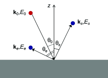
Figure 1: (Color online) Schematic drawing of the electron-induced electron-pair emission from surfaces.

We consider the process where, following the impact of a fast impinging electron with a momentum ${\bf k}_{0}$ and energy $E_{0}$, two electrons are emitted from the surface of a semiinfinite solid with momenta ${\bf k}_{s}$, ${\bf k}_{e}$ and energies $E_{s}$, $E_{e}$ (see Fig. 1). Hereafter the subscript $s~{}(e)$ stands for the scattered (ejected) electron. All the energies are measured with respect to the vacuum level, so that in vacuum we have the dispersion

$$k_{j}=\sqrt{2E_{j}}\qquad(j=0,s,e).$$

The rate of the discussed reaction is determined by the so-called (spin-averaged) fully differential cross section (FDCS) kouzakov02 ,

$$\frac{d\sigma}{dE_{s}d\Omega_{s}dE_{e}d\Omega_{e}} = \frac{k_{s}k_{e}}{(2\pi)^{5}k_{0}}\sum_{i_{\rm occ}}\left\{\frac{1}{4}|\langle{\bf k}_{s}{\bf k}_{e}|T|{\bf k}_{0}i\rangle+\langle{\bf k}_{e}{\bf k}_{s}|T|{\bf k}_{0}i\rangle|^{2}\right.$$ (1)

$$\left.+\frac{3}{4}|\langle{\bf k}_{s}{\bf k}_{e}|T|{\bf k}_{0}i\rangle-\langle{\bf k}_{e}{\bf k}_{s}|T|{\bf k}_{0}i\rangle|^{2}\right\}\delta(E_{s}+E_{e}-E_{0}-\epsilon_{i}).$$

Here we specified the directions of the momenta of the emitted electrons by the solid angles $\Omega_{s/e}$. The state vectors $|{\bf k}_{s}{\bf k}_{e}\rangle$ and $|{\bf k}_{0}i\rangle$ describe, respectively, the two final-state electrons with asymptotic momenta ${\bf k}_{s}$, ${\bf k}_{e}$ and the initial state consisting of the projectile state with momentum ${\bf k}_{0}$ and the valence-band state $|i\rangle$. The sum is taken over all occupied one-electron states of the surface with energy $\epsilon_{i}=E_{s}+E_{e}-E_{0}$. The operator $T$ is an effective transition operator that induces the $(e,2e)$ process and is assumed to be spin independent. In the frozen-core approximation it has the formal structure

$$T=V_{s}+W+(V_{s}+V_{e}+W)G^{+}_{se}(E_{tot})(V_{s}+W),$$ (2)

where $V_{s}$, $V_{e}$, and $W$ are effective (in general, optical) electron-solid and electron-electron potentials, respectively, and $G^{+}_{se}(E_{tot})$ is the retarded two-electron propagator in the potential $V_{s}+V_{e}+W$ at the total energy $E_{tot}=E_{s}+E_{e}$. The latter satisfies the Lippmann-Schwinger equation

$$G_{se}^{+}(E_{tot})=G_{0}^{+}(E_{tot})+G_{0}^{+}(E_{tot})(V_{s}+V_{e}+W)G_{se}^{+}(E_{tot}),$$ (3)

with $G_{0}^{+}(E_{tot})$ being the free two-electron propagator.

In what follows, we treat Eq. (2) only to the first order in the electron-electron interaction $W$. Such a procedure is usually justified by the choice of the kinematics such that $E_{0}\gg\Delta E$ $(\Delta E=E_{0}-E_{s})$ as well as by the screening of the electron-electron interaction due to the surrounding medium. This then amounts to the distorted wave Born approximation (DWBA)

$$T=\left[1+(V_{s}+V_{e})G^{+}_{s,e}(E_{tot})\right]W[1+G^{+}_{s,e}(E_{tot})V_{s}],$$ (4)

where $G^{+}_{s,e}(E_{tot})$ is the two-electron propagator in the potential $V_{s}+V_{e}$ and is given by the solution of the following Lippmann-Schwinger equation:

$$G_{s,e}^{+}(E_{tot})=G_{0}^{+}(E_{tot})+G_{0}^{+}(E_{tot})(V_{s}+V_{e})G_{s,e}^{+}(E_{tot}).$$ (5)

Taking into account Eq. (4), we can present FDCS (1) as

$$\frac{d\sigma}{d\epsilon_{s}d\Omega_{s}d\epsilon_{e}d\Omega_{e}} = \frac{k_{s}k_{e}}{(2\pi)^{5}k_{0}}\sum_{i_{\rm occ}}\left\{\frac{1}{4}|\langle\chi^{(-)}_{{\bf k}_{s}}\chi^{(-)}_{{\bf k}_{e}}|W|\chi^{(+)}_{{\bf k}_{0}}i\rangle+\langle\chi^{(-)}_{{\bf k}_{e}}\chi^{(-)}_{{\bf k}_{s}}|W|\chi^{(+)}_{{\bf k}_{0}}i\rangle|^{2}\right.$$ (6)

$$\left.+\frac{3}{4}|\langle\chi^{(-)}_{{\bf k}_{s}}\chi^{(-)}_{{\bf k}_{e}}|W|\chi^{(+)}_{{\bf k}_{0}}i\rangle-\langle\chi^{(-)}_{{\bf k}_{e}}\chi^{(-)}_{{\bf k}_{s}}|W|\chi^{(+)}_{{\bf k}_{0}}i\rangle|^{2}\right\}$$

$$\times\delta(E_{s}+E_{e}-E_{0}-\epsilon_{i}),$$

where

$$\chi^{(+)}_{{\bf k}_{0}}({\bf r}) = e^{i{\bf k}_{0}{\bf r}}+\int d{\bf r}^{\prime}e^{i{\bf k}_{0}{\bf r}^{\prime}}\upsilon({\bf r^{\prime}})g^{+}({\bf r^{\prime}},{\bf r};E_{0}),$$ (7)

$$\chi^{(-)}_{{\bf k}_{j}}({\bf r}) = e^{i{\bf k}_{j}{\bf r}}+\int d{\bf r}^{\prime}e^{i{\bf k}_{j}{\bf r}^{\prime}}\upsilon({\bf r^{\prime}})g^{-}({\bf r^{\prime}},{\bf r};E_{j}),$$ (8)

with $j=s,e$ and $V_{j}\equiv\upsilon$, and $g^{+}$ ($g^{-}$) being the retarded (advanced) one-electron Green’s function in the potential $\upsilon$. In the case of solids with a translational symmetry parallel to the surface, the states $\chi^{(\pm)}_{{\bf k}}$ can be calculated within the dynamical low-energy electron diffraction (LEED) theory leed ; luders01 .

Employing the surface dielectric function $\varepsilon$ for the description of the effect of the screening on the bare electron-electron interaction $\upsilon_{ee}$, we get

$$W({\bf r},{\bf r}^{\prime};\omega)=\int\,d{\bf r}^{\prime\prime}\varepsilon^{-1}({\bf r},{\bf r}^{\prime\prime};\omega)\upsilon_{ee}({\bf r}^{\prime\prime},{\bf r}^{\prime}),\qquad\upsilon_{ee}({\bf r}^{\prime\prime},{\bf r}^{\prime})=\frac{1}{|{\bf r}^{\prime\prime}-{\bf r}^{\prime}|},$$ (9)

where $\varepsilon^{-1}$ is the inverse dielectric function, and the energy argument $\omega$ ($\omega=E_{0}-E_{s}$ or $\omega=E_{0}-E_{e}$, depending on the final state of the incident electron) accounts for the dynamical screening effects.

III Surface dielectric response

For our purposes we need the inverse dielectric function $\varepsilon^{-1}$ that is derived from the dielectric function $\varepsilon$ according to

$$\int d{\bf r}^{\prime\prime}\varepsilon({\bf r},{\bf r}^{\prime\prime};\omega)\varepsilon^{-1}({\bf r}^{\prime\prime},{\bf r}^{\prime};\omega)=\int d{\bf r}^{\prime\prime}\varepsilon^{-1}({\bf r},{\bf r}^{\prime\prime};\omega)\varepsilon({\bf r}^{\prime\prime},{\bf r}^{\prime};\omega)=\delta({\bf r}-{\bf r}^{\prime}).$$ (10)

Let us assume that the $z$ axis is perpendicular to the surface and that the solid sample fills the $z<0$ region (see Fig. 1). If the sample is crystalline, then

$$\varepsilon({\bf r},{\bf r}^{\prime};\omega)=\varepsilon({\bf r}+{\bf A},{\bf r}^{\prime}+{\bf A};\omega),\qquad\varepsilon^{-1}({\bf r},{\bf r}^{\prime};\omega)=\varepsilon^{-1}({\bf r}+{\bf A},{\bf r}^{\prime}+{\bf A};\omega),$$ (11)

where ${\bf A}$ is the lattice vector parallel to the surface. Thus, $\varepsilon$ and $\varepsilon^{-1}$ can be presented as

$$\varepsilon({\bf r},{\bf r}^{\prime};\omega) = \sum_{{\bf G},{\bf G}^{\prime}}e^{i({\bf G}{\bf R}-{\bf G}^{\prime}{\bf R}^{\prime})}\int\limits_{\rm 1^{st}\,BZ}\frac{d{\bf Q}}{(2\pi)^{2}}\,\varepsilon_{{\bf G},{\bf G}^{\prime}}({\bf Q},z,z^{\prime};\omega)e^{i{\bf Q}({\bf R}-{\bf R}^{\prime})},$$ (12)

$$\varepsilon^{-1}({\bf r},{\bf r}^{\prime};\omega) = \sum_{{\bf G},{\bf G}^{\prime}}e^{i({\bf G}{\bf R}-{\bf G}^{\prime}{\bf R}^{\prime})}\int\limits_{\rm 1^{st}\,BZ}\frac{d{\bf Q}}{(2\pi)^{2}}\,\varepsilon_{{\bf G},{\bf G}^{\prime}}^{-1}({\bf Q},z,z^{\prime};\omega)e^{i{\bf Q}({\bf R}-{\bf R}^{\prime})},$$ (13)

where ${\bf r}=({\bf R},z)$ and ${\bf r}^{\prime}=({\bf R}^{\prime},z^{\prime})$, ${\bf G}$ and ${\bf G}^{\prime}$ are the surface reciprocal lattice vectors, and the ${\bf Q}$ integration is carried over the first Brillouin zone ($1^{\rm st}$ BZ) of the surface reciprocal lattice. Using Eq. (13), we get for the screened Coulomb potential (9)

$$W({\bf r},{\bf r}_{0};\omega) = \sum_{{\bf G},{\bf G}^{\prime}}e^{i({\bf G}{\bf R}-{\bf G}^{\prime}{\bf R}_{0})}\int\limits_{\rm 1^{st}\,BZ}\frac{d{\bf Q}}{2\pi}\,\frac{e^{i{\bf Q}({\bf R}-{\bf R}_{0})}}{|{\bf Q}+{\bf G}^{\prime}|}\int dz^{\prime}\varepsilon_{{\bf G},{\bf G}^{\prime}}^{-1}({\bf Q},z,z^{\prime};\omega)e^{-|{\bf Q}+{\bf G}^{\prime}||z^{\prime}-z_{0}|}.$$

If we neglect the crystalline effects on $\varepsilon$ and $\varepsilon^{-1}$ parallel to the surface, then

$$\varepsilon^{-1}_{{\bf G},{\bf G}^{\prime}}({\bf Q},z,z^{\prime};\omega)=\delta_{{\bf G},{\bf G}^{\prime}}\varepsilon^{-1}({\bf Q}+{\bf G},z,z^{\prime};\omega),$$ (15)

where it is assumed that ${\bf Q}\in 1^{\rm st}$ BZ, and hence

$$W({\bf r},{\bf r}_{0};\omega)=\int\frac{d{\bf Q}}{2\pi}\,\frac{e^{i{\bf Q}({\bf R}-{\bf R}_{0})}}{Q}\int dz^{\prime}\varepsilon^{-1}({\bf Q},z,z^{\prime};\omega)e^{-Q|z^{\prime}-z_{0}|}.$$ (16)

Representations (III) and (16) can be particularly useful, when employing the following expansion of the electron states in Eq. (6):

$$\chi^{(\pm)}_{\bf k}({\bf r})=\sum_{\bf G}C_{\bf k}^{(\pm)}({\bf G},z)e^{i({\bf K}+{\bf G}){\bf R}},$$ (17)

where ${\bf k}=({\bf K},k_{z})$.

If the sample is a free-electron metal (for instance, Al or Be), then the model of a degenerate electron gas where electrons move in a positive ionic background and are bounded by a surface potential barrier is commonly applicable to mimic its dielectric properties. Below, we briefly sketch two possible approaches for describing the dielectric response of such jellium-like systems.

III.1 Specular-reflection model

The problems involving the interaction of charged particles with plane-bounded solids are often treated using SRM. This model assumes the surface barrier to be impermeable for the electrons in the solid, so that they are specularly reflected at the surface. The reflection process is described in a classical fashion, in particular the interference between the incoming and outgoing components is neglected. Within SRM the potential created by the external charge distribution $\rho({\bf r},t)$ in the vicinity of a surface is given by (see, for instance, Ref. echenique92 and references therein)

$$V({\bf r},t)=V_{+}({\bf r},t)\Theta(z)+V_{-}({\bf r},t)\Theta(-z),\qquad V_{\pm}({\bf r},t)=\int\frac{d{\bf Q}}{(2\pi)^{2}}\int\frac{d\omega}{2\pi}\,V_{\pm}({\bf Q},z;\omega)e^{i({\bf QR}-\omega t)},$$ (18)

where

$$V_{\pm}({\bf Q},z;\omega)=4\pi[U_{\pm}({\bf Q},z;\omega)\mp\tilde{\rho}({\bf Q},\omega)\nu_{\pm}({\bf Q},z;\omega)],$$ (19)

with [using the notation ${\bf q}=({\bf Q},q_{z})$]

$$U_{+}({\bf Q},z;\omega)=\int\frac{dq_{z}}{2\pi}\frac{\rho_{+}({\bf q},\omega)}{q^{2}}\,e^{iq_{z}z},\qquad U_{-}({\bf Q},z;\omega)=\int\frac{dq_{z}}{2\pi}\frac{\rho_{-}({\bf q},\omega)}{q^{2}\varepsilon_{b}({\bf q},\omega)}\,e^{iq_{z}z},$$ (20)

$$\rho_{\pm}({\bf q},\omega)=\int d{\bf r}\int dt\,\rho({\bf R},\pm|z|,t)e^{-i({\bf qr}-\omega t)},$$

$$\nu_{+}({\bf Q},z;\omega)=\int\frac{dq_{z}}{2\pi}\frac{2Q}{q^{2}}\,e^{iq_{z}z}=e^{-Q|z|},\qquad\nu_{-}({\bf Q},z;\omega)=\int\frac{dq_{z}}{2\pi}\frac{2Q}{q^{2}\varepsilon_{b}({\bf q},\omega)}\,e^{iq_{z}z},$$ (21)

$$\tilde{\rho}({\bf Q},\omega)=\frac{1}{1+\varepsilon_{s}({\bf Q},\omega)}[U_{+}({\bf Q},0;\omega)-U_{-}({\bf Q},0;\omega)],\qquad\varepsilon_{s}({\bf Q},\omega)=\nu_{-}({\bf Q},0;\omega).$$ (22)

In Eqs. (20) and (21), $\varepsilon_{b}({\bf q},\omega)$ is the bulk dielectric function, i.e., that of an infinite 3D system. The quantity $\varepsilon_{s}({\bf Q},\omega)$ occurring in Eq. (22) is the so-called surface dielectric function newns70 .

To utilize the SRM approach in the present quantum-mechanical treatment, the external charge density $\rho({\bf r},t)$ must be replaced by the corresponding operator $\rho({\bf r},t)=e^{-iH_{0}t}\rho({\bf r})e^{iH_{0}t}$, where $H_{0}$ is the Hamiltonian associated with the incident electron. Clearly, in this way the frequency $\omega$ equals the energy transfer $\Delta E=E_{0}-E_{s(e)}$. Since $\rho({\bf r})=\delta({\bf r}-{\bf r}_{0})$, where ${\bf r}_{0}$ is the position of the incident electron, it is straightforward to show that the resulting expression for the inverse dielectric function in Eq. (16) is

$$\varepsilon^{-1}({\bf Q},z,z^{\prime};\omega) = \Theta(z)\left\{\delta(z-|z^{\prime}|)\Theta(z_{0})-\frac{2e^{-Qz}}{1+\varepsilon_{s}({\bf Q},\omega)}[\delta(z^{\prime})\Theta(z_{0})-\kappa({\bf Q},z^{\prime};\omega)\Theta(-z_{0})]\right\}$$ (23)

$$+\Theta(-z)\Bigg{\{}[\kappa({\bf Q},z+z^{\prime};\omega)+\kappa({\bf Q},z-z^{\prime};\omega)]\Theta(-z_{0})+\frac{2\nu_{-}({\bf Q},z;\omega)}{1+\varepsilon_{s}({\bf Q},\omega)}$$

$$\times[\delta(z^{\prime})\Theta(z_{0})-\kappa({\bf Q},z^{\prime};\omega)\Theta(-z_{0})]\Bigg{\}},$$

where

$$\kappa({\bf Q},z;\omega)=\int\limits^{\infty}_{-\infty}\frac{dq_{z}}{2\pi}\frac{e^{iq_{z}z}}{\varepsilon_{b}({\bf q},\omega)}.$$ (24)

Note that the inverse dielectric function (23) depends on whether the incoming electron is inside ($z_{0}<0$) or outside ($z_{0}>0$) the solid.

III.2 Random phase approximation

RPA constitutes a reasonable framework for describing the dielectric response of a degenerate electron gas. The bulk dielectric function $\varepsilon_{b}$ was first derived within this method by Lindhard lindhard . For the case of a semi-infinite geometry a very useful study is from Newns newns70 , who considered the dielectric response of a semi-infinite ideal metal within RPA assuming an infinite surface barrier (RPA-IB), which is in the spirit of SRM. Using the approximation of a specular electron reflection, Bechstedt et al. bechstedt83 derived expressions for the screened Coulomb potential and the inverse dielectric function. However, Horing et al. horring85 noticed that the result of Ref. bechstedt83 is incapable of describing correctly the image field as a part of the dynamically screened Coulomb potential. In their calculation, Horing et al. utilized the potential solutions obtained by Newns newns70 within the RPA-IB model. Employing the mathematical model delta-function potential as a bare, unscreened interaction and neglecting the nondiagonal elements in the density-response matrix, they calculated the inverse dielectric function as

$$\varepsilon^{-1}({\bf Q},z,z^{\prime};\omega) = \Theta(z)\left\{\delta(z-z^{\prime})-\frac{e^{-Qz}}{1+\varepsilon_{s}({\bf Q},\omega)}[\delta(z^{\prime})-2\kappa({\bf Q},z^{\prime};\omega)\Theta(-z^{\prime})]\right\}$$ (25)

$$+\Theta(-z)\Bigg{\{}[\kappa({\bf Q},z+z^{\prime};\omega)+\kappa({\bf Q},z-z^{\prime};\omega)]\Theta(-z^{\prime})+\frac{\nu_{-}({\bf Q},z;\omega)}{1+\varepsilon_{s}({\bf Q},\omega)}$$

$$\times[\delta(z^{\prime})-2\kappa({\bf Q},z^{\prime};\omega)\Theta(-z^{\prime})]\Bigg{\}},$$

where the functions $\kappa({\bf Q},z;\omega)$, $\nu_{-}({\bf Q},z;\omega)$, and $\varepsilon_{s}({\bf Q},\omega)$ are the same as in Sec. III.1.

Expressions (23) and (25) have a similar structure. Moreover, one can formally deduce Eq. (25) using the SRM approach in the case of the model delta-function potential $\upsilon_{ee}({\bf r},{\bf r}_{0})=\delta({\bf r}-{\bf r}_{0})$. However, the RPA-IB result (25) is supposed to be applicable in the case of Coulomb-like potentials as well (see Ref. horring85 for detail). The latter feature makes the two approaches nonequivalent.

IV Results and discussion

In this section we present and analyze the numerical results for the correlated electron-pair emission from Al and Be surfaces. To be specific, we consider the kinematics of the recent experimental study on Al werner08 . In that experiment, the electron energy loss was measured at the incident energy $E_{0}=100$ eV and the angle $\theta_{0}=30^{\circ}$ in the specular reflection mode, that is, $\theta_{s}=30^{\circ}$, in coincidence with the secondary electron ejected at the angle $\theta_{e}=60^{\circ}$ (see Fig. 1). We neglect the crystalline effects in our calculations and construct the one-electron states in Eq. (6) in the context of the jellium model. The details of this procedure are given in the Appendix. The surface dielectric response is taken into account within the SRM and RPA-IB approaches described in the previous section. Each of them depends on the model of the bulk dielectric response. Below we outline two approximations for the bulk dielectric function of a free-electron metal that were employed in the present calculations: (i) the Thomas-Fermi (TF) ashcroft_book and (ii) the hydrodynamic (HA) bloch33 approximations. In spite of their relative simplicity, they efficiently mimic the basic features pertinent to the static and dynamical bulk screening effects in metals. In addition, their use in the calculations makes the numerical implementation more transparent and controllable.

IV.0.1 Thomas-Fermi approximation

This well-known model neglects the dynamical screening effects and assumes the dielectric function to be of the form

$$\varepsilon_{b}(q,\omega)=1+\frac{\lambda^{2}}{q^{2}},$$ (26)

where $\lambda$ is the screening constant. For a free-electron isotropic gas one has

$$\lambda^{2}=\frac{4k_{F}}{\pi},\qquad k_{F}=\sqrt{2\epsilon_{F}},$$

where $\epsilon_{F}$ and $k_{F}$ are the Fermi energy and momentum, respectively. Using the Wigner-Seitz radius $r_{s}$, we have

$$\lambda^{2}=\left(\frac{12}{\pi}\right)^{2/3}\frac{1}{r_{s}}$$

($r_{s}=2.07$ for Al and $r_{s}=1.87$ for Be).

Within the TF model the functions in Eqs. (23) and (25) are given by

$$\kappa({\bf Q},z;\omega)=\delta(z)-\frac{\lambda^{2}}{2\Lambda}\,e^{-\Lambda|z|},\qquad\nu_{-}({\bf Q},z;\omega)=\frac{Q}{\Lambda}\,e^{-\Lambda|z|},\qquad\varepsilon_{s}({\bf Q},\omega)=\frac{Q}{\Lambda},$$ (27)

where $\Lambda=\sqrt{Q^{2}+\lambda^{2}}$.

IV.0.2 Hydrodynamic approximation

Since its introduction almost 80 years ago bloch33 , the hydrodynamic approximation has proved to be very useful in describing the electrical transport and the optical properties of conductors. The main advantage of this model lies in the simplicity of accounting for the spatial dispersion,

$$\varepsilon_{b}(q,\omega)=1+\frac{\omega_{b}^{2}}{\beta^{2}q^{2}-\omega(\omega+i\nu)},$$ (28)

where the frequency of the bulk plasmon mode $\omega_{b}$ is given by

$$\omega_{b}=\sqrt{4\pi n}=\sqrt{\frac{3}{r_{s}^{3}}},$$

with $n$ being the electron density. The parameter $\beta$ depends on $\omega$, such that

$$\beta=\left\{\begin{array}[]{l}\displaystyle\sqrt{\frac{1}{3}}\upsilon_{F},\qquad\omega\ll\nu\\ \displaystyle\sqrt{\frac{3}{5}}\upsilon_{F},\qquad\omega\gg\nu.\end{array}\right.$$ (29)

The above low- and high-frequency limits can be reproduced with the “interpolation formula” halevi95

$$\beta^{2}=\frac{\frac{3}{5}\omega+\frac{1}{3}i\nu}{\omega+i\nu}\upsilon_{F}^{2}.$$ (30)

The collision frequency $\nu$ can be estimated as $\nu\sim\Gamma_{pl}$ ($\Gamma_{pl}=0.53$ eV for Al and $\Gamma_{pl}=4.7$ eV for Be). Note that the TF result (26) derives from Eq. (28) in the limit $\omega\to 0$.

Within the HA model the functions in Eqs. (23) and (25) are given by

$$\kappa({\bf Q},z;\omega) = \delta(z)-\frac{\omega_{b}^{2}}{2\beta^{2}}\,\frac{e^{-\Lambda|z|}}{\Lambda},$$

$$\qquad\nu_{-}({\bf Q},z;\omega) = \frac{\omega(\omega+i\nu)e^{-Q|z|}}{\omega(\omega+i\nu)-\omega_{b}^{2}}-\frac{Q}{\Lambda}\,\frac{\omega_{b}^{2}e^{-\Lambda|z|}}{\omega(\omega+i\nu)-\omega_{b}^{2}},$$

$$\qquad\varepsilon_{s}({\bf Q},\omega) = \frac{\omega(\omega+i\nu)\Lambda-\omega_{b}^{2}Q}{[\omega(\omega+i\nu)-\omega_{b}^{2}]\Lambda},$$ (31)

where $\Lambda=-i\beta^{-1}\sqrt{\omega(\omega+i\nu)-\omega_{b}^{2}-\beta^{2}Q^{2}}$ (here the first branch of the square root function is assumed, which yields ${\rm Re}(\Lambda)>0$).

IV.1 Aluminum

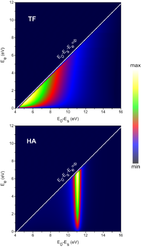
Figure 2: (Color online) Correlated electron energy distribution from Al within SRM. The top panel corresponds to the TF bulk dielectric function, while the bottom corresponds to HA. The white solid line marks the energy threshold for the electron-pair emission, $E_{0}-E_{s}-E_{e}\geq\Phi$, where $\Phi$ is the work function.

Fig. 2 shows the correlated electron energy distribution of the scattered and the ejected electrons calculated using the SRM surface dielectric function (23). Marked differences between the TF and HA models can be seen. The maximum of the intensity in the TF case is located at small values of $E_{e}\sim 1$ eV when the energy loss $\Delta E=E_{0}-E_{s}$ exceeds the work function $\Phi=4.3$ eV by approximately the same amount, which indicates that the ejected electron originates from the initial state close to the Fermi level $\epsilon_{F}$. With increasing $\Delta E$ the intensity decreases and a tendency can be observed: at a given energy-loss value the electrons are preferably ejected with energies close to the threshold $E_{e}=\Delta E-\Phi$, which corresponds to $\epsilon_{i}=\epsilon_{F}$. The latter is readily explained by the fact that the density of states at the Fermi level is maximal. In contrast to the TF model, in the HA case the intensity is strongly peaked around $\Delta E\approx 11$ eV which is slightly above the surface plasmon energy $\omega_{s}=\omega_{b}/\sqrt{2}=10.5$ eV. The reason for such a resonant behavior is due to the poles of the function $(\ref{srm})$ when $1+\varepsilon_{s}=0$. If neglecting the plasmon dispersion and the damping effects in the HA model (28), that is, $\beta=0$ and $\nu=0$, one finds that, according to Eq. (IV.0.2), the pole is located exactly at $\Delta E=\omega_{s}$. The plasmon dispersion and the damping effects are responsible for the shift and for the finite width of the observed resonant peak.

The numerical results for the correlated electron energy distribution using the RPA-IB surface dielectric function (25) are presented in Fig. 3. The TF distribution is very close to that when using SRM. However, in the HA case the distribution differs from the analogous one in Fig. 2. Namely, in addition to the peak associated with the surface plasmon there appears another, more pronounced feature at approximately $\Delta E=15$ eV. Taking into account that $\omega_{b}=14.9$ eV, it is clear that the feature is due to the dynamical screening effects related to the bulk-plasmon mode. The absence of the bulk-plasmon peak in the SRM case and its appearance in the RPA-IB case follows from the comparison of Eqs. (23) and (25). The bulk screening effects in these models are associated with function (24). Thus, within the SRM (23) it comes into play when the incident electron penetrates inside the metal ($z_{0}<0$), while within the RPA-IB (25) it becomes already relevant when the incident electron is still moving in the vacuum. A short inelastic mean free path for the incoming electron results in small penetration lengths, thus strongly restricting the bulk contribution in the SRM case.

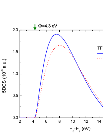
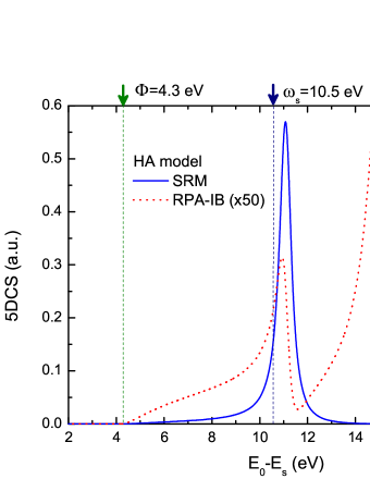
Figure 4: (Color online) Dependence of the ejected-electron yields from Al on the energy loss within SRM and RPA-IB. The top (bottom) panel presents the results using the TF (HA) bulk dielectric function.

Fig. 4 compares the so-called five-fold differential cross sections (5DCS), which derive from FDCS (6) upon integrating over the ejected electron energy $E_{e}$, using the SRM and RPA-IB approaches. Clearly, 5DCS characterizes the dependence of the ejected-electron yield on the energy loss $\Delta E$ in the considered collision geometry. In accordance with the TF results in Figs. 2 and 3, the TF ejected-electron yields in Fig. 4 are very close to each other, starting to grow at the threshold value $\Delta E=\Phi$, exhibiting maximum at $\Delta E=7-8$ eV, and then smoothly decreasing down to 0 at $\Delta E\approx 16$ eV, which is due to the restriction $|{\bf K}_{s}+{\bf K}_{e}-{\bf K}_{0}|\leq k_{F}$ imposed by the conservation of the electron-pair momentum parallel to the surface. The HA results are orders of magnitude larger than the TF ones, indicating the strength of the dynamical screening effects. In accordance with Figs. 2 and 3, the HA results in Fig. 4 using SRM exhibit only one peak associated with the surface-plasmon mode while those using RPA-IB two peaks which are due to both the surface- and the bulk-plasmon modes. The intensity of the surface-plasmon peak in the SRM case exceeds that in the RPA-IB case by almost two orders of magnitude. The position and the intensity of the bulk-plasmon peak in the RPA-IB case is mainly determined by the interplay between the plasmon pole in the HA bulk dielectric function and the kinematical effects related to the conservation of the electron-pair energy and the surface-parallel momentum.

IV.2 Beryllium

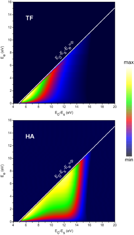
Figure 5: (Color online) The same as in Fig. 2, but in the case of Be.

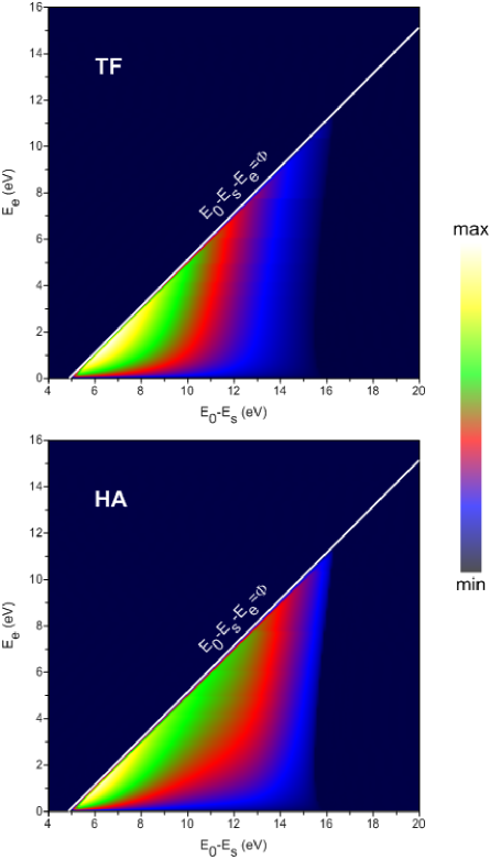
Figure 6: (Color online) The same as in Fig. 3, but in the case of Be.

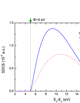
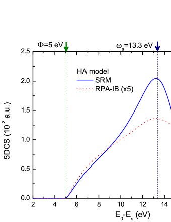
Figure 7: (Color online) The same as in Fig. 4, but in the case of Be.

Figs. 5, 6, and 7 present numerical calculations for the same situations as in Figs. 2, 3, and 4, respectively, but for Be. In the HA case, the differences compared to the results for Al can be attributed to a much wider plasmon resonance in Be. In particular, we find that the footprints of the plasmon modes in the HA results are much weaker and broader. The role of the plasmon linewidth $\Gamma_{pl}$ is clearly seen when comparing the HA results for Al and Be using SRM. The FWHM of the peaks observed in the HA results within SRM in Figs. 4 and 7 are given by approximately $\Gamma_{pl}({\rm Al})=0.53$ eV and $\Gamma_{pl}({\rm Be})=4.7$ eV, respectively. Moreover, when using RPA-IB, the plasmon features can hardly be identified in FDCS (Fig. 6). And they manifest themselves for some cases only in 5DCS (Fig. 7). In contrast, the TF results for Be are rather close to those for Al, particularly in magnitude. Though the differences between the TF and HA results in Figs. 5 and 6 are not as large as in the case of Al, the effects of dynamical screening are still quite strong. This conclusion follows from the fact that the HA results for 5DCS are about four orders of magnitude lager than the TF ones (see Fig. 7).

V Theory and experiment

Here we discuss how the predictions of the present theoretical approach compare to the results of the recent experiments on Al werner08 ; werner11 . The kinematical regime of Ref. werner08 was specified in the previous section. The measurements in Ref. werner11 were carried out for a normal incidence ($\theta_{0}=0^{\circ}$) of the projectile electron with an impact energy of 500 eV. The scattered and the ejected electrons were detected at the polar angles $\theta_{s}=\theta_{e}=60^{\circ}$ (see Fig. 1). In both studies, the secondary-electron spectra were recorded in coincidence with the primary electron having undergone an energy loss that is equal to the bulk- or the surface-plasmon frequencies, i.e., when $\Delta E=\omega_{b}$ and $\Delta E=\omega_{s}$. In coincident measurements of the secondary-electron spectra in Ref. werner11 , further data were reported for the energy-loss values of 25, 30, 40, 45, and 150 eV.

For a detailed quantitative comparison of our theoretical results with the discussed measurements one should consider the following aspects. First, the experimental data are reported on an arbitrary intensity scale, which means that the absolute values of the FDCS are not determined. Second, one must bear in mind that the experimental data are broadened by a finite energy and angular resolution whose effective values in Ref. werner08 were given to be 1 and 1.2 eV for the primary (scattered) and the secondary (ejected) electrons, respectively, while in Ref. werner11 the overall energy resolution was reported to be about 5 eV. Below we take into account the energy-broadening effect by convoluting our theoretical calculations with a Gaussian energy distribution.

Figs. 8 and 9 show the results of the numerical calculations for the FDCS in the kinematics of Ref. werner08 , which were convoluted with the 2D Gaussian function

$$P(E_{s}^{\prime},E_{e}^{\prime})=\frac{1}{2\pi\sigma_{s}\sigma_{e}}\exp\left[-\frac{(E_{s}^{\prime}-E_{s})^{2}}{2\sigma_{s}^{2}}-\frac{(E_{e}^{\prime}-E_{e})^{2}}{2\sigma_{e}^{2}}\right],\qquad\sigma_{s(e)}=\frac{{\rm FWHM}_{s(e)}}{2\sqrt{2\ln 2}},$$ (32)

where ${\rm FWHM}_{s}=1$ eV and ${\rm FWHM}_{e}=1.2$ eV. As remarked above, the absolute values were not measured in the experiment, but the scale for the two coincidence spectra (at $\Delta E=\omega_{b}$ and $\Delta E=\omega_{s}$) in Ref. werner08 is the same. In order to place the experimental results on a common intensity scale with the theory in each panel of Figs. 8 and 9, they are normalized in such a way that the maximal experimental and theoretical values of the FDCS corresponding to the $\Delta E=\omega_{s}$ case are the same. In terms of the positions of the peaks in the secondary-electron spectra, all calculations agree reasonably well with experiments. However, in contrast to the experimental results, the theoretical spectra exhibit appreciable intensities in the region $E_{e}\lesssim 4$ eV. With regard to a comparison of the intensities in the $\Delta E=\omega_{b}$ and $\Delta E=\omega_{s}$ cases, only the RPA-IB model using the HA bulk dielectric function provides a reasonable agreement with experiment. Indeed, the TF approximation, both within RPA-IB and within SRM, predicts the $\Delta E=\omega_{s}$ results that are by an order of magnitude larger than the $\Delta E=\omega_{b}$ ones, while the SRM model using HA yields an even much larger discrepancy (almost three orders of magnitude). Thus, it can be concluded that within the present theoretical approach the best overall agreement with the experimental data of Ref. werner08 is found when using the RPA-IB model that involves the HA bulk dielectric function. This comparison hints at the suitability of the measurements to asses the reliability of the employed dielectric response. We note, however, that further comparisons with measurements at different geometries, as well as on different samples, are necessary for conclusive statements on the quality of the discussed approximations.

The experimental conditions chosen in Ref. werner11 are beyond the validity range and the initial scope of our theoretical treatment. In fact, in this case the theoretical FDCS vanishes for all $\Delta E$ that were chosen in the experiment. The reason for this is that in the theory we do not account for coherent or incoherent multi-scattering events that randomize the momenta. As a result we are bound to the kinematical limitation $|{\bf K}_{s}+{\bf K}_{e}-{\bf K}_{0}|\leq k_{F}$ that stems from the assumption of an electron ejection upon a direct electron-electron scattering. In principle, one may lift this limitation within the present theoretical approach by taking into account the effects of electron-pair diffraction diffPRL ; samarin04 and surface roughness. In our opinion this would be, however, insufficient to explain the dominant, broad peak-like structures with a falling edge at about $E_{e}=\omega_{b}-\Phi$ that are observed in the measured coincidence spectra when $\Delta E$ exceeds largely the $\omega_{b}$ value. Clearly, due to the energy balance, these features can not be accounted for within the picture of only one inelastic electron-electron collision involving either plasmon decay or dynamical screening effects. The experimental findings werner11 thus hint at the existence of multiple inelastic scattering in the kinematics under study. In this context we remark that the influence of these multiple-scattering processes on the pair correlation functions was discussed and experimentally verified for a LiF sample in Ref. schumann05 . In Ref. werner11 it was argued that multiple-scattering processes can be viewed as a Markov chain, with independent successive inelastic collisions leading to the excitation of the surface and the bulk plasmons followed by their decay into single electron-hole pairs (see Ref. werner11 for detail). We add that one cannot rule out the scenario in which the individual inelastic events in the Markov chain take place due to direct electron-electron scattering resonantly enhanced at the energy transfers close to the surface- and the bulk-plasmon frequencies.

VI Summary and conclusions

In summary, we considered theoretically the electron energy-loss process accompanied by the ejection of the secondary electron from a clean metallic surface. Our study was focused on the effects of the surface dielectric properties in the discussed process. Restricting the analysis by the mechanism of a direct electron-electron scattering, we took into account the modification of the bare Coulomb potential due to the surrounding medium by means of the inverse dielectric function. Using two models of the inverse dielectric function of the surface, SRM and RPA-IB, we performed numerical calculations for Al and Be with and without accounting for the dynamical screening. We found that the results exhibit clear plasmon features in the case of Al, while in the case of Be these features are much less pronounced, which can be attributed to a wider plasmon resonance in Be. For both metals, very strong dynamical-screening effects were found.

In the present theoretical analysis we did not address the issue of the plasmon-decay mechanism which also contributes to the considered process. Studying this specific mechanism with the $(e,2e)$ method can offer an opportunity for the detailed investigation of the plasmon-decay channel into a single electron-hole pair. For instance, the recent experimental results from Al werner08 showed clear surface- and bulk-plasmon features in FDCS that were interpreted in Ref. werner08 within the plasmon-decay model. However, as shown by our RPA-IB HA calculations in Fig. 8, these features can be interpreted within the direct-scattering model as well. As stated in the Introduction the role of the plasmon-decay mechanism is expected to be more significant in free-electron-type metals exhibiting a broad plasmon resonance, such as Be. However, to our knowledge, no coincidence $(e,2e)$ measurements on such materials have been published so far.

Thus, further experimental studies on the plasmon-assisted $(e,2e)$ collisions at metallic surfaces are desirable in order to shed more light on the roles of the discussed mechanisms. On the other hand, to account for experimental observation theory must go beyond the framework of a single inelastic collision.

Appendix A One-electron states

Evaluation of the FDCS (6) requires the knowledge of the one-electron states that correspond to the incoming (incident), bound, and outgoing (scattered and ejected) electrons. Let us consider a semiinfinite metallic sample filling the space in the negative $z$ direction. Within the jellium model, the effective one-electron potential $V$ is a steplike one, i.e.,

$$V=-V_{0}\Theta(-z).$$ (33)

For a clean metallic material one has

$$V_{0}=\epsilon_{F}+\Phi,$$ (34)

where $\Phi$ is the work function. The wave function and the energy of the electron bound in the metal are thus given by

$$\chi_{\bf k}({\bf r})=e^{i{\bf KR}}\left\{B(k_{z})e^{-\gamma z}\Theta(z)+[e^{ik_{z}z}+A(k_{z})e^{-ik_{z}z}]\Theta(-z)\right\},\qquad\epsilon_{\bf k}=\frac{1}{2}({\bf K}^{2}+k_{z}^{2})-V_{0},$$ (35)

where

$$A(k_{z})=\frac{k_{z}-i\gamma}{k_{z}+i\gamma},\qquad B(k_{z})=\frac{2k_{z}}{k_{z}+i\gamma},\qquad\gamma=\sqrt{2V_{0}-k_{z}^{2}},$$ (36)

and $\sqrt{2V_{0}}\geq k_{z}\geq 0$.

Within the SRM and RPA-IB approaches the surface barrier is impermeable for electrons in the metal. This feature can be taken into account by calculating the wave function in Eq. (35) under the assumption $V_{0}=\infty$, which yields

$$\chi_{\bf k}({\bf r})=2e^{i{\bf KR}}\sin(k_{z}z)\Theta(-z).$$ (37)

The incoming and the outgoing electron states with momentum ${\bf k}=({\bf K},k_{z})$ and the energy $E_{\bf k}=({\bf K}^{2}+k_{z}^{2})/2$ in the potential (33) are given by

$$\chi^{(+)}_{\bf k}({\bf r}) = e^{i{\bf KR}}\left\{[e^{ik_{z}z}+R(k_{z})e^{-ik_{z}z}]\Theta(z)+D(k_{z})e^{ik_{z}^{\prime}z}e^{\alpha z}\Theta(-z)\right\}\qquad(k_{z}<0),$$ (38)

$$\chi^{(-)}_{\bf k}({\bf r}) = e^{i{\bf KR}}\left\{e^{ik_{z}z}\Theta(z)+[A_{1}(k_{z})e^{ik_{z}^{\prime}z}+A_{2}(k_{z})e^{-ik_{z}^{\prime}z}]e^{\alpha z}\Theta(-z)\right\}\qquad(k_{z}>0),$$ (39)

where

$$R(k_{z})=\frac{k_{z}-k_{z}^{\prime}+i\alpha}{k_{z}+k_{z}^{\prime}-i\alpha},\qquad D(k_{z})=\frac{2k_{z}}{k_{z}+k_{z}^{\prime}-i\alpha},$$

$$A_{1}(k_{z})=\frac{k_{z}^{\prime}+k_{z}+i\alpha}{2k_{z}^{\prime}},\qquad A_{2}(k_{z})=\frac{k_{z}^{\prime}-k_{z}-i\alpha}{2k_{z}^{\prime}},$$

$$k_{z}^{\prime}=\mbox{sgn}(k_{z})\sqrt{\frac{k_{z}^{2}+2V_{0}+[(k_{z}^{2}+2V_{0})^{2}+4V_{0i}^{2}]^{1/2}}{2}},\qquad\alpha=\frac{V_{0i}}{|k_{z}^{\prime}|},$$

with $V_{0i}$ being introduced as an imaginary component of the potential,

$$V=(-V_{0}+iV_{0i})\Theta(-z),$$

to mimic the damping of the electron waves inside the metal. Using the concept of the inelastic mean free path $\lambda$, it can be estimated as

$$V_{0i}=\frac{k^{\prime}}{2\lambda},\qquad k^{\prime}=\sqrt{2(E_{\bf k}+V_{0})}.$$

One can calculate $\lambda$, for instance, from the parametrization formula by Seah and Dench seah79 , which in the case of the elemental materials reads

$$\lambda=\frac{538a}{(E_{\bf k}+\Phi)^{2}}+0.41\sqrt{a^{3}(E_{\bf k}+\Phi)},$$ (41)

where the electron energy $E_{\bf k}+\Phi$ is measured in eV. The average thickness of the monolayer $a$ measured in nanometers is given by

$$a^{3}=\frac{10^{24}M}{\rho N_{A}},$$ (42)

where $M$ is the atomic weight, $\rho$ is the bulk density (in kg/m³), and $N_{A}$ is Avogadro’s number.

Figure 3: (Color online) The same as in Fig. 2, but using RPA-IB.

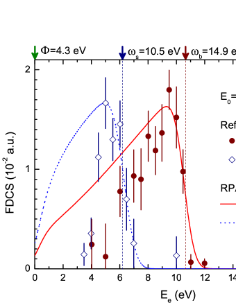
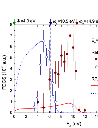
Figure 8: (Color online) Spectra of secondary electrons at energy losses equal to the surface- and bulk-plasmon frequencies. The calculations were carried out within the RPA-IB model using the HA (top panel) and TF (bottom panel) bulk dielectric functions. The experimental data points are borrowed from Ref. werner08 .

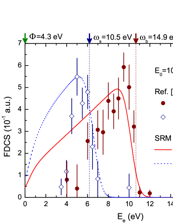
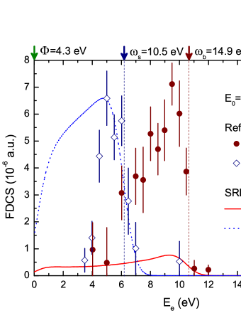
Figure 9: (Color online) The same as in Fig. 8, but within the SRM model.

References

- (1) R. Byrdson, Electron Energy Loss Spectrosocpy (BIOS Scientific, Oxford, 2001).
- (2) J. Kirschner, O. M. Artamonov, and S. N. Samarin, Phys. Rev. Lett. 75, 2424 (1995).
- (3) F. O. Schumann, J. Kirschner, and J. Berakdar, Phys. Rev. Lett. 95, 117601 (2005).
- (4) F. O. Schumann, C. Winkler, J. Kirschner, F. Giebels, H. Gollisch, and R. Feder, Phys. Rev. Lett. 104, 087602 (2010).
- (5) E. Weigold and I. E. McCarthy, Electron Momentum Spectroscopy (Kluwer, New York, 1999).
- (6) J. Berakdar, Phys. Rev. Lett. 83, 5150 (1999).
- (7) S. N. Samarin, J. Berakdar, O. Artamonov, and J. Kirschner, Phys. Rev. Lett. 85, 1746 (2000).
- (8) A. Morozov, J. Berakdar, S. N. Samarin, F. U. Hillebrecht, and J. Kirschner, Phys. Rev. B 65, 104425 (2002).
- (9) J. Berakdar, M. P. Das, Phys. Rev. A 56, 1403 (1997).
- (10) J. Berakdar, S. N. Samarin, R. Herrmann, and J. Kirschner, Phys. Rev. Lett. 81, 3535 (1998).
- (11) H. Gollisch, T. Scheunemann, and R. Feder, Solid State Commun. 117, 691 (2001).
- (12) J. Berakdar, H. Gollisch, and R. Feder, Solid State Commun. 112, 10587 (1999).
- (13) S. Samarin, O. M. Artamonov, A. D. Sergeant, R. Stamps, and J. F. Williams, Phys. Rev. Lett. 97, 096402 (2006).
- (14) S. Samarin, O. M. Artamonov, V. N. Petrov, M. Kostylev, L. Pravica, A. Baraban, and J. F. Williams, Phys. Rev. B 84, 184433 (2011).
- (15) W. S. M. Werner, A. Ruocco, F. Offi, S. Iacobucci, W. Smekal, H. Winter, and G. Stefani, Phys. Rev. B 78, 233403 (2008).
- (16) W. S. M. Werner, F. Salvat-Pujol, W. Smekal, R. Khalid, F. Aumayr, H. Störi, A. Ruocco, and G. Stefani, Appl. Phys. Lett. 99, 184102 (2011).
- (17) K. A. Kouzakov and J. Berakdar, Phys. Rev. A 68, 022902 (2003).
- (18) Angle-Resolved Photoemission: Theory and Applications, edited by S. D. Kevan (Elsevier, Amsterdam, 1992).
- (19) S. Hüfner, Photoelectron Specrosocopy - Principles and Applications, 3rd ed. (Springer, Berlin, 2003).
- (20) U. Fano, Annu. Rev. Nucl. Sci. 13, 1 (1963).
- (21) W. Shockley, Phys. Rev. 56, 317 (1939).
- (22) I. Tamm, Phys. Z. Sov. Union 1, 733 (1932).
- (23) S. Samarin, J. Berakdar, A. Suvorova, O. M. Artamonov, D. K. Waterhouse, J. Kirschner, and J. F. Williams, Surf. Sci. 548, 187 (2004).
- (24) R. H. Ritchie, Phys. Rev. 106, 874 (1957).
- (25) V. M. Silkin, A. García-Lekue, J. M. Pitarke, E. V. Chulkov, E. Zaremba, and P. M. Echenique, Europhys. Lett. 66, 260 (2004).
- (26) J. M. Pitarke, V. U. Nazarov, V. M. Silkin, E. V. Chulkov, E. Zaremba, and P. M. Echenique, Phys. Rev. B 70, 205403 (2004).
- (27) B. Diaconescu, K. Pohl, L. Vattuone, L. Savio, P. Hofmann, V. M. Silkin, J. M. Pitarke, E. V. Chulkov, P. M. Echenique, D. Farías, and M. Rocca, Nature (London) 448, 57 (2007).
- (28) M. S. Chung and T. E. Everhart, Phys. Rev. B 15, 4699 (1977).
- (29) D. Bohm and D. Pines, Phys. Rev. 92, 609 (1953)
- (30) R. H. Ritchie and A. L. Marusak, Surf. Sci. 4, 234 (1966).
- (31) D. M. Newns, Phys. Rev. B 1, 3304 (1970).
- (32) K. A. Kouzakov and J. Berakdar, Phys. Rev. B 66, 235114 (2002).
- (33) J. B. Pendry, Low Energy Electron Diffraction (Academic, New York, 1974).
- (34) M. Lüders, A. Ernst, W. M. Temmerman, Z. Szotek, and P. J. Durham, J. Phys.: Condens. Matter 13, 8587 (2001).
- (35) F. J. García de Abajo and P. M. Echenique, Phys. Rev. B 46, 2663 (1992).
- (36) J. Lindhard, K. Dan. Vidensk. Selsk. Mat. Fys. Medd. 28, No.8 (1954).
- (37) F. Bechstedt, R. Enderlein, and D. Reichardt, Phys. Status Solidi B 117, 261 (1983).
- (38) N. J. Morgenstern Horing, E. Kamen, and H.-L. Cui, Phys. Rev. B 32, 2184 (1985).
- (39) N. W. Ashcroft and N. D. Mermin, Solid State Physics (Hault-Saunders, Tokyo, 1981).
- (40) F. Bloch, Z. Phys. 81, 363 (1933); Helv. Phys. Acta 7, 385 (1934).
- (41) P. Halevi, Phys. Rev. B 51, 7497 (1995).
- (42) M. P. Seah and W. A. Dench, Surf. Interface Anal. 1, 2 (1979); M. P. Seah, ibid. 9, 85 (1986).