Wireless Peer-to-Peer Scheduling in Mobile Networks

Abstract

This paper considers peer-to-peer scheduling for a network with multiple wireless devices. A subset of the devices are mobile users that desire specific files. Each user may already have certain popular files in its cache. The remaining devices are access points that typically have access to a larger set of files. Users can download packets of their requested file from an access point or from a nearby user. Our prior work optimizes peer scheduling in a general setting, but the resulting delay can be large when applied to mobile networks. This paper focuses on the mobile case, and develops a new algorithm that reduces delay by opportunistically grabbing packets from current neighbors. However, it treats a simpler model where each user desires a single file with infinite length. An algorithm that provably optimizes throughput utility while incentivizing participation is developed for this case. The algorithm extends as a simple heuristic in more general cases with finite file sizes and random active and idle periods.

I Introduction

Consider a network with $N$ wireless devices. Let $K$ of these devices be identified as users, where $K\leq N$. The users can send packets to each other via direct peer-to-peer transmissions. Each user has a certain collection of popular files in its cache. The remaining $N-K$ devices are access points. The access points are connected to a larger network, such as the internet, and hence typically have access to a larger set of files. While a general network may have users that desire to upload packets to the access points, this paper focuses only on the user downloads. Thus, throughout this paper it is assumed that the access points only send packets to the users, but do not receive packets. In contrast, the users can both send and receive. The network is mobile, and so the transmission options between access points and users, and between user pairs, can change over time.

Each user only wishes to download, and does not naturally want to send any data. Users will only send data to each other if they agree to operate according to a control algorithm that schedules such transmissions. This paper assumes the users have already agreed to abide by the control algorithm, and thus focuses attention on altruistic network design that optimizes a global network utility function. Nevertheless, this paper includes a tit-for-tat constraint, similar to the work in [1], which is an effective mechanism for incentivizing participation. Further, while this paper develops a single algorithm for optimizing the entire network, this does not automatically require the algorithm to be centralized. Indeed, the resulting algorithm often has a distributed implementation.

The model of this paper applies to a variety of practical network situations. For example, the access points can be wireless base stations in a future cellular network that allows both base-station-to-user transmissions as well as direct user-to-user transmissions. Alternatively, some of the access points can be smaller femtocell nodes. To increase the capacity of wireless systems, it is essential for future networks to enable such femtocell access and/or direct user-to-user transmission. This paper considers only 1-hop communication, so that all downloads are received either directly from an access point or from another user. The possibility of a user acting as a multi-hop relay is not considered here.

Our prior work [1] treats a more complex model where each user can actively download multiple files at the same time, and where the arrival process of desired files at each user is random. A key challenge in this case is the complexity explosion associated with labeling each file according to the subset of other devices that already have it. This is solved in [1] by first observing the subset information of each newly arriving file, making an immediate decision about which device in this subset should transmit the desired packets, and then placing this request in a request queue at that selected device. The devices are not required to transmit these packets immediately. Rather, they can satisfy the requests over time. This procedure does not sacrifice optimality, and yields an algorithm with polynomial complexity. However, while this is effective for networks with static topology, it can result in significant delays in mobile networks. That is because a device that is pre-selected for transmission may not currently be in close proximity to the intended user, and/or may move out of transmission range before transmission occurs.

The current paper provides an alternative algorithm that reduces delay, particularly in the mobile case. To do so, we use a simpler model that assumes each user desires only one file that has infinite size. This enables us to focus on scheduling to achieve optimally fair download rates for each user. Rather than pre-selecting devices for eventual transmission, our algorithm makes opportunistic packet transmission decisions from the set of current neighbors that have the desired file. This also facilitates distributed implementation. The infinite file size assumption is an approximation that is reasonable when file sizes are large, such as for video files. A heuristic extension to the case of finite file sizes is treated in Section V. This heuristic is based on the optimality insights obtained from the infinite size case.

Prior work on fair scheduling in mobile ad-hoc networks has considered token-based and economics-based mechanisms to incentivize participation [2][3][4]. Incentives are also well studied in the peer-to-peer literature. For example, algorithms in [5][6][7][8] track the number of uploads and downloads for each user, and give preferential treatment to those who have helped others. Algorithms based on tokens, markets, and peer reputations are considered in [9][10][11]. Such algorithms are conceptually based on the simple “tit-for-tat” or “treat-for-treat” principle, where rewards are given in direct proportion to the amount of self-sacrificial behavior at each user. Our current paper also considers a tit-for-tat mechanism. However, a key difference is that it designs a tit-for-tat constraint directly into the optimization problem (similar to our prior work [1] that used a different network model). Remarkably, the solution of the optimization naturally results in an intuitive token-like procedure, where the number of tokens in a virtual queue at each user determines the reputation of the user. Peer-to-peer transmissions between user pairs are given preferential treatment according to the differential reputation between the users. This is similar to the backpressure principle for optimal network scheduling [12][13]. However, the “backpressure” in the present paper is determined by token differentials in virtual reputation queues, rather than congestion differentials.

II Basic Model

Let ${{\cal{N}}}$ represent the set of devices, and ${{\cal{K}}}$ represent the set of users, where ${{\cal{K}}}\subseteq{{\cal{N}}}$. Let $N$ and $K$ be the sizes of these sets. For simplicity in this basic model, assume that each user $k\in{{\cal{K}}}$ wants a single file that consists of an infinite number of fixed-length packets (this assumption is modified to treat finite file sizes in Section V). For each $k\in{{\cal{K}}}$, define ${{\cal{F}}}_{k}$ as the subset of devices in ${{\cal{N}}}$ that have the file desired by user $k$. The set ${{\cal{F}}}_{k}$ can include both users and access points, and represents the set of devices that user $k$ can potentially receive packets from as it moves throughout the network. If each user $k$ only accepts downloads from a certain subset of devices that it identifies as its social group, then ${{\cal{F}}}_{k}$ can be viewed as the intersection of its social group and the set of devices that have its file. We assume that $k\notin{{\cal{F}}}_{k}$, so that no user wants a file that it already has. Further, we assume ${{\cal{F}}}_{k}$ is non-empty, so that at least one device has the desired file. This latter assumption is reasonable if the network has one or more access points with high speed internet connections. Such access points can be modeled as having all desired files.

The network operates in slotted time with time slots $t\in\{0,1,2,\ldots\}$. Every slot $t$, the network makes transmission actions. Let $(\mu_{nk}(t))$ be the matrix of transmission actions chosen on slot $t$, where each entry $\mu_{nk}(t)$ is the number of packets that device $n\in{{\cal{N}}}$ transmits to user $k\in{{\cal{K}}}$. The set of all possible matrix options to choose from is determined by the current topology state of the network, as in [13]. Specifically, let $\omega(t)$ represent the topology state on slot $t$, being a vector of parameters that affect transmission, such as current device locations and/or channel conditions. Assume $\omega(t)$ takes values in an abstract set $\Omega$, possibly being an infinite set. The $\omega(t)$ process is assumed to be ergodic. In the case when $\Omega$ is finite or countably infinite, the steady state probabilities are represented by $\pi(\omega)=Pr[\omega(t)=\omega]$ for all $\omega\in\Omega$. Else, the steady state probabilities are represented by an appropriate probability density function. These probabilities are not necessarily known by the network controller. Extensions to the case when $\omega(t)$ is non-ergodic are explored in Sections V and VI.

For each $\omega\in\Omega$, define ${{\cal{R}}}(\omega)$ as the set of all transmission matrices $(\mu_{nk})$ that are possible when $\omega(t)=\omega$. The exact structure of ${{\cal{R}}}(\omega)$ depends on the particular physical characteristics and interference properties of the network. One may choose the ${{\cal{R}}}(\omega)$ sets to constrain the transmission variables $\mu_{nk}$ to take integer values, although this is not required in our analysis. We assume only that each set ${{\cal{R}}}(\omega)$ has the following basic properties:

• Every matrix $(\mu_{nk})\in{{\cal{R}}}(\omega)$ has non-negative entries.

• If $(\mu_{nk})\in{{\cal{R}}}(\omega)$, then $(\tilde{\mu}_{nk})\in{{\cal{R}}}(\omega)$, where $(\tilde{\mu}_{nk})$ is any matrix formed by setting one or more entries of $(\mu_{nk})$ to zero.

• Every matrix $(\mu_{nk})\in{{\cal{R}}}(\omega)$ must satisfy the constraint $0\leq\sum_{n\in{{\cal{N}}}}\mu_{nk}\leq x_{k}^{max}$ for all $k\in{{\cal{K}}}$, where $x_{k}^{max}$ is a given bound on the number of packets that can be delivered to user $k$ on one slot, regardless of $\omega$.

II-A Example Network Structure

This section presents an example network model that fits into the above framework. The network region is divided into $C$ non-overlapping subcells. Let $c_{n}(t)$ be the current subcell of device $n$, so that $c_{n}(t)\in\{1,\ldots,C\}$. Let ${\boldsymbol{c}}(t)=(c_{1}(t),\ldots,c_{N}(t))$ be the vector of device locations on slot $t$. The access points have fixed locations, while the mobile users can change subcells from slot to slot. Let ${\boldsymbol{S}}(t)=(S_{nk}(t))$ be a channel state matrix, where $S_{nk}(t)$ is the number of packets that device $n$ can transmit to device $k$ on slot $t$, provided that there are no competing transmissions (as defined below). The value $S_{nk}(t)$ can depend on the ${\boldsymbol{c}}(t)$ location vector. Let the topology state $\omega(t)$ be given by $\omega(t)=({\boldsymbol{c}}(t),{\boldsymbol{S}}(t))$. Assume access point transmissions are orthogonal from all other access point transmissions and from all peer-to-peer user transmissions. For each $\omega(t)$, define ${{\cal{R}}}(\omega(t))$ as the set of all $(\mu_{nk}(t))$ matrices with entries that satisfy:

• $\mu_{nk}(t)\in\{0,S_{nk}(t)\}$ for all $n\in{{\cal{N}}}$ and $k\in{{\cal{K}}}$.

• Users can only transmit to other users currently in their same subcell, so that $\mu_{nk}(t)=0$ whenever $n\in{{\cal{K}}}$, $k\in{{\cal{K}}}$, and $c_{n}(t)\neq c_{k}(t)$.

• At most one user-to-user transmission can take place per subcell on a given slot.

• Each access point can send to at most one user per slot.

This particular structure is useful because it allows user transmissions to be separately scheduled in each subcell, and access point transmissions to be scheduled separately from all other decisions. The sets ${{\cal{R}}}(\omega(t))$ can be defined differently for more sophisticated interference models. For example, the transmission rate of an access point can depend on whether or not neighboring access points are scheduled for transmission.

II-B Optimization Objective

For each $a\in{{\cal{N}}}$ and $b\in{{\cal{K}}}$, define $f_{ab}(t)$ to be $1$ if, on slot $t$, device $a$ has the file requested by user $b$, and $0$ otherwise:

$$f_{ab}(t)\mbox{\raisebox{-1.29167pt}{$\overset{\vartriangle}{=}$}}\left\{\begin{array}[]{ll}1&\mbox{ if $a\in{{\cal{F}}}_{b}$}\\ 0&\mbox{ otherwise}\end{array}\right.$$ (1)

Because each user desires a single infinite size file, the $f_{ab}(t)$ values do not change with time. However, we use the “$(t)$” notation because it facilitates the extension to more general cases in Section V, where the sets ${{\cal{F}}}_{b}$ in the right-hand-side of (1) are extended to ${{\cal{F}}}_{b}(t)$. Every slot $t$, the network controller observes $\omega(t)$ and chooses $(\mu_{nk}(t))\in{{\cal{R}}}(\omega(t))$. For each $k\in{{\cal{K}}}$, define $x_{k}(t)$ as the total number of packets that user $k$ receives from others on slot $t$, and define $y_{k}(t)$ as the total number of packets that user $k$ delivers to others on slot $t$:

$$x_{k}(t)\mbox{\raisebox{-1.29167pt}{$\overset{\vartriangle}{=}$}}\sum_{a\in{{\cal{N}}}}\mu_{ak}(t)f_{ak}(t)$$ (2)

$$y_{k}(t)\mbox{\raisebox{-1.29167pt}{$\overset{\vartriangle}{=}$}}\sum_{b\in{{\cal{K}}}}\mu_{kb}(t)f_{kb}(t)$$ (3)

The multiplication $\mu_{ab}(t)f_{ab}(t)$ in (2) and (3) formally ensures that user $b$ can only receive a packet from another device that has the file it is requesting.

For a given control algorithm, let $\overline{x}_{k}$ and $\overline{y}_{k}$ represent the time averages of the $x_{k}(t)$ and $y_{k}(t)$ processes for all $k\in{{\cal{K}}}$:

$$\overline{x}_{k}=\lim_{t\rightarrow\infty}\frac{1}{t}\sum_{\tau=0}^{t-1}x_{k}(\tau)\>\>,\>\>\overline{y}_{k}=\lim_{t\rightarrow\infty}\frac{1}{t}\sum_{\tau=0}^{t-1}y_{k}(\tau)$$

These limits are temporarily assumed to exist. The value $\overline{x}_{k}$ is the time average download rate of user $k$, and $\overline{y}_{k}$ is the time average upload rate. The goal is to develop a control algorithm that solves the following stochastic network optimization problem:

Maximize: $$\sum_{k\in{{\cal{K}}}}\phi_{k}(\overline{x}_{k})$$ (4)

Subject to: $$\alpha_{k}\overline{x}_{k}\leq\beta_{k}+\overline{y}_{k}\>\>\forall k\in{{\cal{K}}}$$ (5)

$$(\mu_{nk}(t))\in{{\cal{R}}}(\omega(t))\>\>\forall t\in\{0,1,2,\ldots\}$$ (6)

where for each $k\in{{\cal{K}}}$, $\phi_{k}(x)$ are given concave functions and $\alpha_{k},\beta_{k}$ are given non-negative weights. The value $\phi_{k}(\overline{x}_{k})$ represents the utility associated with user $k$ downloading at rate $\overline{x}_{k}$. The constraints (5) are the tit-for-tat constraints from [1]. These constraints incentivize participation. They allow a “free” download rate of $\beta_{k}/\alpha_{k}$. Users can only receive rates beyond this value in proportion to the rate at which they help others. The value $\beta_{k}$ can be set to zero to remove the “free” rate, and the value $\alpha_{k}$ can be set to $0$ to remove the tit-for-tat constraint for user $k$. Choosing larger values of $\alpha_{k}$ (typically in the range $0\leq\alpha_{k}\leq 1$) leads to more stringent requirements about helping others. These tit-for-tat constraints restrict the system operation and thus can affect overall network utility. Removing these constraints by setting $\alpha_{k}=0$ for all $k$ leads to the largest network utility, but does not embed any participation incentives into the optimization problem.

The functions $\phi_{k}(x)$ are assumed to be concave, continuous, and non-decreasing over the interval $x\geq 0$. They are not required to be differentiable. For example, they can be piecewise linear, such as $\phi_{k}(x)=\min[x,\theta_{k}]$, where $\theta_{k}$ is a given constant rate desired by user $k$. Alternatively, one can choose $\phi_{k}(x)=\ln(x)$ for each $k\in{{\cal{K}}}$, which leads to the well known proportional fairness utility [14].

One may want to modify the problem (4)-(6) by specifying separate utility functions for the user-to-user download rates and the access-point-to-user download rates. This is possible by creating two “virtual users” $m_{1}(k)$ and $m_{2}(k)$ for each actual user $k\in{{\cal{K}}}$. Channel conditions for the virtual users $m_{1}(k),m_{2}(k)$ are defined to be the same as for the actual user $k$, with the exception that virtual user $m_{1}(k)$ is restricted to receive only from other users, while virtual user $m_{2}(k)$ is restricted to receive only from the access points.

III The Dynamic Algorithm

The problem (4)-(6) is solved via the stochastic network optimization theory of [13][15]. First note that problem (4)-(6) is equivalent to the following problem that uses auxiliary variables $\gamma_{k}(t)$:

Maximize: $$\sum_{k\in{{\cal{K}}}}\phi_{k}(\overline{\gamma}_{k})$$ (7)

Subject to: $$\alpha_{k}\overline{x}_{k}\leq\beta_{k}+\overline{y}_{k}\>\>\forall k\in{{\cal{K}}}$$ (8)

$$\overline{\gamma}_{k}\leq\overline{x}_{k}\>\>\forall k\in{{\cal{K}}}$$ (9)

$$(\mu_{nk}(t))\in{{\cal{R}}}(\omega(t))\>\>\forall t\in\{0,1,2,\ldots\}$$ (10)

$$0\leq\gamma_{k}(t)\leq x_{k}^{max}\>\>\forall t\in\{0,1,2,\ldots\}$$ (11)

The auxiliary variables $\gamma_{k}(t)$ act as proxies for the actual download variables $x_{k}(t)$. This is useful for separating the nonlinear utility optimization from the network transmission decisions.

It can be shown that the optimal utility value is the same for both problems (4)-(6) and (7)-(11) [15]. Let $\phi^{*}$ denote this optimal utility. Now consider an algorithm that solves the problem (7)-(11). Let $(\mu_{nk}(t))$, $(\gamma_{k}(t))$ be the decisions made over time, and let $\overline{x}_{k}$, $\overline{y}_{k}$, $\overline{\gamma}_{k}$ be the corresponding time averages, all of which satisfy the constraints of the problem (7)-(11). Note that these constraints include all of the desired constraints of the original problem (4)-(6). Then:

$$\phi^{*} = \sum_{k\in{{\cal{K}}}}\phi_{k}(\overline{\gamma}_{k})$$ (12)

$$\leq \sum_{k\in{{\cal{K}}}}\phi_{k}(\overline{x}_{k})$$ (13)

$$\leq \phi^{*}$$ (14)

where (12) holds because this algorithm achieves the optimal utility $\phi^{*}$, (13) holds because this algorithm must yield time averages that satisfy $\overline{\gamma}_{k}\leq\overline{x}_{k}$ for all $k\in{{\cal{K}}}$, and (14) holds because the transmission decisions of the algorithm satisfy all desired constraints of the original problem, and thus produce $\overline{x}_{k}$ values that give a utility that is less than or equal to the optimal utility of the original problem (which is also $\phi^{*}$). It follows that any algorithm that is optimal for (7)-(11) makes decisions that are also optimal for the original problem.

III-A Virtual Queues

To facilitate satisfaction of the tit-for-tat constraints (8), for each $k\in{{\cal{K}}}$ define a virtual queue $H_{k}(t)$, with dynamics:

$$H_{k}(t+1)=\max\left[H_{k}(t)+\alpha_{k}x_{k}(t)-\beta_{k}-y_{k}(t),0\right]$$ (15)

where $x_{k}(t)$, $y_{k}(t)$ are defined in (2)-(3). The intuition is that $\alpha_{k}x_{k}(t)$ can be viewed as the “arrivals” on slot $t$, and $\beta_{k}+y_{k}(t)$ can be viewed as the “offered service” on slot $t$. Stabilizing queue $H_{k}(t)$ ensures the time average of the “arrivals” is less than or equal to the time average of the “service,” which ensures constraints (8).

Similarly, to satisfy the constraints (9), for each $k\in{{\cal{K}}}$ define another virtual queue $Q_{k}(t)$ with dynamics:

$$Q_{k}(t+1)=\max[Q_{k}(t)+\gamma_{k}(t)-x_{k}(t),0]$$ (16)

The update (16) can be interpreted as a queueing equation where $\gamma_{k}(t)$ is the amount of data requested by user $k$ on slot $t$, and $x_{k}(t)$ is the amount of service. Stabilizing $Q_{k}(t)$ ensures $\overline{\gamma}_{k}\leq\overline{x}_{k}$.

III-B The Drift-Plus-Penalty Algorithm

Define the following quadratic function $L(t)$:

$$L(t)\mbox{\raisebox{-1.29167pt}{$\overset{\vartriangle}{=}$}}\mbox{$\frac{1}{2}\sum_{k\in{{\cal{K}}}}[Q_{k}(t)^{2}+H_{k}(t)^{2}]$}$$

Intuitively, taking actions to push $L(t)$ down tends to maintain stability of all queues. Define $\Delta(t)$ as the drift on slot $t$:

$$\Delta(t)\mbox{\raisebox{-1.29167pt}{$\overset{\vartriangle}{=}$}}L(t+1)-L(t)$$

Let ${\boldsymbol{\Theta}}(t)=(Q_{k}(t),H_{k}(t))|_{k\in{{\cal{K}}}}$ be the vector of all virtual queue values on slot $t$. The algorithm is designed to observe the queues and the current $\omega(t)$ on each slot $t$, and to then choose $(\mu_{nk}(t))\in{{\cal{R}}}(\omega(t))$ and $\gamma_{k}(t)$ subject to $0\leq\gamma_{k}(t)\leq x_{k}^{max}$ to minimize a bound on the following drift-plus-penalty expression [15]:

$$\Delta(t)-V\mbox{$\sum_{k\in{{\cal{K}}}}\phi_{k}(\gamma_{k}(t))$}$$

where $V$ is a non-negative weight that affects a performance bound. Intuitively, the value of $V$ affects the extent to which our control action on slot $t$ emphasizes utility optimization in comparison to drift minimization.

Lemma 1

Under any control algorithm, we have:

$$\Delta(t)-V\mbox{$\sum_{k\in{{\cal{K}}}}\phi_{k}(\gamma_{k}(t))$}\leq B(t)-V\mbox{$\sum_{k\in{{\cal{K}}}}$}\phi_{k}(\gamma_{k}(t))$$

$$+\mbox{$\sum_{k\in{{\cal{K}}}}H_{k}(t)[\alpha_{k}x_{k}(t)-\beta_{k}-y_{k}(t)]$}$$

$$+\mbox{$\sum_{k\in{{\cal{K}}}}Q_{k}(t)[\gamma_{k}(t)-x_{k}(t)]$}$$ (17)

where $B(t)$ is defined:

$$B(t) \overset{\vartriangle}{=} \frac{1}{2}\sum_{k\in{{\cal{K}}}}(\alpha_{k}x_{k}(t)-\beta_{k}-y_{k}(t))^{2}$$

$$+\mbox{$\frac{1}{2}\sum_{k\in{{\cal{K}}}}(\gamma_{k}(t)-x_{k}(t))^{2}$}$$

Proof:

Squaring (15) and using $\max[y,0]^{2}\leq y^{2}$ for any real number $y$ yields:

$$H_{k}(t+1)^{2} \leq H_{k}(t)^{2}+(\alpha_{k}x_{k}(t)-\beta_{k}-y_{k}(t))^{2}$$

$$2H_{k}(t)(\alpha_{k}x_{k}(t)-\beta_{k}-y_{k}(t))$$

Similarly, squaring (16) gives:

$$Q_{k}(t+1)^{2} \leq Q_{k}(t)^{2}+(\gamma_{k}(t)-x_{k}(t))^{2}$$

$$+2Q_{k}(t)(\gamma_{k}(t)-x_{k}(t))$$

Summing over $k\in{{\cal{K}}}$ and dividing by 2 yields the result. ∎

The value of $B(t)$ can be upper bounded by a finite constant $B$ every slot, where $B$ depends on the maximum possible values that $\mu_{nk}(t)$ and $\gamma_{k}(t)$ can take. The algorithm below is defined by observing the queue states and $\omega(t)$ every slot $t$, and choosing actions to minimize the last three terms on the right-hand-side of (17) (not including the first term $B(t)$), given these observed quantities. Specifically, every slot $t$:

• ($\gamma_{k}(t)$ decisions) Each user $k\in{{\cal{K}}}$ observes $Q_{k}(t)$ and chooses $\gamma_{k}(t)$ to solve:

  Maximize: $$V\phi_{k}(\gamma_{k}(t))-Q_{k}(t)\gamma_{k}(t)$$

  Subject to: $$0\leq\gamma_{k}(t)\leq x_{k}^{max}$$

• ($\mu_{nk}(t)$ decisions) The network controller observes all queues $({\boldsymbol{Q}}(t),{\boldsymbol{H}}(t))$ and the topology state $\omega(t)$ on slot $t$, and chooses matrix $(\mu_{nk}(t))\in{{\cal{R}}}(\omega(t))$ to maximize the following expression:

  $$\sum_{n\in{{\cal{N}}}}\sum_{k\in{{\cal{K}}}}\mu_{nk}(t)f_{nk}(t)W_{nk}(t)$$ (18)

  where weights $W_{nk}(t)$ are defined:

  $$W_{nk}(t)\mbox{\raisebox{-1.29167pt}{$\overset{\vartriangle}{=}$}}\left[Q_{k}(t)+1_{\{n\in{{\cal{K}}}\}}H_{n}(t)-\alpha_{k}H_{k}(t)\right]$$

  where $1_{\{n\in{{\cal{K}}}\}}$ is an indicator function that is $1$ if device $n$ is a user, and $0$ if device $n$ is an access point.

• (Queue updates) Update virtual queues $H_{k}(t)$ and $Q_{k}(t)$ for all $k\in{{\cal{K}}}$ via (15) and (16).

The $\gamma_{k}(t)$ decisions can be viewed as flow control actions that restrict the amount of data requested from user $k$ on each slot. They are made separately at each user $k$. The $(\mu_{nk}(t))$ decisions are transmission actions made at the network layer. Examples are given below.

III-C Example Flow Control Decisions

Suppose we have the following piecewise linear utility functions for all $k\in{{\cal{K}}}$:

$$\phi_{k}(x_{k})=\nu_{k}\max[x_{k},\theta_{k}]$$ (19)

where $\nu_{k}$ are given positive values that act as priority weights for the users, and $\theta_{k}$ are are given positive values that represent the maximum desired communication rate for each user. Assume that $\theta_{k}\leq x_{k}^{max}$ for all $k\in{{\cal{K}}}$. Then the algorithm in the previous section chooses $\gamma_{k}(t)$ for each user $k\in{{\cal{K}}}$ as:

$$\gamma_{k}(t)=\left\{\begin{array}[]{ll}\theta_{k}&\mbox{ if $Q_{k}(t)\leq V\nu_{k}$}\\ 0&\mbox{ otherwise}\end{array}\right.$$

Alternatively, suppose we have the following strictly concave utility functions for all $k\in{{\cal{K}}}$:

$$\phi_{k}(x_{k})=\ln(1+\nu_{k}x_{k})$$ (20)

Then the $\gamma_{k}(t)$ decisions are:

$$\gamma_{k}(t)=\left[\frac{V}{Q_{k}(t)}-\frac{1}{\nu_{k}}\right]_{0}^{x_{k}^{max}}$$ (21)

where the operation $[y]_{0}^{b}$ is equal to $y$ if $0\leq y\leq b$, $0$ if $y<0$, and $b$ if $y>b$. These utility functions can be viewed as an accurate approximation of the proportionally fair utility function if we use $\nu_{k}=\nu$ for all $k$, for a large value of $\nu$.

Finally, using the proportionally fair utilities $\phi_{x}(x_{k})=\ln(x_{k})$ for all $k\in{{\cal{K}}}$ leads to $\gamma_{k}(t)=[V/Q_{k}(t)]_{0}^{x_{k}^{max}}$, which is indeed the same as (21) in the limit as $\nu_{k}\rightarrow\infty$.

III-D Example Transmission Decisions

Suppose the network has the special structure specified in Section II-A. Let ${{\cal{A}}}$ be the set of access points. The set ${{\cal{A}}}$ is disjoint from the user set ${{\cal{K}}}$, and ${{\cal{A}}}\cup{{\cal{K}}}={{\cal{N}}}$. Let ${{\cal{K}}}_{a}(t)$ be the set of users within reach of access point $a$ on slot $t$. Then each access point $a\in{{\cal{A}}}$ observes channels $S_{ak}(t)$ and queues $Q_{k}(t)$, $H_{k}(t)$ for all users $k\in{{\cal{K}}}_{a}(t)$ and chooses to serve the single user in ${{\cal{K}}}_{a}(t)$ with the largest non-negative value of $f_{ak}(t)S_{ak}(t)[Q_{k}(t)-\alpha_{k}H_{k}(t)]$ (breaking ties arbitrarily), and chooses no users if this value is negative for all $k\in{{\cal{K}}}_{a}(t)$.

Further, the user pairs in each subcell $c\in\{1,\ldots,C\}$ are observed. Amongst all users in a given subcell, the ordered user pair $(a,k)$ with the largest non-negative value of $f_{ak}(t)S_{ak}(t)[Q_{k}(t)+H_{a}(t)-\alpha_{k}H_{k}(t)]$ is selected for peer-to-peer transmission in that subcell (breaking ties arbitrarily). No peer-to-peer transmission occurs in the subcell if this value is negative for all user pairs. This can be coordinated by a controller in each subcell, or can be done by having each user first transmit control information from which the winning user pair is determined.

IV Algorithm Performance

The algorithm fits into the stochastic network optimization framework of [15], and hence it satisfies all desired constraints of the original problem (4)-(6) (as well as the transformed problem (7)-(11)), with an overall utility value that differs from the optimal $\phi^{*}$ by at most $O(1/V)$, which can be made arbitrarily small as the parameter $V$ is increased. However, the $V$ parameter directly affects the size of the virtual queues, which affects convergence time of the algorithm to this utility. Here we show that if the utility functions and network transmission sets have additional structure, the virtual queues $Q_{k}(t)$ and $H_{k}(t)$ can be deterministically bounded for all time by a constant that is proportional to $V$.

IV-A Bound on Data Queues $Q_{k}(t)$

Suppose each utility function $\phi_{k}(t)$ has right-derivatives that are bounded by a finite constant $\nu_{k}>0$ over the interval $0\leq x_{k}\leq x_{k}^{max}$. For example, this holds for the piecewise linear utility functions (19) and the strictly concave utility functions (20), with the $\nu_{k}$ parameters specified there indeed being the maximum right derivatives.

Lemma 2

If utility function $\phi_{k}(x)$ has maximum right derivative $\nu_{k}>0$, then:

$$0\leq Q_{k}(t)\leq V\nu_{k}+x_{k}^{max}\>\>\forall t\in\{0,1,2,\ldots\}$$

provided that this inequality holds for $Q_{k}(0)$.

Proof:

Assume that $Q_{k}(t)\leq V\nu_{k}+x_{k}^{max}$ for slot $t$ (it holds by assumption on slot $t=0$). We prove it also holds for slot $t+1$. First consider the case $Q_{k}(t)\leq V\nu_{k}$. From the queue update equation (16), we see that this queue can increase by at most $x_{k}^{max}$ on each slot, and so we have $Q_{k}(t+1)\leq V\nu_{k}+x_{k}^{max}$, proving the result for this case.

Now consider the case $Q_{k}(t)>V\nu_{k}$. On slot $t$, the algorithm chooses $\gamma_{k}(t)\in[0,x_{k}^{max}]$ to maximize the expression:

$$V\phi_{k}(\gamma_{k}(t))-Q_{k}(t)\gamma_{k}(t)$$

However, for any $\gamma_{k}(t)\geq 0$ we have:

$$V\phi_{k}(\gamma_{k}(t))-Q_{k}(t)\gamma_{k}(t)$$

$$\leq V\phi_{k}(0)+V\nu_{k}\gamma_{k}(t)-Q_{k}(t)\gamma_{k}(t)$$

$$= V\phi_{k}(0)+\gamma_{k}(t)[V\nu_{k}-Q_{k}(t)]$$

$$\leq V\phi_{k}(0)$$

where equality holds if and only if $\gamma_{k}=0$ (recall that $[V\nu_{k}-Q_{k}(t)]<0$). It follows that the algorithm must choose $\gamma_{k}(t)=0$, and so $Q_{k}(t)$ cannot increase on this slot. That is:

$$Q_{k}(t+1)\leq Q_{k}(t)\leq V\nu_{k}+x_{k}^{max}$$

∎

IV-B Bound on Reputation Queues $H_{k}(t)$

The $H_{k}(t)$ processes act as reputation queues for each user $k\in{{\cal{K}}}$, being low if user $k$ has a good reputation for helping others, and high otherwise (see queue dynamics in (15)). These reputations directly affect the transmission decisions via the weights $W_{nk}(t)$ in (18). To see this, define ${{\cal{A}}}$ as the set of access points. First consider the weight seen by an access point $a\in{{\cal{A}}}$ for user $k$ on slot $t$:

$$Q_{k}(t)-\alpha_{k}H_{k}(t)$$

This weight is large if $H_{k}(t)$ is small (meaning user $k$ has a good reputation). The next lemma shows that if utility functions have bounded right-derivatives $\nu_{k}$, then access points will refuse to send to any user if its $H_{k}(t)$ value exceeds a threshold.

Lemma 3

If $\phi_{k}(t)$ has maximum right-derivative $\nu_{k}>0$, and if initial queue backlog satisfies $0\leq Q_{k}(0)\leq V\nu_{k}+x_{k}^{max}$, then no access point will send to user $k$ on a given slot $t$ if $H_{k}(t)>\frac{1}{\alpha_{k}}[V\nu_{k}+x_{k}^{max}]$.

Proof:

Lemma 2 ensures $Q_{k}(t)\leq V\nu_{k}+x_{k}^{max}$ for all $t$. It follows that if $H_{k}(t)>\frac{1}{\alpha_{k}}[V\nu_{k}+x_{x}^{max}]$, then the weight seen by an access point $a\in{{\cal{A}}}$ for user $k$ satisfies:

$$Q_{k}(t)-\alpha_{k}H_{k}(t) \leq V\nu_{k}+x_{k}^{max}-\alpha_{k}H_{k}(t)$$

$$< 0$$

Because the weight is negative, the max-weight functional (18) is maximized by choosing $\mu_{ak}(t)=0$, so that access point $a$ will not send data to user $k$ on slot $t$. ∎

Now suppose user $u\in{{\cal{K}}}$ considers transmitting to another user $k\in{{\cal{K}}}$. User $u$ sees the weight:

$$Q_{k}(t)+H_{u}(t)-\alpha_{k}H_{k}(t)$$

The value $H_{u}(t)-\alpha_{k}H_{k}(t)$ can be viewed as a differential reputation. We again see that a relatively low value of $H_{k}(t)$ improves the weights for user $k$. The next lemma shows that all queues $H_{k}(t)$ are deterministically bounded. For simplicity, we state the lemma under the assumption that all initial queue backlogs are zero.

Lemma 4

If all utility functions have right-derivatives bounded by finite constants $\nu_{k}>0$, if $\beta_{k}>0$ for all $k\in{{\cal{K}}}$, and if initial backlog satisfies $Q_{k}(0)=H_{k}(0)=0$ for all $k\in{{\cal{K}}}$, then there are finite constants $C_{1}$ and $C_{2}$, both independent of $V$, such that:

$$||{{\boldsymbol{\Theta}}(t)}||\leq C_{1}+C_{2}V\>\>\forall t\in\{0,1,2,\ldots\}$$

where $||{{\boldsymbol{\Theta}}(t)}||$ is defined:

$$||{{\boldsymbol{\Theta}}(t)}||\leq\mbox{$\sqrt{\sum_{k\in{{\cal{K}}}}H_{k}(t)^{2}+\sum_{k\in{{\cal{K}}}}Q_{k}(t)^{2}}$}$$

The constants $C_{1}$ and $C_{2}$ are given in the proof.

Proof:

See Appendix. ∎

IV-C Constraint Satisfaction

The deterministic queue bounds derived in the previous subsections ensure that the time average tit-for-tat constraints (8), as well as the auxiliary variable constraints (9), are satisfied on every sample path, regardless of whether or not the topology state process $\omega(t)$ is ergodic. This is shown in the next lemma. Assume there are constants $Q_{k}^{max}$ and $H_{k}^{max}$ such that:

$$0\leq Q_{k}(t)\leq Q_{k}^{max}\>\>\forall t\in\{0,1,2,\ldots\}$$ (22)

$$0\leq H_{k}(t)\leq H_{k}^{max}\>\>\forall t\in\{0,1,2,\ldots\}$$ (23)

Recall that Lemmas 2 and 4 ensure this holds for $Q_{k}^{max}=V\nu_{k}+x_{k}^{max}$ and $H_{k}^{max}=C_{1}+C_{2}V$ whenever queue backlogs are initially 0.

Lemma 5

If (22) and (23) hold, then for any slot $t\in\{0,1,2,\ldots\}$ and any positive integer $T$:

(a) The tit-for-tat behavior over the interval $\tau\in\{t,\ldots,t+T-1\}$ satisfies the following for all $k\in{{\cal{K}}}$:

$$\frac{1}{T}\sum_{\tau=t}^{t+T-1}\left[\alpha_{k}x_{k}(\tau)-\beta_{k}-y_{k}(\tau)\right]\leq\frac{H_{k}^{max}}{T}$$ (24)

(b) The auxiliary variable constraints satisfy for all $k\in{{\cal{K}}}$:

$$\frac{1}{T}\sum_{\tau=t}^{t+T-1}\left[\gamma_{k}(\tau)-x_{k}(\tau)\right]\leq\frac{Q_{k}^{max}}{T}$$ (25)

Proof:

From (15) we have for any slot $\tau\in\{0,1,2,\ldots\}$:

$$H_{k}(\tau+1)\geq H_{k}(\tau)+\alpha_{k}x_{k}(\tau)-\beta_{k}-y_{k}(\tau)$$

Summing the above over $\tau\in\{t,t+1,\ldots,t+T-1\}$ gives:

$$H_{k}(t+T)-H_{k}(t)\geq\sum_{\tau=t}^{t+T-1}[\alpha_{k}x_{k}(\tau)-\beta_{k}-y_{k}(\tau)]$$

However:

$$H_{k}(t+T)-H_{k}(t)\leq H_{k}^{max}$$

Combining the above two inequalities and dividing by $T$ yields (24). The inequality (25) is proved similarly. ∎

Thus, even if the limits on the left-hand-sides of the inequalities (24) and (25) do not converge as $T\rightarrow\infty$ (possibly due to non-ergodic mobility), their $\limsup$ must be less than or equal to $0$.

V Extension to Finite File Sizes

Now suppose the files requested by users have finite sizes. Suppose each user requests at most one file at a time. We say a user is in the active state if it is requesting a file, and is in the idle state if it does not have any file requests. For each $k\in{{\cal{K}}}$, define $A_{k}(t)$ to be 1 if user $k$ is active on slot $t$, and $0$ else. If $A_{k}(t)=1$, define ${{\cal{F}}}_{k}(t)$ as the set of devices in ${{\cal{N}}}$ that have the currently requested file of user $k$. Define ${{\cal{F}}}_{k}(t)$ to be the empty set $\{\}$ if the user is not active on slot $t$. Define $D_{k}(t)$ as the number of additional required packets for user $k$ to complete its file request (where $D_{k}(t)>0$ if and only if $A_{k}(t)=1$). When an active user finishes downloading all packets of its requested file on some slot $t$, it goes to the idle state, so that $A_{k}(t+1)=D_{k}(t+1)=0$, and ${{\cal{F}}}_{k}(t+1)=\{\}$.

We can naturally extend the algorithm developed in the previous section to this case (although in this more general case the algorithm is a heuristic). The only change is that ${{\cal{F}}}_{b}$ in (1) is changed to ${{\cal{F}}}_{b}(t)$. The algorithm proceeds exactly as before, still updating queues and making all $\gamma_{k}(t)$ and $\mu_{ab}(t)$ decisions the same way for all users on every slot, regardless of whether users are active or idle. Of course, the $f_{ab}(t)$ parameters in (18) and in the receive and send equations (2), (3) will remove any transmission link $(a,b)$ from consideration if user $b$ is idle. However, idle users can still participate in data delivery to other users. If one wants to model a user $k$ that wishes to turn its peer-delivery functionality “off,” one can use a modified set of transmission options that sets all outgoing links from user $k$ to have rate $0$. Intuitively, the algorithm will behave well, with performance close to that suggested by the infinite file size assumption, when file sizes are large.

VI Simulation

We simulate the algorithm on the cell-partitioned network structure of Section II-A, with $K=50$ users and a single base station as access point. The users move according to a Markov random walk on a $4\times 4$ grid with 16 subcells. We use utility functions $\phi_{k}(x)$ given by (20) with $\nu_{k}=1$. Each cell can support at most one user-to-user packet transmission per slot. The base station can transmit to at most one user $k$ per slot, with transmission rate $S_{k}(t)$ that is independent over slots and across users with $Pr[S_{k}(t)=0]=Pr[S_{k}(t)=1]=Pr[S_{k}(t)=2]=1/3$. We simulate over $10^{6}$ slots. On slot $t=0$, we assign each user $k$ a desired file that is independently in the other users with probability $p=0.05$, which establishes the ${{\cal{F}}}_{k}$ sets. These sets are held fixed for the first third of the simulation, and then independently drawn again with a larger probability $p=0.1$ and held fixed for the second third. New files are again drawn at the beginning of the final third of the simulation, with $p=0.07$.

Fig. 1 plots the resulting throughput components from the base station traffic and peer-to-peer traffic separately, using $V=10$, $\alpha_{k}=\alpha=0.5$, $\beta_{k}=0.05$, $x_{k}^{max}=3$. Even though there are only an average of 50/16 = 3.125 users per cell, and in the first third of the simulation there is only a $5\%$ chance that a given user has the file desired by another user, the peer-to-peer traffic is still more than twice that of the base station alone. This further increases in the middle of the simulation when the file availability probability jumps to $10\%$. Fig. 2 shows that the value of $Q_{k}(t)$ never exceeds 10 packets for any user $k$ (recall that the worst-case guarantee from Lemma 2 is $Q_{k}(t)\leq V+3=13$ packets). All tit-for-tat constraints were satisfied, with $H_{k}(t)\leq 24.6$ for all $k\in{{\cal{K}}}$ and all $t$.

Figs. 3 and 4 explore the throughput-backlog tradeoff with $V$ (one can also plot the throughput-utility with $V$ to see a similar convergence as in Fig. 3). Fig. 3 also treats the case when the tit-for-tat constraint is made more stringent ($\alpha=0.75$), in which case throughput is reduced. There was no observed change in average queue backlog for $\alpha=0.5$ and $\alpha=0.75$ (the simulated curves look like one curve in Fig. 4.

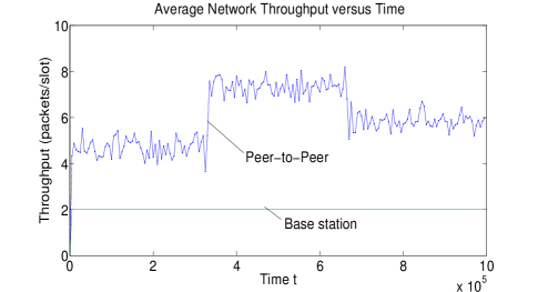
Figure 1: Average throughput per-user versus time.

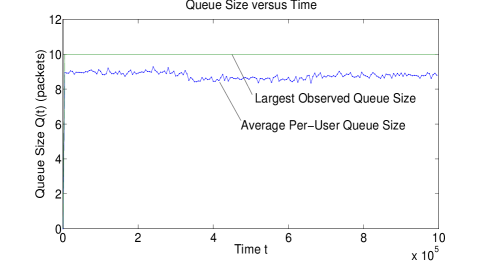
Figure 2: Average and worst-case queue backlog per user versus time.

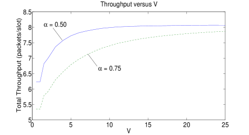
Figure 3: Throughput versus $V$ for $\alpha=0.5$ and $\alpha=0.75$.

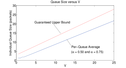
Figure 4: Queue backlog versus $V$, demonstrating the $O(V)$ behavior. The results for $\alpha=0.5$ and $\alpha=0.75$ are right on top of each other. The upper bound $V+3$ is also plotted.

VII Conclusions

This paper develops a simple peer-to-peer scheduling algorithm for a mobile wireless network. Users can opportunistically grab packets from their peers who already have the desired file in their cache. This capability significantly increases the throughput capabilities in the network in comparison to a network where users can only download data from a base station. Our simulations demonstrate these gains, and illustrate that the algorithm is robust to non-ergodic events. Analytically, we have shown that if each user requires a single file with infinite length, then the algorithm can achieve throughput utility that is arbitrarily close to optimality. Distance to optimality depends on a $V$ parameter that also affects an $O(V)$ tradeoff in virtual queue sizes. Our model embeds tit-for-tat constraints directly into the stochastic network optimization problem. This incentivizes participation and naturally leads to an algorithm with reputation queues. Peer-to-peer links between users are favored according to the differential reputation of the users. Finally, while our results were developed for wireless scenarios, we note that the algorithm is general and the techniques can be used in other contexts, such as in wireline computer networks and mixed wireless and wireline networks.

Appendix — Proof of Lemma 4

Here we prove Lemma 4. We state the lemma again for convenience:

Lemma: If all utility functions have right-derivatives bounded by finite constants $\nu_{k}>0$, if $\beta_{k}>0$ for all $k\in{{\cal{K}}}$, and if initial backlog satisfies $Q_{k}(0)=H_{k}(0)=0$ for all $k\in{{\cal{K}}}$, then there are finite constants $C_{1}$ and $C_{2}$, both independent of $V$, such that:

$$||{{\boldsymbol{\Theta}}(t)}||\leq C_{1}+C_{2}V\>\>\forall t\in\{0,1,2,\ldots\}$$

where $||{{\boldsymbol{\Theta}}(t)}||$ is defined:

$$||{{\boldsymbol{\Theta}}(t)}||\leq\sqrt{\sum_{k\in{{\cal{K}}}}H_{k}(t)^{2}+\sum_{k\in{{\cal{K}}}}Q_{k}(t)^{2}}$$

The constants $C_{1}$ and $C_{2}$ are explicitly computed in (30) and (31) below, in terms of the $B$ constant from Lemma 1.

Proof:

Because our algorithm makes decisions for $(\mu_{kb}(t))$ and $\gamma_{k}(t)$ that minimize the last three terms in the right-hand-side of (17) over all alternative feasible decisions, they give a value that is less than or equal to the value when the corresponding terms use the alternative feasible decisions $\tilde{\gamma}_{k}(t)=\tilde{\mu}_{kb}(t)=0$. Thus:

$$\Delta(t)-V\sum_{k\in{{\cal{K}}}}\phi_{k}(\gamma_{k}(t)) \leq B(t)-V\sum_{k\in{{\cal{K}}}}\phi_{k}(0)$$

$$-\sum_{k\in{{\cal{K}}}}H_{k}(t)\beta_{k}$$

$$\leq B-\beta_{min}||{{\boldsymbol{H}}(t)}||$$

where $B$ is the constant that upper bounds $B(t)$ from Lemma 1 for all $t$, $\beta_{min}\mbox{\raisebox{-1.29167pt}{$\overset{\vartriangle}{=}$}}\min_{k\in{{\cal{K}}}}\beta_{k}$, and we have used the fact that $\sum_{k\in{{\cal{K}}}}H_{k}(t)\geq||{{\boldsymbol{H}}(t)}||$. Now define $C_{0}\mbox{\raisebox{-1.29167pt}{$\overset{\vartriangle}{=}$}}\sum_{k\in{{\cal{K}}}}[\phi_{k}(x_{k}^{max})-\phi_{k}(0)]$. We have for all $t$:

$$\Delta(t)\leq B+VC_{0}-\beta_{min}||{{\boldsymbol{H}}(t)}||$$

Note that:

$$\Delta(t)=\frac{1}{2}||{{\boldsymbol{\Theta}}(t+1)}||^{2}-\frac{1}{2}||{{\boldsymbol{\Theta}}(t)}||^{2}$$

Thus:

$$||{{\boldsymbol{\Theta}}(t+1)}||^{2}-||{{\boldsymbol{\Theta}}(t)}||^{2}\leq 2(B+VC_{0})-2\beta_{min}||{{\boldsymbol{H}}(t)}||$$ (26)

Note by Lemma 2 that for all slots $t$, we have $0\leq Q_{k}(t)\leq Q_{max}$, where:

$$Q_{max}\mbox{\raisebox{-1.29167pt}{$\overset{\vartriangle}{=}$}}\nu_{max}V+x_{max}$$

where $\nu_{max}\mbox{\raisebox{-1.29167pt}{$\overset{\vartriangle}{=}$}}\max_{k\in{{\cal{K}}}}\nu_{k}$ and $x_{max}\mbox{\raisebox{-1.29167pt}{$\overset{\vartriangle}{=}$}}\max_{k\in{{\cal{K}}}}x_{k}^{max}$. Thus, for any slot $t$:

$$||{{\boldsymbol{\Theta}}(t)}|| \leq ||{{\boldsymbol{Q}}(t)}||+||{{\boldsymbol{H}}(t)}||$$ (27)

$$\leq Q_{max}\sqrt{K}+||{{\boldsymbol{H}}(t)}||$$

Now suppose that on slot $t$, we have:

$$||{{\boldsymbol{\Theta}}(t)}||>\frac{B+VC_{0}}{\beta_{min}}+Q_{max}\sqrt{K}$$ (28)

Combining this with (27) shows that if (28) holds, then:

$$||{{\boldsymbol{H}}(t)}||>\frac{B+VC_{0}}{\beta_{min}}$$ (29)

It follows that if (28) holds, then (by combining (26) and (29)):

$$||{{\boldsymbol{\Theta}}(t+1)}||^{2}-||{{\boldsymbol{\Theta}}(t)}||^{2}<0$$

Thus, $||{{\boldsymbol{\Theta}}(t)}||$ cannot increase if (28) holds on slot $t$. Because the initial queue backlog is less than the threshold given in (28), it follows that for all $t$:

$$||{{\boldsymbol{\Theta}}(t)}||\leq\frac{B+VC_{0}}{\beta_{min}}+Q_{max}\sqrt{K}+g$$

where $g$ is defined as the maximum possible increase in $||{{\boldsymbol{\Theta}}(t)}||$ in one slot. Because both $Q_{k}(t)$ and $H_{k}(t)$ can increase by at most $x_{max}$ in one slot, we have $g\leq x_{max}\sqrt{2K}$. Thus, for all slots $t$ we have:

$$||{{\boldsymbol{\Theta}}(t)}|| \leq \frac{B+VC_{0}}{\beta_{min}}+(V\nu_{max}+x_{max})\sqrt{K}$$

$$+x_{max}\sqrt{2K}$$

$$\leq C_{1}+C_{2}V$$

where:

$$C_{1} \overset{\vartriangle}{=} B/\beta_{min}+x_{max}(\sqrt{K}+\sqrt{2K})$$ (30)

$$C_{2} \overset{\vartriangle}{=} C_{0}/\beta_{min}+\nu_{max}\sqrt{K}$$ (31)

∎

References

• [1] M.Β J. Neely and L.Β Golubchik. Utility optimization for dynamic peer-to-peer networks with tit-for-tat constraints. Proc. IEEE INFOCOM, 2011.
• [2] L.Β Buttyan and J.-P. Hubaux. Stimulating cooperation in self-organizing mobile ad hoc networks. ACM/Kluwer Mobile Networks and Applications (MONET), vol. 8, no. 5, pp. 579-592, Oct. 2003.
• [3] J.Β Crowcroft, R.Β Gibbens, F.Β Kelly, and S.Β Ostring. Modeling incentives for collaboration in mobile ad-hoc networks. presented at the 1st Int. Symp. Modeling and Optimization in Mobile, Ad-Hoc, and Wireless Networks (WiOpt ’03), Sophia-Antipolis, France, March 2003.
• [4] M.Β J. Neely. Optimal pricing in a free market wireless network. Wireless Networks, vol. 15, no. 7, pp. 901-915, October 2009.
• [5] S.Β Jun and M.Β Ahamad. Incentives in bittorrent induce free riding. In The 3rd ACM SIGCOMM Workshop on Economics of Peer-to-Peer Systems (P2PECON), Philadelphia,PA, August 2005.
• [6] A.Β R. Bharambe, C.Β Herley, and V.Β N. Padmanabhan. Analyzing and improving bittorrent performance. In The 25th Conference on Computer Communications (INFOCOM), Barcelona, Catalunya, Spain, April 2006.
• [7] Karthik Tamilmani, Vinay Pai, and AlexanderΒ E. Mohr. Swift: A system with incentives for trading. In P2PECON, 2004.
• [8] M.Β Piatek, T.Β Isdal, T.Β Anderson, A.Β Krishnamurthy, and A.Β Venkataramani. Do incentives build robustness in bittorrent? In The 4th USENIX Symposium on Networked Systems Design & Implementation (NSDI ), Cambridge, MA, April 2007.
• [9] W.-C. Liao, F.Β Papadopoulos, and K.Β Psounis. Performance analysis of bittorrent-like systems with heterogeneous users. In Performance, 2007.
• [10] Lian, Peng, Yang, Zhang, Dai, and Li. Robust incentives via multi-level tit-for-tat. In IPTPS, 2006.
• [11] Freedman, Aperjis, and Johari. Prices are right: Managing resources and incentives in peer-assisted content distribution. In IPTPS, 2008.
• [12] L.Β Tassiulas and A.Β Ephremides. Stability properties of constrained queueing systems and scheduling policies for maximum throughput in multihop radio networks. IEEE Transacations on Automatic Control, vol. 37, no. 12, pp. 1936-1948, Dec. 1992.
• [13] L.Β Georgiadis, M.Β J. Neely, and L.Β Tassiulas. Resource allocation and cross-layer control in wireless networks. Foundations and Trends in Networking, vol. 1, no. 1, pp. 1-149, 2006.
• [14] F.Β Kelly. Charging and rate control for elastic traffic. European Transactions on Telecommunications, vol. 8, no. 1 pp. 33-37, Jan.-Feb. 1997.
• [15] M.Β J. Neely. Stochastic Network Optimization with Application to Communication and Queueing Systems. Morgan & Claypool, 2010.