Interlayer couplings and the coexistence of antiferromagnetic and d-wave pairing order in multilayer cuprates

Abstract

A more extended low density region of coexisting uniform antiferromagnetism and d-wave superconductivity has been reported in multilayer cuprates, when compared to single or bilayer cuprates. This coexistence could be due to the enhanced screening of random potential modulations in inner layers or to the interlayer Heisenberg and Josephson couplings. A theoretical analysis using a renormalized mean field theory, favors the former explanation. The potential for an improved determination of the antiferromagnetic and superconducting order parameters in an ideal single layer from zero field NMR and infrared Josephson plasma resonances in multilayer cuprates is discussed.

I Introduction

Although the cuprate superconductors have been studied for a quarter century, the exact form of the interplay of antiferromagnetic(AF) and d-wave pairing(dSC) order at low hole doping is not known reliably. Experiments on very low doped cuprates show insulating behavior and a critical hole concentration, $x_{c}$, for the onset of superconductivity. The presence of a strongly varying potential due to the random distributions of the acceptors is believed to be important at very low hole densities. There are reports of a spin glass phase separating the AF and dSC regions of the phase diagram review . A series of neutron scattering experiments on La_2-xSr_xCuO₄ found stripe order but with a change of orientation from parallel to the Cu-O-Cu bonds at $x>x_{s}$ to a $45^{\circ}$ direction at $x<x_{s}$ waki . Neutron scattering experiments on YBa₂Cu₃O_6+y found spin density wave (SDW) order in the hole concentration range 0.05$<x<0.08$haug . On the other hand coexistence of uniform AF order with dSC has been deduced from NMR studies of multilayer Hg- and Ba₂Ca₃Cu₄O₈(F_yO_1-y)₂-cuprates in a substantially larger hole density rangekitaoka1 . In this paper we analyse the role of AF and dSC interlayer coupling in multilayer cuprates and their effect on the coexistence on AF and dSC order.

The observation by Kitaoka, Mukuda and collaborators kitaoka1 of substantial zero magnetic field shifts on a unique Cu-site in the innermost layers led them to claim uniform AF order in underdoped layers with $x\sim 0.1$. The multilayer cuprates are doped by acceptors in the insulating blocks between the multilayer blocks, but their random potential will be weakened in the inner layers due to screening by the more highly doped metallic outer layers. Thus these multilayer cuprates offer the best possibility to reliably determine AF and dSC ordering at low doping in a clean single layer. In this paper we illustrate the potential of multilayer systems by considering the case of 4-layer cuprates for which experimental results exist in a wide density range. Variational Monte Carlo calculations for an ideal single layer strong coupling t-J model find a substantial coexistence region of spatially uniform AF and dSC order up to a critical hole density $x\sim 0.1$ ogata . Theoretical support for dSC order at low doping in a single layer also comes from exact diagonalization studies on clusters of the t-J model containing up to 32-sites doped with 2 holes Leung . When extrapolated to an infinite layer, these point to a robust d-wave cooperon ( bound hole pair ) resonance at low doping . The virtual exchange of cooperons will act as a pairing mechanism for doped holes in near nodal states at low hole densities, in the presence of strong AF local (and probably long range) order Rice .

The two order parameters to be determined are the sublattice magnetization of AF order and the pairing amplitude of dSC ordering. The former is directly measured by the zero field shift on Cu-sites in NMR experiments. kitaoka1 In multilayer samples the Josephson couplings between the dSC order in neighboring layers lead to the Josephson plasma resonances which appear in infrared spectra with the electric field oriented along the c-axis Marel . The energies of these resonances are proportional to the product of the dSC order parameters. The combination of these two measurements on the same samples can, in principle, be used to determine the values and the dependence of both AF and dSC order parameters on the hole density. To obtain information on the interplay of AF and dSC order in a single layer, we need to include the effects of interlayer couplings between the respective order parameters in the analysis. Note, the interlayer spin coupling disfavors SDW order in adjacent planes with different hole densities and therefore different periodicities. As a result we restrict our attention to the case of commensurate AF and dSC order.

In this paper we report on calculations using the renormalized mean field theory (RMFT), a method introduced in the early days by Zhang and collaborators RMFT , to treat the strong coupling t-J model. We extend the method to multilayer t-J models. RMFT calculationsstripe-rvb generally agree well with more accurate variational Monte-Carlo calculations VMC in the case of a single layer.

To treat multilayer materials we require the values of the interlayer couplings. The Heisenberg spin-spin coupling has been directly measured with a strength typically of order a tenth of the intralayer coupling. The interlayer Josephson coupling constants are less well known, as will be discussed further below.

A second key input is the value of the hole densities in inequivalent layers. Kitaoka and collaborators have measured the Cu-Knight shift in each layer and used the room temperature value as input in an empirical formula to estimate the hole density in each layer. We shall return to these inputs below.

II $t-J$ Model for multilayer cuprates

We start by defining the t-J model for a single plane. $H_{l}^{t-J}$ for the $l^{th}$ layer is given by

$$H^{t-J}_{l} =-\sum_{ij\sigma}P_{G}t_{ij}c_{l,i\sigma}^{{\dagger}}c_{l,j\sigma}P_{G}+J\sum_{\left\langle ij\right\rangle}\mathbf{S}_{l,i}\cdot\mathbf{S}_{l,j},$$ (1)

where $c_{il\sigma}$ is an annihilation operator of a spin $\sigma$ electron at site $i$ in layer $l$, $P_{G}$ is the Gutzwiller projection operator which enforces the no-double occupancy condition in cuprates, $t_{ij}$ is the hopping integral between site i and site j with nearest neighbor hopping $t_{NN}=t$, next nearest neighbor hopping $t_{NNN}=t^{\prime}$, and $t_{ij}=0$ for the remaining site pairs. J is the superexchange coupling between NN sites.

The interlayer coupling, $H_{lm}$, between two neighboring layers $l$ and $m$ includes a superexchange spin-spin coupling and an interlayer hopping term. The interlayer superexchange coupling is given by

$$H_{lm}^{J}=J_{\perp}\sum_{i}\mathbf{S}_{l,i}\cdot\mathbf{S}_{m,i},$$ (2)

and the interlayer hopping term reads

$$H^{t}_{lm} =P_{G}\sum_{\mathbf{k}}t_{\perp}(\mathbf{k})(c_{l,\mathbf{k}\sigma}^{{\dagger}}c_{m,\mathbf{k}\sigma}+h.c.)P_{G},$$ (3)

whereinterlayer $t_{\perp}(\mathbf{k})=t_{\perp}\phi^{2}_{\mathbf{k}}/2$, with $\phi_{\mathbf{k}}=\cos k_{x}-\cos k_{y}$.

In a system with more than two layers, the hole concentrations on two adjacent inequivalent layers are different and the Fermi surfaces of the two layers are mismatched. Because planar momentum is conserved in interlayer hopping, the mismatch of the Fermi surfaces means that direct interlayer single particle hopping and interlayer pairing can be neglected. However a Cooper pair can tunnel from the Fermi surface of one layer into a pair state off the Fermi surface on a neighboring layer, conserving the planar momentum of the individual electrons, This process can be written down in standard perturbation theory as

$$H^{\Delta}_{lm} =-\sum_{\mathbf{k}}\frac{t_{\perp}^{2}\phi^{4}_{\mathbf{k}}}{2\omega_{c}}$$

$$\phantom{=-}\times P_{G}\left(c_{l,-\mathbf{k}\downarrow}^{{\dagger}}c_{l,\mathbf{k}\uparrow}^{{\dagger}}c_{m,\mathbf{k}\uparrow}c_{m,-\mathbf{k}\downarrow}+h.c.\right)P_{G}$$ (4’)

with $\omega_{c}$ a characteristic energy. This excited state Cooper pair can subsequently relax to the Fermi surface of the second layer through interactions such as the J-term in the single plane Hamiltonian. This virtual tunneling process through pair states off the Fermi energy will be the leading contribution of the interlayer Josephson coupling, arising from Cooper pair hopping between inequivalent layers leading to an interlayer Josephson coupling

$$H^{\Delta}_{lm} =\sum^{\prime}_{\mathbf{k}\mathbf{k}^{\prime}}\frac{t_{\perp}^{2}\phi^{4}_{\mathbf{k}}J(\mathbf{k}-\mathbf{k}^{\prime})}{2\omega_{c}\omega^{\prime}_{c}}$$

$$\phantom{=-}\times P_{G}\left(c_{l,-\mathbf{k}\downarrow}^{{\dagger}}c_{l,\mathbf{k}\uparrow}^{{\dagger}}c_{m,\mathbf{k^{\prime}}\uparrow}c_{m,-\mathbf{k^{\prime}}\downarrow}+h.c.\right)P_{G},$$ (4)

where $J(\mathbf{q})=J(\cos q_{x}+\cos q_{y})$ is the pair hopping amplitudes, $\omega^{\prime}_{c}$ is a characteristic energy related to the intralayer relaxation process, and the prime on the summation denote s that the summation are only in the vicinity of Fermi surfaces with cut-off $\omega_{D}$.

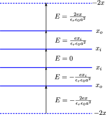
Figure 1: Schematic illustration for the hole carrier charge distribution $x$, electric field $\vec{E}$ (direction indicated by arrows) in 4-layer Cu-oxides. Horizontal lines represent layers. Sub-indices $i$ and $o$ represent inner and outer planes, respectively. The top and bottom dashed lines represent chemically doped charge.

In multilayer materials the distribution of hole densities on the individual layers plays an important role. Theoretical estimates of the hole densities can be made using a Hartree approximation scheme by including the electrostatic energy in the Hamiltonian electrostatic . For simplicity, we consider each layer as an infinite plane with homogeneous charge. The electric field generated by such a plane is $E=\frac{\rho}{2\epsilon_{r}\epsilon_{0}}=\frac{ex}{2\epsilon_{r}\epsilon_{0}a^{2}}$, where $\epsilon_{r}$ is the relevant dielectric constant, $x$ is the hole concentration of the layer, and $a$ is the lattice constant. For a 4-layer system, we denote $x_{o}$ and $x_{i}$ as the hole concentrations of the outer layers and the inner layers, respectively. The average hole concentration is $x=(x_{o}+x_{i})/2$, while the electron concentration of the acceptor layer above and below the 4-layers is $2x$. The spatial distribution of electric field is depicted in fig. 1. We are only interested in the terms relevant to the charge inhomogeneity, so the electrostatic energy between acceptor layer and outer layer can be ignored. Then the electrostatic energy per plaquette in the 4-layer case is $E_{es}=\frac{e^{2}x_{i}^{2}d}{\epsilon_{r}\epsilon_{0}a^{2}}$, where $d$ is the distance between two adjacent CuO₂ layers. The Hamiltonian for multilayer system then reads

$$H =\sum_{l}H_{l}^{t-J}+\sum_{\left\langle lm\right\rangle}(H^{\Delta}_{lm}+H^{J}_{lm})+E_{es}.$$ (5)

The dielectric screening of the interlayer electric field arises from displacements of the ionic layer between the neighboring layers and is not identical to the static c-axis dielectric screening due to optical phonons etc. We adjust the value of $\epsilon_{r}$ to fit the estimated values for the layer densities (see below).

III Renormalized mean field theory for multilayer system

In this section, we will use RMFT to analyse the multi-layer Hamiltonian. The main element of the RMFT theory is the so-called Gutzwiller approximation, which replaces the Gutzwiller projection in the Hamiltonian by simple numerical factors. Let $\left\langle\hat{O}\right\rangle$ and $\left\langle\hat{O}\right\rangle_{0}$ be the average values of operator $\hat{O}$ in the Gutzwiller projected state and in the unprojected state, respectively, then $\left\langle\hat{O}\right\rangle\approx g_{o}\left\langle\hat{O}\right\rangle_{0}$, with $g_{o}$ a numerical factor, depending on the hole density and the process associated with the operator $\hat{O}$. The coexistence of AF and dSC order in the t-t’-J model for a single layer material has been investigated within RMFT recently by K.-Y. Yang et al. stripe-rvb . Here we generalize their calculations to a multilayer system. Note that in the RMFT the superconducting order parameter is non-zero at wave-vector off the Fermi surface. The virtual tunneling process through pair states off the Fermi energy when the two layers have different hole concentrations we discussed in Section II may also be taken into account by including the pair scattering on the same layer along with the second order interlayer hopping process conserving momentum of single electrons. Below we shall use Eq. (4’) for the interlayer tunneling directly to study the multi-layer system described in Eq. (5).

We now introduce the following mean fields

$$\Delta_{0,l} =\frac{1}{4N}\sum_{i}\left\langle\sum_{\delta=\pm\hat{x}}c_{l,i\uparrow}c_{l,i+\delta\downarrow}-\sum_{\delta=\pm\hat{y}}c_{l,i\uparrow}c_{l,i+\delta\downarrow}\right\rangle_{0}$$

$$m_{0,l} =\frac{1}{N}\sum_{i}(-1)^{i}\left\langle S_{l,i}^{z}\right\rangle=\frac{1}{2N}\sum_{i\sigma}\sigma(-1)^{i}\left\langle c_{l,i\sigma}^{{\dagger}}c_{l,i\sigma}\right\rangle_{0}$$

$$\chi_{0,l,ij,\sigma} =\left\langle c_{l,i\sigma}^{{\dagger}}c_{l,j\sigma}\right\rangle_{0},$$ (6)

where $\left\langle\right\rangle_{0}$ indicates average with the unprojected state. Since we are only interested in the ground state, we can assume that the mean fields $\Delta_{0,l}$ are all real. In the presence of AF order, the magnetization on the sublattices A and B are opposite, and the mean fields $\chi_{0,l,ij,\sigma}$ from NNN sites depend on the sublattice and spin. We introduce the following mean fields, $\chi_{0,l,AA,\sigma}=\frac{1}{2N}\sum_{i\in A}\sum_{j=NNN(i)}\chi_{0,l,ij,\sigma}$ and $\chi_{0,l,BB,\sigma}=\frac{1}{2N}\sum_{i\in B}\sum_{j=NNN(i)}\chi_{0,l,ij,\sigma}$. Since $\chi_{0,l,AA,\sigma}=\chi_{0,l,BB,-\sigma}$, we can further simplify the notation as $\chi_{0,l,AA}=\chi_{0,l,AA,\uparrow}$ and $\chi_{0,l,BB}=\chi_{0,l,BB,\uparrow}$. On the other hand, the mean fields $\chi_{0,l,ij,\sigma}$ for NN sites are independent of the sublattice $ij$ and spin $\sigma$, so we can set the mean fields $\chi_{0,l,AB}=\frac{1}{8N}\sum_{i\sigma}\sum_{j=NN(i)}\chi_{0,l,ij,\sigma}$. The hole concentration on each layer satisfies the condition.

$$x_{l} =1-\left\langle n_{l}\right\rangle=1-\frac{1}{N}\sum_{i\sigma}\left\langle c_{l,i\sigma}^{{\dagger}}c_{l,i\sigma}\right\rangle.$$ (7)

Then we consider the Gutzwiller factors. In intralayer terms, we adopt the same form of the factors $g_{l,AB}^{t},g_{l,AA}^{t},g_{l,BB}^{t},g_{l}^{m},g_{l}^{xy}$, and $g_{l}^{z}$ as used previously for the single layer t-J model stripe-rvb . For the interlayer hopping and superexchange coupling terms, we make a simple assumption that the Gutzwiller factors are $g_{lm}^{t}=\sqrt{g^{t}_{l,AB}g^{t}_{m,AB}}$ and $g^{z}_{lm}=\sqrt{g^{m}_{l}g^{m}_{m}}$, respectively. The total energy reads

$$E =\sum_{l}E_{l}+\sum_{\left\langle lm\right\rangle}E_{lm}+E_{es},$$ (8)

where $E_{l}$ is given by the RMFT for single layer t-t’-J model stripe-rvb , the electrostatic energy $E_{es}$ is specified in the previous section, and the interlayer energy $E_{lm}$ takes the form

$$E_{lm} =\frac{\left\langle H_{lm}^{\Delta}+H^{J}_{lm}\right\rangle}{N}=-4(g^{t}_{lm})^{2}\frac{t_{\perp}^{2}}{4N\omega_{c}}\sum_{\mathbf{k}}^{\prime}\phi_{\mathbf{k}}^{4}\bigl{(}\Delta_{0,l,\mathbf{k}}\Delta_{0,m,\mathbf{k}}$$

$$\phantom{=}+\Delta_{0,l,\mathbf{k+Q}}\Delta_{0,m,\mathbf{k+Q}}\bigr{)}+J_{\perp}g^{z}_{lm}m_{0,l}\bar{m}_{m},$$ (9)

with $\Delta_{0,l,\mathbf{k}}=\left\langle c_{\mathbf{k}\uparrow}^{l}c_{-\mathbf{k}\downarrow}^{l}\right\rangle_{0}$. Note that the magnetic moment $m_{l}$ and superconducting order parameter $\Delta_{l}$ are related to the mean fields by the Gutzwiller renormalization factorsRMFT ,

$$m_{l} =\sqrt{g^{z}_{l}}m_{0,l} \Delta_{l} =g^{t}_{l,AB}\Delta_{0,l}.$$ (10)

These approximations lead to the mean field Hamiltonian

$$H_{MF} =\sum_{l\mathbf{k}\sigma}\left(\epsilon_{l,\mathbf{k}}c_{l,\mathbf{k}\sigma}^{{\dagger}}c_{l,\mathbf{k}\sigma}-\sigma M_{l,\mathbf{k}}c_{l\mathbf{k}\sigma}^{{\dagger}}c_{l,\mathbf{k+Q}\sigma}\right)$$

$$\phantom{=}-\sum_{l\mathbf{k}\sigma}\left(V_{l,\mathbf{k}}c_{l,-\mathbf{k}\downarrow}c_{l,\mathbf{k}\uparrow}+h.c.\right),$$ (11)

where

$$\epsilon_{l,\mathbf{k}} =\frac{\partial E}{4\chi_{0,l,AB}}\gamma_{\mathbf{k}}+\frac{1}{2}\left(\frac{\partial E}{\partial\chi_{0,l,AA}}+\frac{\partial E}{\partial\chi_{0,l,BB}}\right)\theta_{\mathbf{k}}-\tilde{\mu}_{l}$$

$$M_{l,\mathbf{k}} =-\frac{1}{2}\left(\frac{\partial E}{\partial\chi_{0,l,AA}}-\frac{\partial E}{\partial\chi_{0,l,BB}}\right)\theta_{\mathbf{k}}-\frac{1}{2}\frac{\partial E}{\partial m_{0,l}}$$

$$V_{l,\mathbf{k}} =\frac{1}{4}\frac{\partial E_{l}}{\partial\Delta_{0,l}}\phi_{\mathbf{k}}+\frac{N}{2}\sum_{m}\frac{\partial E_{lm}}{\partial\Delta_{0,l,\mathbf{k}}}$$

$$\tilde{\mu}_{l} =\frac{\partial E}{\partial x_{l}}+\mu,$$ (12)

and $\gamma_{\mathbf{k}}=\cos k_{x}+\cos k_{y}$, and $\theta_{\mathbf{k}}=\cos k_{x}\cos k_{y}$.

IV Results and Discussions

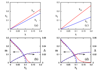
Figure 2: The order parameters and hole concentrations calculated in 4-layer t-t’-J model Eq. (5). Model parameters are $J=0.3t$, $t^{\prime}=-0.3t$, interlayer pair hopping $t_{\perp}^{2}/\omega_{c}=0.1t$, interlayer spin coupling $J_{\perp}=0.1J$. Upper panel: the hole concentrations for each layer $x_{l}$ vs average hole concentrations $x$. Thick blue curves are for inner layer ($x_{i}$), thin red for outer layer ($x_{o}$). Lower panel: magnetic moment $m$ and superconducting order parameter $\Delta$ as function of hole doping for each layers $x_{l}$. Thick blue curves are for inner layer, thin red for outer layer. Left panel: dielectric constant $\epsilon=200$, right panel: $\epsilon=50$. Dashed curves in (b) and (d) are for single layer results, plotted for comparison.

The mean field energy defined by Eqn (8) has been minimized numerically for the case of 4-layers. The results depend on the hole densities which in turn depend on the value of the dielectric constant, $\epsilon_{r}$. In fig. 2, the two upper figures show the density in each layer as function of the total doping for two choices $\epsilon_{r}=200$ and $\epsilon_{r}=50$. The lower figures show the resulting values of the order parameters in each layer. The single layer result is also shown in the figure as a dashed line for comparison. The SC order parameters of the 4-layer system and single layer system are almost equal and independent of $\epsilon_{r}$. This is a consequence of the weak Josephson coupling between adjacent layers in the multilayer system due to the mismatch of the Fermi surfaces and the suppression of the interlayer hopping by the strong onsite Coulomb interaction.

Table 1: Comparison between NMR experimental results on Ba₂Ca₃Cu₄O₈(F_yO_1-y)₂kitaoka1 and the renormalized mean field theory for 4-layer $t-t^{\prime}-J$ model. $y$ is the content of $F$ in the compound. $x_{op}$ and $x_{ip}$ are the hole concentrations on the outer and inner planes. $m_{op}$ and $m_{ip}$ are the AF magnetic moment on the outer and inner planes, respectively. $\epsilon$ is the fitted value of the dielectric constant from the hole distribution. $\omega_{ii}$ and $\omega_{io}$ are the Josephson plasma frequencies between two inner layers and between inner layer and outer layer, respectively.

y	NMR Exp.				Theory
	$x_{op}$	$m_{op}$	$x_{ip}$	$m_{ip}$	$\epsilon$	$m_{op}$	$m_{ip}$	$\omega_{io}$	$\omega_{ii}$
0.6	0.141	0	0.089	0	87	0.010	0.096	492	394
0.7	0.111	0	0.074	0.04	107	0.043	0.137	399	322
0.8	0.092	0	0.069	0.06	170	0.093	0.150	348	301
1	0.073	0.055	0.059	0.09	247	0.138	0.173	278	243

The interlayer AF coupling slightly enhances the AFM moment and critical doping $x_{c}$ of the inner layers and leads to a finite AFM moment on the outer layers when their hole concentration is much larger than the single layer critical doping $x_{c}$. Such a long tail arises because of the lower hole concentration on the inner layers. A smaller $\epsilon_{r}$ leads to larger charge imbalance between the outer and inner layers and so to larger $x_{c}$ of outer layers, as shown in fig. 2. If one neglects the long tail of the AFM moment of the outer layers, the phase diagram of multi-layer system is very similar with that of a single layer system, independent of the value of the dielectric constant $\epsilon_{r}$. This indicates that experiments on multilayer system can capture the essential physics of single layer t-J model

We turn now to the relation of the model with experiment. The two order parameters we investigated above are the AFM magnetization and the pairing amplitude of dSC ordering. The former has been directly measured by the zero field shift in NMR. In the NMR experiments, Shimizu, Kitaoka and collaborators kitaoka2 have also used an empirical scaling of the Cu Knight shift, measured at room temperature, to deduce hole densities of individual layers. Note this scaling form has evolved with time. In tab. 1, we show the value of the relative dielectric needed to fit the charge distribution recently determined from NMR experiments on the 4-layer Ba₂Ca₃Cu₄O₈(F_yO_1-y)₂ cuprate. Note, in these oxy-fluoride cuprates the hole density differs substantially from the nominal F- concentration,y. Though the dielectric constant required to fit the hole density changes from 87 to 247 as the total hole density decreases from 0.46 to 0.264, the physics in each layer should not change very much as analyzed above. In Table 1, we also show the AFM moments calculated by the RMFT and measured by NMR experiments. The former values are considerably larger than the latter, indicating an over estimation of the AFM order in the RMFT theory. The comparison between theory and experiment is sensitive to the values of the hole density. For example, if we scale the value of the estimated hole density so that the optimal density with the highest Tc for a single layer is $(x_{c}=0.2)$ rather $(x_{c}=0.16)$ quoted in Mukuda et al.kitaoka1 ; kitaoka2 , this leads to an increase in the input values for the hole density in the RMFT calculations by a factor of 1.25. Then the calculated values of the AF moment shown in Tab 1, are smaller, although still too big, and in better agreement with experiment.

Turning to the dSC ordering, as mentioned earlier the pairing amplitudes enter into the Josephson plasma frequencies observed in the infrared spectra with the electric field oriented along the c-axis. In multilayer cuprates, there are two kinds of Josephson plasma frequencies which correspond to inter-multilayer and intra-multilayer Josephson couplings respectively. In this paper, we are only interested the latter, i.e. the Josephson plasma frequencies related to the Josephson coupling between two adjacent CuO₂ layers in same unit cell. The Josephson energy between those two layers can be written as $E_{J}=-J_{lm}\cos(\phi_{l}-\phi_{m})$, where $\phi_{l}$ and $\phi_{m}$ are the phase of the superconducting order parameter of the two layers respectively. For the two layers with the same hole concentration, $J_{lm}$ is given in our RMFT by,

$$J_{lm} =\frac{2}{\beta N}\sum^{\prime}_{\mathbf{k}}\sum_{i\omega_{n}}(g^{t}_{lm})^{2}t^{2}_{\perp}(\mathbf{k})\Bigl{|}\mathcal{F}_{l}(\mathbf{k},i\omega_{n})\Bigl{|}\mathcal{F}^{{\dagger}}_{m}(\mathbf{k},i\omega_{n})$$

$$\phantom{\propto}+\Bigl{|}\mathcal{F}_{l}(\mathbf{k+Q},i\omega_{n})\Bigl{|}\mathcal{F}^{{\dagger}}_{m}(\mathbf{k+Q},i\omega_{n})\Bigr{|}=t_{\perp}^{2}\tilde{\omega}^{2}_{lm},$$ (13)

where $\mathcal{F}_{l}$ is the anomalous Green’s function of layer $l$, $i\omega_{n}$ is the Matsubara frequency, $\mathbf{Q}=(\pi,\pi)$, and $\sum^{\prime}$ indicates the summation is only over the reduced zone. The Josephson plasma frequency which corresponds to the Josephson coupling between those two layers is proportional to the Josephson coupling constant Leggett ; Marel , i.e. $\omega^{J}_{lm}\propto\sqrt{J_{lm}}$. So we have

$$\omega^{J}_{lm} =C\tilde{\omega}_{lm},$$ (14)

where $C$ is a constant related to $t_{\perp}$ and finite frequency dielectric constant $\epsilon(\omega_{J})$. For simplicity, we can assume that $C$ is weakly dependent on the hole concentrations and materials.

For a 4-layer material, there are two intra-unit cell Josephson plasmon frequencies $\omega_{io}$ and $\omega_{ii}$ which correspond to the Josephson coupling between two inner layers and between the inner and outer layers respectively. A recent optical experiment on a 4-layer Hg-based compound has shown that the Josephson plasmon frequencies are 360 cm^-1 for inner layers and 540 cm^-1 for outer and inner layers respectively leading to a ratio of $1.5$uchida . According to eqn. (14), $\omega_{io}/\omega_{ii}=\tilde{\omega}_{io}/\tilde{\omega}_{ii}$. Using the estimated hole concentrations of the Hg-compound, the ratio calculated with RMFT is around $1.25$ which is fairly close to the experimental value. To make further comparison, we calculate the factor $C$ with $C=\sqrt{\omega_{io}\omega_{ii}/\tilde{\omega}_{io}\tilde{\omega}_{ii}}\approx 10$, where the plasmon frequencies are the experimental values for the Hg-compound and the $\tilde{\omega}$ is calculated with RMFT. Using this estimate for $C$ allows us to obtain values for the plasma frequencies for the 4-layer Ba₂Ca₃Cu₄O₈(F_yO_1-y)₂ material. The results are quoted in Table 1.

V Summary

In this paper we presented a series of calculations using the RMFT to treat the AF and dSC order parameters in 4-layer cuprates. The RMFT calculations/citestripe-rvb and also the results of single VMC calculations/citeVMC, give a more extended region of coexistence of the two order parameters than that observed in single and bilayer cuprates. The extended coexistence region in the 4- layer cuprates agrees with the conclusion of the NMR experiments in the inner layers. In our analysis the extended region comes not from strong interlayer magnetic and Josephson coupling, but from the extended coexistence region already present in single layers in the RMFT approximation. This analysis suggests that the difference in the density range of coexisting order in multilayer cuprates compared to experiments on single and bilayer cuprates, is due to the better screening of the external potential modulation in the inner layers of multilayer cuprates, when compared to single and bilayer cuprates. The latter are adjacent to the random acceptors, while the metallic outer layers screen the random potential at the inner layers. In principle the combination of zero field NMR and infrared Josephson plasma frequencies allows one to determine both AF and dSC order parameters. However, in order to go further and directly compare measured and calculated order parameters a better determination of the interlayer Josephson coupling constant and its variation with the hole densities in the individual layers, is required. To this end a series of measurements of the Josephson plasma frequencies and the AF moments by zero field NMR at different hole densities on the same multilayer material would be helpful.

We acknowledge financial support in part from Hong Kong RGC GRF grant HKU706507, the National Natural Science Foundation of China 10804125, and also from the Swiss Nationalfond and MANEP network.

References

- (1) For a review see M.-H.Julien, Physica B 329-333, 693 (2003)
- (2) S. Wakimoto, R. J. Birgeneau, M. A. Kastner, Y. S. Lee, R. Erwin, P. M. Gehring, S. H. Lee, M. Fujita, K. Yamada, Y. Endoh, K. Hirota, and G. Shirane, Phys. Rev. B 61, 3699 (2000)
- (3) D. Haug, V. Hinkov, Y. Sidis, P. Bourges, N. B. Christensen, A. Ivanov, T. Keller, C. T. Lin, and B. Keimer, New J. Phys 12, 105006 (2010)
- (4) M. Ogata and H.Fukuyama, Rep. Prog. Phys. 71, 036501 (2008)
- (5) A. L. Cheryshev, P. W. Leung, and R. J. Gooding, Phys. Rev. B 58, 13594 (1998)
- (6) For a recent review see H. Mukuda, S. Shimizu, A. Iyo, and Y. Kitaoka, J. Phys. Soc. Jpn. 81, 011008 (2012)
- (7) A. J. Leggett, Prog. Theor. Phys. 36, 901-930 (1966)
- (8) D. van der Marel, J. Supercond. 17, 559 (2004)
- (9) F. C. Zhang, C. Gros, T. M. Rice, and H. Shiba, Supercond.Sci.Technol. 1, 36 (1988)
- (10) K.-Y.Yang, W. Q. Chen, T. M. Rice, M. Sigrist, and F. C. Zhang, New J. Phys. 11, 055053 (2009)
- (11) G. J. Chen, R. Joynt, F. C. Zhang, and G. Gros, Phys. Rev. B 42, 2662 (1990);T. Giamarchi and C. Lhuillier, Phys. Rev. B 43, 12943 (1991) ; A. Himeda and M. Ogata, Phys. Rev. B 60, R9935 (1999)
- (12) S. Chakravarty, A. Sudbo, P. W. Anderson, and S. Strong, Science 261, 337 (1993); O. K. Andersen, A. I. Liechtenstein, O. Jepsen, and F. Paulsen, J. Phys. Chem. Solids 56,1573, (1995)
- (13) M. Di Stasio, K. A. Mueller, and L. Pietronero, Phys. Rev. Lett 64, 2827 (1990)
- (14) J. Y. Gan, Y. Chen, Z. B. Su, and F. C. Zhang, Phys. Rev. Lett. 94, 067005 (2005)
- (15) M. Ogata and A. Himeda, J. Phys. Soc. Jpn. 72, 374 (2003)
- (16) S. Shimizu, S. Iwai, S. Tabata, H. Mukuda, Y. Kitaoka, P. M. Shirage, H. Kito, and A. Iyo, Phys. Rev. B 83, 144523 (2011)
- (17) Y. Hirata, K. M. Kojima, S. Uchida, M. Ishikado, A. Iyo, H. Eisaki, and S. Tajima, Physica C: Superconductivity 470, S44 (2010)
- (18) T. M. Rice, K.-Y. Yang, and F. C. Zhang, Rep. Prog. Phys. 75, 016502 (2012)