Exact Eigenvalues of the Pairing Hamiltonian Using Continuum Level Density

Abstract

The pairing Hamiltonian constitutes an important approximation in many- body systems, it is exactly soluble and quantum integrable. On the other hand, the continuum single particle level density (CSPLD) contains information about the continuum energy spectrum. The question whether one can use the Hamiltonian with constant pairing strength for correlations in the continuum is still unanswered. In this paper we generalize the Richardson exact solution for the pairing Hamiltonian including correlations in the continuum. The resonant and non-resonant continuum are included through the CSPLD. The resonant correlations are made explicit by using the Cauchy theorem. Low lying states with seniority zero and two are calculated for the even Carbon isotopes. We conclude that energy levels can indeed be calculated with constant pairing in the continuum using the CSPLD. It is found that the nucleus ²⁴C is unbound. The real and complex energy representation of the continuum is developed and their differences are shown. The trajectory of the pair energies in the continuum for the nucleus ²⁸C is shown.

I Introduction

The approximate BCS solution of the pairing Hamiltonian has been extensively used in Condensed Matter to study pairing correlations in ultra-small metallic grains von Delft et al. (1996); Braun and von Delft (1999). A much better approximation is given by the Density Matrix Renormalization Group Dukelsky and Sierra (1999). But, the pairing Hamiltonian admits an exact solution worked out by Richardson at the beginning of the sixties Richardson (1963); Richardson and Sherman (1964). A more recent derivation of the exact solution can be found in ref. von Delft and Braun (1999). The first application of the Richardson exact solution was done in ultra-small grains system Sierra et al. (1999, 2000). References Sierra et al. (1999, 2000) and von Delft and Braun (1999) marks the resurgence of the Richardson’s exact solution of the pairing Hamiltonian. The acknowledge to Richardson in refs. Sierra et al. (2000); von Delft and Braun (1999) constitutes a recognition to him after forty years in the oblivion.

The Richardson exact solution has been used to study the effect of the resonant single-particle states on the pairing Hamiltonian Hasegawa and Kaneko (2003). In ref. Pittel and Dukelsky (2006) the authors gave an interpretation of the pair energies from the Richardson solution. They relate the pairing correlations with the pair energies distribution in the complex plane. The pairing Hamiltonian is not only exactly soluble but also quantum integrable Cambiaggio et al. (1997); Sierra (2000); Amico et al. (2001); Dukelsky et al. (2001). Besides the constant pairing, a very special kind of separable pairing interaction also admits an exact solution Balantekin and Pehlivan (2007); Dukelsky et al. (2011). A review on exact solutions of the pairing Hamiltonian can be found in the ref. Dukelsky et al. (2004).

The pairing Hamiltonian approximates the influence of the residual interaction acting among the valence states lying close to the Fermi level. However, it is an open question how one must treat pairing in the continuum. Previous studies on the contribution from the continuum to pairing have been reported in refs. Sandulescu et al. (2000); Kruppa et al. (2001); Hasegawa and Kaneko (2003).

In this paper we reformulate the problem of determining the exact eigenenergies of the pairing Hamiltonian when the continuum is included. Real and complex energy representations of the continuum are used. The BCS approximation is not a convenient tool to treat many-body pairing close to the drip line Dobaczewski et al. (1996); Id Betan (2012). It is the intention of this paper to give an exact treatment of the many-body pairing which overcomes the drawbacks of the BCS treatment.

The paper is organized as follows. Section II briefly reviews the derivation of the Richardson equations with the continuum represented on the real energy axis or in the complex energy plane. In Sec. III the low lying states of even Carbon isotopes are evaluated and a comparison of the solutions using the real energy representation are compared with the ones obtained in the complex energy representation. The trajectory of the pair energies are analyzed as a function of the pairing strength. The continuum pair energies are introduced in this section. Finally, Sec. IV summarizes the main results of the paper.

II Method

In this section the Richardson equations for a continuum basis is given. First the continuum is included by enclosing the system in a large spherical box. After the final equations have been obtained, we take the limit of the box to infinity and introduce the single particle level density. In order to avoid the Fermi gas we take the derivative of the phase shift for the continuum part of the single particle level density Beth and Uhlenbeck (1937). Finally, we parametrized the CSPLD for the resonant partial waves and make the analytic continuation to the complex energy plane.

II.1 System in a Box

In this sub-section we follow the derivation of the exact solution as it was given by Jan Von Delft and Fabian Braun in ref. von Delft and Braun (1999). The inclusion of the system in a large spherical box provides a finite discrete set of negative (bound) energies and an infinite discrete set of positive (continuum) energies. Let us called $\varepsilon_{a}$ the discrete energy with degeneracy $2j_{a}+1$, with $\alpha=\{a,m_{\alpha}\}=\{n_{a},l_{a},j_{a},m_{\alpha}\}$. The pairing Hamiltonian is given by,

$$H_{P}=\sum_{\alpha}\;\varepsilon_{a}\;c^{\dagger}_{\alpha}c_{\alpha}-G\sum_{am_{\alpha}>0}\;\sum_{bm_{\beta}>0}c^{\dagger}_{\alpha}c^{\dagger}_{\bar{\alpha}}c_{\bar{\beta}}c_{\beta}\;,$$ (1)

with $c^{\dagger}_{\bar{\alpha}}=(-)^{j_{a}-m_{\alpha}}\;c^{\dagger}_{a-m_{\alpha}}$. We introduce the pair creation operator

$$A^{\dagger}_{a}=\sum_{m_{\alpha}>0}\;c^{\dagger}_{\alpha}\;c^{\dagger}_{\bar{\alpha}}\;,$$ (2)

which creates a pair of time reversal states with quantum number $a$.

Following Von Delft and Braun von Delft and Braun (1999), who were inspired by a suggestion by Richardson, we propose the $N$-body ($N=2N_{\rm pair}$) eigenfunction as the antisymmetrised product of $N_{\rm pair}$ wave functions as,

$$|\Psi\rangle=\prod_{i=1}^{N_{\rm pair}}\left(\sum_{a}\frac{A^{\dagger}_{a}}{2\varepsilon_{a}-E_{p_{i}}}\right)|0\rangle\;,$$ (3)

where the energies $E_{p_{i}}$ are related to the eigenvalues $E$ of the Hamiltonian $H_{P}$ by

$$E=\sum_{i=1}^{N_{\rm pair}}\;E_{p_{i}}\;.$$ (4)

In order to meet the eigenvalue equation $H_{P}|\Psi\rangle=E\;|\Psi\rangle$, the parameters $E_{p_{i}}$, called pair energies, must verify the following set of $N_{\rm pair}$ couple system of equations von Delft and Braun (1999)

$$1-\frac{G}{2}\sum_{a}\frac{2j_{a}+1}{2\varepsilon_{a}-E_{p_{i}}}+2G\;\sum_{j\neq i}^{N_{\rm pair}}\;\frac{1}{E_{p_{j}}-E_{p_{i}}}=0\;,$$ (5)

where the first summation contains negative and positive energies. The interpretation of this set of equations, called Richardson equations, is that the many-body fermions with pairing force behave like the many-boson system with one-body force. Both systems are described by the same wave function with the difference that the fermions have to satisfy the Richardson equations (5) in order to fulfill the Pauli principle Richardson and Sherman (1964); von Delft et al. (1996).

II.2 Continuum Real Energy

In making the limit of the box to infinity the single particle states becomes more and more dense. In that limit the sum becomes an integral, i. e.,

$$\sum_{a}\;(2j_{a}+1)\xrightarrow{V\rightarrow\infty}\int_{-\infty}^{\infty}\;\tilde{g}(\varepsilon)\;d\varepsilon\;.$$ (6)

The single particle density $\tilde{g}(\varepsilon)$ is the sum of the bound (negative energy) states plus the continuum (positive energy) states. We make the Anzatz that the single particle density in the continuum is given by the derivative of the phase shift Beth and Uhlenbeck (1937),

$$\tilde{g}(\varepsilon)=\sum_{b}\;(2j_{b}+1)\;\delta(\varepsilon-\varepsilon_{b})+\sum_{c}\;\frac{2j_{c}+1}{\pi}\;\frac{d\delta_{c}}{d\varepsilon}\;,$$ (7)

the index $b=(n_{b},l_{b},j_{b})$ refers to bound states and $c=(l_{c},j_{c})$ to continuum states. The first summation is over the valence bound states while the second one is over the continuum partial waves. In practical applications an upper limit $l_{\rm max}$ is set for the number of partial waves.

The Richardson equations in a representation which includes the continuum becomes,

$$1-\frac{G}{2}\sum_{b}\frac{d_{b}}{2\varepsilon_{b}-E_{p_{i}}}-\frac{G}{2}\int_{0}^{\infty}d\varepsilon\;\frac{g(\varepsilon)}{2\varepsilon-E_{p_{i}}}$$ (8)

$$+2G\sum_{j\neq i}\;\frac{1}{E_{p_{j}}-E_{p_{i}}}=0\;,$$

where the factor $d_{b}=2j_{b}+1-2N_{b}$ takes into account the blocking effect of the $N_{b}$ unpaired states Richardson and Sherman (1964). The CSPLD becomes,

$$g(\varepsilon)=\sum_{c}^{l_{\rm max}}\frac{2j_{c}+1}{\pi}\frac{d\delta_{c}}{d\varepsilon}\;.$$ (9)

II.3 Continuum Complex Energy

The presence of the single particle resonances appear in the CSPLD, as well as in the cross sections, as bumps. They correspond to states in the continuum (positive energy states) which are well localized inside the nuclear surface for a time greater than the characteristic nuclear time Cottingham and Greenwood (2001). One can thus split the summation in resonant ($r$) and non-resonant ($nr$) (background) contributions as,

$$g(\varepsilon) = g_{{}_{\rm Res}}(\varepsilon)+g_{{}_{\rm Bckg}}(\varepsilon)\;,$$ (10)

$$g_{{}_{\rm Res}}(\varepsilon) = \sum_{r}\frac{2j_{r}+1}{\pi}\frac{d\delta_{r}}{d\varepsilon}\;,$$ (11)

$$g_{{}_{\rm Bckg}}(\varepsilon) = \sum_{nr}\frac{2j_{nr}+1}{\pi}\frac{d\delta_{nr}}{d\varepsilon}\;,$$ (12)

The single particle density for the resonant states at energies $\epsilon_{r}$ and widths $\Gamma_{r}$ can be written as V. I. Kukulin and Horácek (1988).

$$g_{{}_{\rm Res}}(\varepsilon)=\sum_{r}\frac{2j_{r}+1}{\pi}\frac{\Gamma_{r}/2}{(\varepsilon-\epsilon_{r})^{2}+(\Gamma_{r}/2)^{2}}\;.$$ (13)

The resonant parameters can be represented by a single complex number $\varepsilon_{r}=\epsilon_{r}-i\;\Gamma_{r}/2$ which corresponds to the eigenvalue of the mean-field Hamiltonian with pure outgoing boundary condition Berggren (1968). By rotating the integration contour of the resonant part of the CSPLD to the negative imaginary axis, and applying the Cauchy theorem, one gets the Richardson equations in terms of the complex energy states,

$$1-\frac{G}{2}\sum_{b}\frac{d_{b}}{2\varepsilon_{b}-E_{p_{k}}}-\frac{G}{2}\sum_{r}\frac{2j_{r}+1}{2\varepsilon_{r}-E_{p_{k}}}-\frac{G}{2}\int_{0}^{\infty}d\varepsilon\;\frac{g_{{}_{\rm Bckg}}(\varepsilon)}{2\varepsilon-E_{p_{k}}}-\frac{G}{2}\int_{0}^{\infty}d\varepsilon\;\frac{g_{{}_{\rm CxBckg}}(\varepsilon)}{2\varepsilon-iE_{p_{k}}}+2G\sum_{l\neq k}\;\frac{1}{E_{p_{l}}-E_{p_{k}}}=0\;,$$ (14)

where

$$g_{{}_{\rm CxBckg}}(\varepsilon)=-\sum_{r}\frac{2j_{r}+1}{\pi}\frac{\Gamma_{r}/2}{(\varepsilon-i\epsilon_{r})^{2}-(\Gamma_{r}/2)^{2}}\;.$$ (15)

In an overstatement (the “density” $g_{{}_{\rm CxBckg}}$ can not be defined outside the integral) one could say that the background contribution to the Richardson equation has a real part coming from the non-resonant scattering partial wave states $g_{{}_{\rm Bckg}}$ and a complex contribution $g_{{}_{\rm CxBckg}}$ which is a remnant of the complex analytic extension from $g_{{}_{\rm Res}}$. Because the presence of the complex energy Gamow states in the second summation in Eq. (14), the complex contribution of $g_{{}_{\rm CxBckg}}$ is necessary to make $E=\sum_{i}\;E_{p_{i}}$ real. In Eq. (14) we have assumed that there is not blocking effect due to continuum states.

For the seniority zero case and neglecting the background, Eq. (14) reduces to the Richardson equations in the Gamow basis introduced in ref. Hasegawa and Kaneko (2003). In this case the complex pairing energies are not complex conjugate to each other, i.e. $E=\sum_{i}\;E_{p_{i}}$ may be complex.

II.4 Exact Spectrum

The solution of the Richardson equations (8) with the “boundary condition”,

$$lim_{G\rightarrow 0^{+}}E_{p_{i}}=2\varepsilon_{p_{i}}\;,$$ (16)

and the blocking effect, determine the ground state and the excited state energies of the pairing Hamiltonian.

The ¹²C nucleus has three bound configurations (sec. III.1.1). The first $(1)$ and second $(2)$ configurations can accommodate a single pair, while the third configuration $(3)$ can accommodate three pairs. The configurations $(1)$, $(2)$, and $(3)$ are related to the single particle states $0p_{1/2}$, $1s_{1/2}$, and $0d_{5/2}$, respectively. Then $\varepsilon_{p_{1}}=\varepsilon_{0p_{1/2}}$, $\varepsilon_{p_{2}}=\varepsilon_{0s_{1/2}}$, and $\varepsilon_{p_{3}}=\varepsilon_{p_{4}}=\varepsilon_{p_{5}}=\varepsilon_{0d_{5/2}}$. From the bound configurations we can accommodate up to five pairs (²²C). Because the inclusion of the continuum we will be able to go beyond the nucleus ²²C.

II.4.1 Ground State

The ground state (g.s.) configuration for a system with $N_{\rm pair}$ corresponds to fill the lowest $N_{\rm pair}$ configurations by solving the Richardson Eq. (8) with the blocking coefficient $d_{b}=2j_{b}+1$ because the g.s. has seniority zero and there are no unpaired states (all $N_{b}=0$). For example, the g.s. of the isotope ¹⁴C corresponds to solving one single Richardson equation (8) with the boundary condition $lim_{G\rightarrow 0^{+}}E_{p_{1}}=2\varepsilon_{p_{1}}$. Let us called this configuration $(1)^{2}$. The g.s. of the isotope ¹⁶C corresponds to solving two Richardson equations (8) with the boundary conditions $lim_{G\rightarrow 0^{+}}E_{p_{1}}=2\varepsilon_{p_{1}}$ and $lim_{G\rightarrow 0^{+}}E_{p_{2}}=2\varepsilon_{p_{2}}$. This is the configuration $(1)^{2}(2)^{2}$, and so on. The ground state energy $E$ is given by Eq. (4) with $N_{\rm pair}=1,2$ and so on.

II.4.2 Excited States

We have to distinguish between excited states with seniority zero and seniority two.
Seniority Zero ($\nu=0$): The seniority zero excited states are found by solving as many equations (8) as pairs, like for the g.s., but with a boundary condition other than the ground state. For example, the first and second $0^{+}$ excited states of ¹⁴C are found as the solution of a single equation with the boundary conditions $lim_{G\rightarrow 0^{+}}E_{p_{2}}=2\varepsilon_{p_{2}}$, and $lim_{G\rightarrow 0^{+}}E_{p_{3}}=2\varepsilon_{p_{3}}$, respectively. We called such configurations $(2)^{2}$ and $(3)^{2}$. As a second example let us consider the first $0^{+}$ excited state of ¹⁸C. It is found by solving three equations (8) with the boundary conditions $lim_{G\rightarrow 0^{+}}E_{p_{1}}=2\varepsilon_{p_{1}}$, $lim_{G\rightarrow 0^{+}}E_{p_{2}}=2\varepsilon_{p_{3}}$, and $lim_{G\rightarrow 0^{+}}E_{p_{3}}=2\varepsilon_{p_{3}}$. We called this configuration $(1)^{2}(3)^{4}$. The energy $E$ of the $\nu=0$ excited state is like Eq. (4) but using the excited pair energies.

Seniority Two ($\nu=2$): The seniority two states are found by solving $N_{\rm pair}=(A-12)-\nu$ equations (8), where $A$ is the mass number of the isotope. This is one equation less than the number of pairs in the ground state. The factor $d_{b}$ in Eq. (8) is given by $d_{b}=2j_{b}+1-2N_{b}$, where $b$ labels the blocking configuration. For example, to find the $\nu=2$ states in ¹⁴C one does not need to solve any equation since $N_{\rm pair}=(14-12)-2=0$. The $\nu=2$ state energy is just the sum of the single particle energies $E=\varepsilon_{l}+\varepsilon_{m}$ of the unpaired levels $l$ and $m$. Let us assumed that the blocking states for the isotope ¹⁶C are the configurations $(2)$ and $(3)$, i. e. $N_{1}=0$, and $N_{2}=N_{3}=1$. Then, we have to solve a single equation with $d_{1}=2$, $d_{2}=0$ and $d_{3}=8$ and the boundary condition $lim_{G\rightarrow 0^{+}}E_{p_{1}}=2\varepsilon_{p_{1}}$. Let us call this configuration $(1)^{2}(2)(3)$ which gives the degenerate levels $2^{+},3^{+}$. The energy of such a state is $E=E_{p_{1}}+\varepsilon_{2}+\varepsilon_{3}$. As the last example, let us consider the first $2^{+},4^{+}$ states in ¹⁸C. This level in found by solving two equations with the boundary conditions $lim_{G\rightarrow 0^{+}}E_{p_{1}}=2\varepsilon_{p_{1}}$ and $lim_{G\rightarrow 0^{+}}E_{p_{2}}=2\varepsilon_{p_{2}}$, and with $N_{1}=N_{2}=0$ and $N_{3}=2$. The energy of this last state is $E=E_{p_{1}}+E_{p_{2}}+2\varepsilon_{3}$.

II.5 Determination of the Pairing Strength

In order to determine the strength $G$ we consider the neutron pairing energy $P_{\rm Exp}(2N_{\rm pair})$ for a system of $N=2N_{\rm pair}$ valence neutrons Suhonen (2007)

$$P_{\rm Exp}(2N_{\rm pair})=2E(2N_{\rm pair}-1)-E(2N_{\rm pair})-E(2N_{\rm pair}-2)\;.$$ (17)

The pairing energy in the Richardson model is related to the last pair energy $E_{p_{N_{\rm pair}}}$ as follows Richardson and Sherman (1964),

$$P_{\rm Rich}=2\varepsilon_{p_{N_{\rm pair}}}-Re\left[E_{p_{N_{\rm pair}}}(2N_{\rm pair})\right]\;.$$ (18)

By imposing the condition $P_{\rm Exp}=P_{\rm Rich}$ one finds the strength $G$ which reproduces $E_{p_{N_{\rm pair}}}$.

II.6 Determination of the Resonant Partial Waves

The criterion to decide whether a given partial wave is resonant is to search for the poles $\varepsilon_{lj}=\epsilon_{lj}-i\frac{\Gamma_{lj}}{2}$ of $S_{lj}$. A physical resonance should satisfy that the half-life calculated with the imaginary part $\Gamma_{lj}/2$ of the pole $\tau=\frac{\hbar\;ln\;2}{\Gamma_{lj}}$ is bigger than the characteristic time $\tau_{c}=2.6\times 10^{-23}\times A^{1/3}$ sec. Cottingham and Greenwood (2001). The physical meaning of this criterion is that the particle has enough time to interact with the system before it decays.

III Applications

III.1 Parameters

This sub-section aims to define the real and complex single particle representations. The parameters for the interaction are also set up here. The real energy representation consists of a finite discrete set of bound states plus a positive real continuum set of scattering states. While the complex energy representation consists of a finite discrete set of bound and Gamow states plus a complex continuum set of “scattering states”. In the complex energy representation we named resonant continuum the set of Gamow states and non-resonant continuum to the scattering states with complex energy.

III.1.1 Single Particle Representation

The experimental single particle energies in ¹³C were taken from ref. nnd : $\varepsilon_{0p_{1/2}}=-4.946$ MeV, $\varepsilon_{1s_{1/2}}=-1.857$ MeV, and $\varepsilon_{0d_{5/2}}=-1.093$ MeV. The single particle density of ¹³C was calculated with the program Ixaru et al. (1995) with the following Woods-Saxon parameters: $V_{0}=55.1$ MeV, $V_{so}=10.5$ MeV, $a=a_{so}=0.7$ fm, $r_{0}=r_{so}=1.27$ fm. Fig. 1 compares the CSPLD for $l_{\rm max}=10$ and $l_{\rm max}=15$. It shows that a cut-off of $l=10$ in Eq. (9) is enough for this system.

Figure 1: Neutron CSPLD in ¹²C for two different angular momentum cutoff.

The negative contribution in Fig. 1 is due to the dominance of the $s_{1/2}$ state at low energy. In accordance to the Levinson theorem, it must be a negative contribution for each bound state. For the $s_{1/2}$ state this negative contribution is close to the continuum threshold. The resonant behavior around $2$ MeV is due to the resonant state $d_{3/2}$, while the one around $10$ MeV is due the wide resonance $f_{7/2}$. Using the code Gamow Ixaru et al. (1995) we find the following energies for these two states, $\varepsilon_{0d_{3/2}}=(2.2671;-0.416)$ MeV, and $\varepsilon_{0f_{7/2}}=(9.288;-3.040)$ MeV.

III.1.2 Pairing Strength

From the experimental mass excess table we got for the pairing energy $P_{\rm Exp}$ of the isotope ¹⁴C, $P_{\rm Exp}(^{14}C)=1.516$ MeV. In the Richardson model the pairing energy is related to the pair energy through $P(2N_{\rm pair})=2\varepsilon_{p_{N_{\rm pair}}}-E_{p_{N_{\rm pair}}}$ (Sec. II.5). For ¹⁴C, $N_{\rm pair}=1$, then $P(^{14}C)=2\varepsilon_{p_{1}}-E_{p_{1}}$ with $2\varepsilon_{p_{1}}=-9.989$ MeV and $E_{p_{1}}=-11.408$ MeV. In order to reproduce $E_{p_{1}}$ with a cutoff energy at $30$ MeV, one must take $G=0.7786$ MeV. Using the parametrization $G=\frac{\chi}{A}$ we obtained $\chi=10.900$ for $A=14$. This value of $\chi$ is used for all Carbon isotopes. Table 1 lists the value of the pairing strength for each Carbon isotope.

Table 1: Pairing strength used for the Carbon isotopes.

Isotope	$G$[MeV]
14C	$0.7786$
16C	$0.6813$
18C	$0.6056$
20C	$0.5450$
22C	$0.4955$
24C	$0.4542$

III.2 Results: Real Energy Representation

After the model space and the interaction are set up one can evaluate physical magnitudes. In this subsection we are going to calculate the ground state energy of the carbon isotopes ¹⁴C to ²⁴C and the low energy spectrum of the isotopes ¹⁴C to ²⁰C.

III.2.1 Ground-state Energy

Solving the Richardson equations (8) for the ground state of each carbon isotope, we obtained a set of pair energies $E_{i}$ (we set $E_{i}$ for $E_{p_{i}}$) as it is shown in table 2. Complex pair energies appear in complex conjugate pairs to give a real eigenenergy. The distribution of the pair energies gives information about the structure of the many-body wave function. As the many-body state becomes more collective, more pairs accommodate themselves in a parabola-like distribution Pittel and Dukelsky (2006). Let us quantized roughly the degree of collectivity $\gamma$ as the ratio of the number of pairs which participate in a parabola versus the total number of pairs. We will do this for system with at least four pairs. We observe a high degree of collectivity as one approaches the threshold, while the collectivity abruptly drops in the continuum. Figures 2, 3 and 4 show the distribution of the pair energies in the complex energy plane for the isotopes ²⁰C, ²²C and ²⁴C, respectively.

Table 2: Pair energies $E_{i}$ and ground state energies $E_{0}$ relative to carbon ¹²C for the Carbon isotopes ${}^{14}C-^{24}$C. We used $E_{i}$ for $E_{p_{i}}$. The collectivity parameter $\gamma$ was defined in the text.

Isotope	$N_{\rm pair}$	$E_{i}$[MeV]	$E_{0}$[MeV]	$\gamma$
14C	1	$E_{1}=-11.398$	$-11.398$	-
16C	2	$E_{1}=-10.681$	$-17.051$	-
		$E_{2}=-6.370$
18C	3	$E_{1}=-10.495$	$-20.394$	-
		$E_{2,3}=(-4.950;\pm 1.262)$
20C	4	$E_{1}=-10.379$	$-22.194$	0.75
		$E_{2}=-4.502$
		$E_{3,4}=(-3.667;\pm 1.546)$
22C	5	$E_{1}=-10.302$	$-22.915$	0.8
		$E_{2,3}=(-3.729;\pm 0.110)$
		$E_{4,5}=(-2.578;\pm 1.361)$
24C	6	$E_{1}=-10.254$	$-19.605$	0.5
		$E_{2}=-3.924$
		$E_{3}=-3.099$
		$E_{4,5}=(-2.479;\pm 0.969)$
		$E_{6}=2.630$

Figure 2: Distribution of the four pair energies in ²⁰C isotope (dark dots). The white diamond correspond to the pair energies for $G=0$, i.e. $E_{i}=2\varepsilon_{i}$.

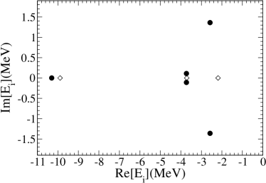
Figure 3: Like fig. 2 for the five pair energies in ²²C.

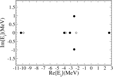
Figure 4: Like fig. 2 for the six pair energies in ²⁴C.

Table 2 also shows the ground state energy $E_{0}$ of the Carbon isotopes ¹⁴C to ²⁴C. Fig. 5 compares the calculated ground-state energy with the experimental one Audi et al. (2003). It is found that the exact solutions follow the overall trend, i.e. the binding energy decreases faster at the beginning of the chain and decelerates when it approaches the drip line. The agreement with data worsen as the number of neutrons increases. Even when the pairing interaction is a schematic one, and not realistic, this investigation suggests that the nucleus ²⁴C is unbound.

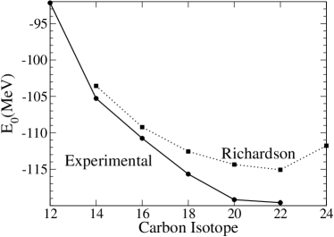
Figure 5: Carbon isotopes ground-state energy.

III.2.2 Carbon Isotopes Spectrum

It is worthwhile to compare the experimental spectrum with the exact solutions of the schematic pairing Hamiltonian corresponding to the cases of seniority-zero and seniority-two.

¹⁴C Spectrum: Table 3 gives the excitation spectrum (last column) with respect to the ground state configuration $(1)^{2}$. The seniority $\nu$, the pair energies and the number of pair $N_{\rm pair}=(A-12)-\nu$ ($A$ the mass number) are also given. Figure 6 compares the calculated levels from table 3 with that of the experimental one. The quantum number of the first excited state $1^{-}$ is correctly found with $1.5$ MeV less energy. The $0^{+}_{2}$ and $0^{+}_{3}$ excited states are underestimated with respect to the experimental one by $0.951$ MeV and $1.517$ MeV respectively. The state $3^{-}$ is found $1.37$ MeV below the experimental one. The splitting between the states $3^{-}$ and $0^{+}_{2}$ is well reproduced: $280$ keV versus the experimental $175$ keV but in inverse order. We missed the first $2^{+}$ state and found a $2^{+}$ at only $129$ keV from the second experimental $2^{+}$. The near degenerate experimental states $2^{+}$ and $4^{+}$ around $10$ MeV are well reproduced.

Table 3: Excited and pair energies of ¹⁴C. The energies are in MeV.

Config	$\nu$	State	$N_{\rm pair}$	$E_{p_{i}}$	$E$	$Ex$
$(1)^{2}$	0	$0^{+}$	1	$E_{p_{1}}=-11.398$	$-11.398$	$0$
$(1)(2)$	2	$0^{-},1^{-}$	0		$-6.803$	$4.594$
$(1)(3)$	2	$2^{-},3^{-}$	0		$-6.039$	$5.358$
$(2)^{2}$	0	$0^{+}$	1	$E_{p_{2}}=-5.760$	$-5.760$	$5.638$
$(3)^{2}$	0	$0^{+}$	1	$E_{p_{3}}=-3.168$	$-3.168$	$8.229$
$(2)(3)$	2	$2^{+}$	0		$-2.950$	$8.447$
$(3)(3)$	2	$2^{+},4^{+}$	0		$-1.093$	$10.304$

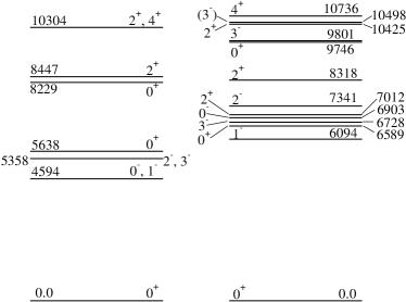
Figure 6: Exact low energy spectrum of ¹⁴C for seniority zero and two compared with experimental levels Audi et al. (2003). The energies are in keV.

¹⁶C Spectrum: Table 4 shows the pair energies and the excitation spectrum with respect to the ground state configuration $(1)^{2}(2)^{2}$. Fig. 7 compares the calculated versus the experimental spectrum of ¹⁶C. The first excited $2^{+}$ state does not appear in our spectrum. The first $0^{+}$ excited state is very well reproduce with a difference of only $21$ keV. We found a $2^{+}$ state at $3.274$ MeV which may correspond to the experimental $2$ state at $3.986$ MeV. The first $4^{+}$ excited state is found only $125$ keV below the experimental one. The experimental $(3^{-})$ is $406$ keV from the $3^{-}$ calculated state. In the exact spectrum appears a third $0^{+}$ state which does not appear in the experimental spectrum. Finally, the expaerimental $(4^{+})$ state is $938$ keV from the $4^{+}$ calculated one. Summing up what we found for the nucleus ¹⁶C, the first $0^{+}$, $4^{+}$ and $3^{-}$ are reasonable well described by the pairing interaction.

Table 4: Like table 3 for ¹⁶C.

Config	$\nu$	State	$N_{\rm pair}$	$E_{i}[MeV]$	$E[MeV]$	$Ex[MeV]$
$(1)^{2}(2)^{2}$	0	$0^{+}$	2	$E_{1}=-10.681$	$-17.051$	$0$
				$E_{2}=-6.370$
$(1)^{2}(3)^{2}$	0	$0^{+}$	2	$E_{1}=-10.823$	$-14.003$	$3.048$
				$E_{3}=-3.180$
$(1)^{2}(2)(3)$	2	$2^{+},3^{+}$	1	$E_{1}=-10.827$	$-13.777$	$3.274$
$(1)^{2}(3)(3)$	2	$2^{+},4^{+}$	1	$E_{1}=-10.848$	$-13.034$	$4.017$
$(2)^{2}(1)(3)$	2	$2^{-},3^{-}$	1	$E_{2}=-5.309$	$-11.348$	$5.703$
$(2)^{2}(3)^{2}$	0	$0^{+}$	2	$E_{2,3}=(-4.777,\pm 1.079)$	$-9.554$	$7.497$
$(2)^{2}(3)(3)$	2	$2^{+},4^{+}$	1	$E_{2}=-4.827$	$-7.013$	$10.038$

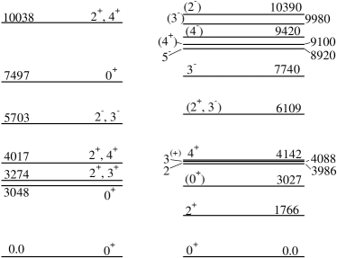
Figure 7: Like fig. 6 for ¹⁶C. The experimental levels above $6.11$ MeV are from Bohlen et al. (2003). The energies are in keV.

¹⁸C and ²⁰C Spectra: Tables 5 and 6 show the pair energies and the excitation spectrum with respect to the ground state configuration for the three and four pair systems ¹⁸C and ²⁰C respectively. Figure 8 shows the calculated exact eigenvalue of the pairing Hamiltonian for ¹⁸C and ²⁰C. Experimentally, only one excited state in ¹⁸C is known. It is a $(2^{+})$ state at $1620$ keV from the $(0^{+})$ ground state. Considering what we learn in the previous spectra one may place some confidence on the theoretical estimation for the levels $0^{+}_{2}$, $4^{+}_{1}$ and $3^{-}_{1}$.

Table 5: Like table 3 for ¹⁸C.

Config	$\nu$	State	$N_{\rm pair}$	$E_{i}[MeV]$	$E[MeV]$	$Ex[MeV]$
$(1)^{2}(2)^{2}(3)^{2}$	0	$0^{+}$	3	$E_{1}=-10.495$	$-20.394$	$0$
				$E_{2,3}=(-4.950;\pm 1.262)$
$(1)^{2}(2)^{2}(3)(3)$	2	$2^{+},4^{+}$	2	$E_{1}=-10.531$	$-17.525$	$2.869$
				$E_{2}=-4.809$
$(1)^{2}(3)^{2}(2)(3)$	2	$2^{+},3^{+}$	2	$E_{1}=-10.543$	$-17.203$	$3.191$
				$E_{3}=-3.710$
$(1)^{2}(3)^{4}$	0	$0^{+}$	3	$E_{1}=-10.549$	$-17.020$	$3.374$
				$E_{2,3}=(-3.236;\pm 0.474)$
$(1)^{2}(3)^{2}(3)(3)$	2	$2^{+},4^{+}$	2	$E_{1}=-10.573$	$-15.388$	$5.006$
				$E_{3}=-2.630$
$(2)^{2}(3)^{2}(1)(3)$	2	$2^{-},3^{-}$	2	$E_{2,3}=(-4.177;\pm 0.772)$	$-14.393$	$6.001$
$(3)^{4}(1)(2)$	2	$0^{-},1^{-}$	2	$E_{2,3}=(-3.576;\pm 0.981)$	$-13.955$	$6.439$
$(2)^{2}(3)^{4}$	0	$0^{+}$	3	$E_{2}=-4.405$	$-11.659$	$8.735$
				$E_{1,3}=(-3.627;\pm 1.433)$
$(2)^{2}(3)^{2}(3)(3)$	2	$2^{+},4^{+}$	2	$E_{2}=-4.008$	$-9.347$	$11.047$
				$E_{3}=-3.243$

Table 6: Like table 3 for ²⁰C.

Config	$\nu$	State	$N_{\rm pair}$	$E_{i}[MeV]$	$E[MeV]$	$Ex[MeV]$
$(1)^{2}(2)^{2}(3)^{4}$	0	$0^{+}$	4	$E_{1}=-10.379$	$-22.194$	$0$
				$E_{2}=-4.502$
				$E_{3,4}=(-3.667;\pm 1.546)$
$(1)^{2}(2)^{2}(3)^{2}(3)(3)$	2	$2^{+},4^{+}$	3	$E_{1}=-10.369$	$-19.813$	$2.381$
				$E_{2}=-3.993$
				$E_{3}=-3.238$
$(1)^{2}(3)^{4}(2)(3)$	2	$2^{+},3^{+}$	3	$E_{1}=-10.406$	$-19.047$	$3.147$
				$E_{3,4}=(-2.846;\pm 0.665)$
$(2)^{2}(3)^{4}(1)(3)$	2	$2^{-},3^{-}$	3	$E_{2}=-4.080$	$-15.969$	$6.225$
				$E_{3,4}=(-2.925;\pm 0.896)$
$(3)^{6}(1)(2)$	2	$0^{-},1^{-}$	3	$E_{4}=-3.167$	$-15.201$	$6.993$
				$E_{2,3}=(-2.615;\pm 1.113)$

Figure 8: Exact low energy spectra of ¹⁸C and ²⁰C for seniority zero and two. The energies are in keV.

III.3 Results: Complex Energy Representation

The first step in the determination of the complex representation is to find the resonant partial waves. This is done by evaluating the outgoing solutions (Gamow states) of the Schrodinger equation Gamow (1928); Berggren (1968) of the mean field Hamiltonian defined in Sec. III.1.1. Then, the half-life of the Gamow state is compared with the characteristic time of the system $\tau_{c}=5.953\times 10^{-23}$ sec (see Sec. II.6). Table 7 compares the characteristic time with the half-life of the states $\varepsilon_{0d_{3/2}}$ and $\varepsilon_{0f_{7/2}}$. The half-life of the state $0d_{3/2}$ is around nine times bigger than the characteristic time. The $0f_{7/2}$ state seems to be a wide resonance, but the comparison with the characteristic time shows that its half-life is a bit bigger than $\tau_{c}$.

Table 7: Comparison of the half-life versus the characteristic time (Sec. II.6).

state	$T_{1/2}$ [sec]	$T_{1/2}/\tau_{c}$
$0d_{3/2}$	$5.485\times 10^{-22}$	$9.21$
$0f_{7/2}$	$7.505\times 10^{-23}$	$1.26$

The effect of the resonant continuum was already investigated in ref. Hasegawa and Kaneko (2003). In order to investigate the effect of the non resonant continuum on the many-body correlations we compare in fig. 9 the ground state energy of the nucleus ²²C as a function of the pairing strength for three different model spaces: (i) Bound: $\{0p_{1/2},1s_{1/2},0d_{5/2}\}$, (ii) Resonant: $\{0p_{1/2},1s_{1/2},0d_{5/2},0d_{3/2},0f_{7/2}\}$, and (iii) Continuum (Secc. III.2). It is observed that the resonant and non resonant continuum states can be neglected as long as the pairing force is not very strong Hasegawa and Kaneko (2003). As the interaction increases the continuum starts to be important. The curve labeled as ”Continuum Representation” gives the ground state energy when the resonant and non resonant continuum is included in the representation through the CSPLD. The figure shows clearly the energy gain due to the inclusion of the continuum. The curve labeled as “Resonant Representation” gives the energy when only the resonant states are included in the representation. For very big strength the non resonant continuum becomes as important as the resonant continuum.

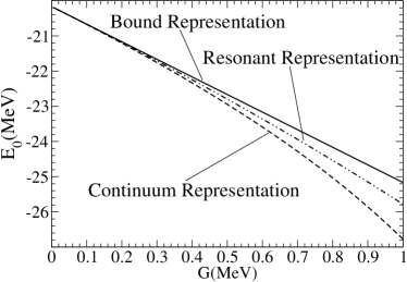
Figure 9: Ground state energy of ²²C versus pairing strength $G$ for three different model spaces.

Let us compare the evolution of the pair energies $E_{i}$ in the bound and the resonant representation versus the pairing strength. Figure 10 shows $E_{i}$ for $G$ from $G=1.0$ MeV to $G=0.005$ MeV in the nucleus ²²C . The continuum (dot) line corresponds to bound (resonant) representation. The deeper pair energy $E_{1}$ is little affected by the model space (one can not distinguish between the two curves). The other pairs are more affected for big value of the strength. The difference diminishes as the interaction decreases. The same effect was observed in the ground state energy (fig. 9). The pairs $E_{2}$ and $E_{3}$ are complex conjugate partners for $G\gtrsim 0.51$ MeV and they move at the same pace as $G$ changes. When they become real $E_{2}$ approaches to the uncorrelated pair energy $2\varepsilon_{2}$ while $E_{3}$ moves faster to the uncorrelated pair energy $2\varepsilon_{3}$. The pairs $E_{4}$ and $E_{5}$ remain complex conjugate for all no zero values of the strength.

Figure 10: Pair energies in the ground state ²²C versus pairing strength $G$ for $G=1.0$ MeV to $G=0.005$ MeV. The continuum line corresponds to the bound representation while the dot line corresponds to the resonant representation. The arrows point in the direction of decreasing $G$.

As a last application we will calculate the evolution of pair energies in the continuum, i.e. pair energies with positive real component. To this aim let us study the nucleus ²⁸C with eight pairs. Fig. 11 shows the evolution of the pairs for strength from $G=2.2$ MeV to $G=0.2$ MeV. The bound (negative real component) pairs $E_{1}$ to $E_{5}$ follow a trajectory similar to that in ²²C with the difference that the complex partners $E_{2}-E_{3}$ and $E_{4}-E_{5}$ are only approximately complex conjugate to each other. They become truly complex conjugate partners as the interaction approaches zero. On the other hand, the pairs in the continuum show a striking behavior. The typical movement to the right is not follow by all the positive energy pairs, i.e the continuum pairs may converge to its uncorrelated energy from right or left as $G$ decreases. Besides, the pairs seem to converge to the real part of the uncorrelated pair energy $lim_{G\rightarrow 0^{+}}E_{i}=2Re[\varepsilon_{i}]$ when $\varepsilon_{i}$ is a Gamow state.

Figure 11: Evolution of the pair energies in the ground state of ²⁸C as a function of the pairing strength $G$ from $G=2.2$ MeV to $G=0.2$ MeV. The arrows point in the direction of decreasing $G$.

IV Conclusion

The contribution of this paper to the exact solution of the pairing Hamiltonian is the inclusion of the resonant and non resonant continuum through the continuum single particle level density (CSPLD). The Gamow states, which appear in the complex energy representation, provide the main contribution from the continuum. It is worthwhile to point out that in the representation these states have exactly the same status as bound states. The difference is that the states in the continuum are no affected by blocking effects. The inclusion of the continuum has allowed us to study the unbound isotope ²⁴C and beyond. It was found that the continuum pairs (pair energies with positive real components) converge to the real part of the uncorrelated pair energy and they do not appear in complex conjugate partners. As a consequence the total energy may be complex. It was shown that from the exact solution of the pairing Hamiltonian the CSPLD can be used to investigate the effects of the resonant and non resonant continuum states upon the many-body pairing correlations.