Control of transport characteristics in two coupled Josephson junctions

Abstract

We report on a theoretical study of transport properties of two coupled Josephson junctions and compare two scenarios for controlling the current-voltage characteristics when the system is driven by an external biased DC current and unbiased AC current consisting of one harmonic. In the first scenario, only one junction is subjected to both DC and AC currents. In the second scenario the signal is split – one junction is subjected to the DC current while the other is subjected to the AC current. We study DC voltages across both junctions and find diversity of anomalous transport regimes for the first and second driving scenarios.

05.60.-k, 74.50.+r, 85.25.Cp 05.40.-a

1 Introduction

In symmetric devices, transport can be generated by nonequilibrium forces which can break space or time symmetry. In mechanical systems like movement of a Brownian particle in a spatially periodic and symmetric potential, the directed motion can be induced by an external static load forces or by unbiased multi-harmonic forces. Another class of systems with broken spatial symmetries is related to ratchet systems studied intensively during last twenty years [1]. In the paper, we study a relatively simple symmetric system which is constructed from the well-known physical elements: Josephson junctions. Their role in physics is invaluable and multifaceted, offering a rich spectrum of beneficial applications: from the definition of the voltage standard, through more practical devices as elements in high speed circuits [2], to the future applications in quantum computing devices [3]. We study two Josephson junctions coupled by an external resistance. The evolution of the system can manifest counterintuitive nature when we test its response to a constant external current: it can exhibit the negative resistance [4]. We can formulate the general question: how to manipulate the system by external drivings to get optimal and desired transport behaviour? To answer this question, we propose to manipulate the system by two combinations of external currents.

The paper is organized in the following way: In Sec. 2, we define the model and provide all necessary definitions and notation. Next, in Sec. 3, we study the response of the system in the case when external DC and AC currents are applied to one junction only. In Sec. 4, we analyze the case when the DC current is applied to the first junction and the AC current is applied to the second junction. In Sec. 5, comparison of transport characteristics for two driving scenarios is presented.

2 Model

From a more fundamental point of view, we consider a system which consists of two coupled (interacting) subsystems and we want to uncover its transport properties induced by coupling between two subsystems. As a particular example of the real physical structure, we study a Josephson junction device which consists of a coupled pair of resistively shunted Josephson junctions characterized by the critical Josephson supercurrents $(I_{c1},I_{c2})$, normal state resistances $(R_{1},R_{2})$ and phases $(\phi_{1},\phi_{2})$ [5]. A schematic circuit representing the model is shown in Fig. 1. The system is externally shunted by the resistance $R_{3}$ and driven by two current sources $I_{1}(t)$ and $I_{2}(t)$ acting on the first and second junctions, respectively.

Figure 1: The system of two coupled Josephson junctions shunted by an external resistance $R_{3}$ and driven by the external currents $I_{1}(t)$ and $I_{2}(t)$.

We also include into the model Johnson-Nyquist thermal noise sources $\xi_{1}(t),\xi_{2}(t)$ and $\xi_{3}(t)$ associated with the corresponding resistances $R_{1},R_{2}$ and $R_{3}$ according to the fluctuation–dissipation theorem. We assume the semiclassical and small junction regimes where the spatial dependence of characteristics can be neglected and photon-assisted tunnelling phenomena do not contribute to the general dynamics. It is the regime in which the so-called Stewart-McCumber model [6] holds true. The range of validity of this model is discussed in detail in the review paper [7].

The Kirchhoff current and voltage laws, and two Josephson relations allow for the full description of the phase dynamics of both junctions within assumed restrictions. The dimensional form of the equations of motion is presented in Ref. [8]. Therein, the dimensionless variables and parameters are defined, and the dimensionless form of dynamics is presented. Here, we recall only the dimensionless version of equations of motion for the phases $\phi_{1}=\phi_{1}(\tau)$ and $\phi_{2}=\phi_{2}(\tau)$, namely,

$$\dot{\phi}_{1}=I_{1}(\tau)-I_{c1}\sin\phi_{1}+\alpha[I_{2}(\tau)-I_{c2}\sin\phi_{2}]+\sqrt{D}\;\eta_{1}(\tau),$$

$$\dot{\phi}_{2}=\alpha\beta[I_{2}(\tau)-I_{c2}\sin\phi_{2}]+\alpha[I_{1}(\tau)-I_{c1}\sin\phi_{1}]+\sqrt{\alpha\beta D}\;\eta_{2}(\tau),$$ (1)

where the dot denotes a derivative with respect to dimensionless time $\tau$, which is defined by the dimensional time $t$ in the following way [9]

$$\tau=\frac{2eV_{0}}{\hbar}t,$$ (2)

where

$$V_{0}=I_{c}\frac{R_{1}(R_{2}+R_{3})}{R_{1}+R_{2}+R_{3}},\quad I_{c}=\frac{I_{c1}+I_{c2}}{2}$$ (3)

are the characteristic voltage and averaged critical supercurrent, respectively. All dimensionless currents in Eqs. (2) are in units of $I_{c}$. E.g., $I_{c1}\to I_{c1}/I_{c}$. The parameters

$$\alpha=\left(1+\frac{R_{3}}{R_{2}}\right)^{-1}\in[0,1],\quad\beta=1+\frac{R_{3}}{R_{1}}.$$ (4)

We assume that all resistors are at the same temperature $T$ and that the noise sources are modelled by independent $\delta$–correlated zero-mean Gaussian white noises $\xi_{i}(t)\ (i=1,2,3)$, i.e., $\left<\xi_{i}(t)\xi_{j}(s)\right>=\delta_{ij}\delta(t-s)$ for $i,j\in\{1,2,3\}$. The $\delta$–correlated zero-mean Gaussian white noises $\eta_{1}(t)$ and $\eta_{2}(t)$ which appear in Eqs. (2) are linear combinations of the original noises $\xi_{i}(t)$ and the resulting dimensionless noise strength reads $D=4ek_{B}T/\hbar I_{c}$.

Here we would like to stress out that the dimensional equations of motion for phases $\phi_{1}$ and $\phi_{2}$ are symmetrical with respect to the transformation $R_{1}\leftrightarrow R_{2}$. However, their dimensionless equivalents (2) are not symmetrical with respect to the change $R_{1}\leftrightarrow R_{2}$. It is because of: (i) the definition of the dimensionless time (2) which is extracted from the equation of motion for $\phi_{1}$ and, in consequence, (ii) the asymmetry of $V_{0}$ in Eq. (3) with respect to $R_{1}$ and $R_{2}$ .

Sometimes, it might be helpful to image the dynamics of two Josephson junctions described by Eqs. (2) as a motion of two interacting Brownian particles driven by external time-dependent forces. In this mechanical framework we have the following correspondence: $x_{1}=\phi_{1}$, $x_{2}=\phi_{2}$, where $x_{i}$ for $i=1,2$ stands for the coordinate of the first and second particles, respectively. The main transport characteristic of such a mechanical system are the long-time averaged velocities $v_{1}=\langle\dot{\phi_{1}}\rangle$ and $v_{2}=\langle\dot{\phi_{2}}\rangle$ of the first and second particles, respectively. In terms of the Josephson junction system it corresponds to the dimensionless long-time averaged voltages $v_{1}=\langle\dot{\phi_{1}}\rangle$ and $v_{2}=\langle\dot{\phi_{2}}\rangle$ across the first and second junctions, respectively (from the Josephson relation, the dimensional voltage $V=(\hbar/2e)d\phi/dt$ and therefore $d\phi/d\tau=V/V_{0}$). The junction resistance (or equivalently conductance) translates then into the particle mobility. The phase space of the deterministic system (2) is three-dimensional, namely $\{x_{1}=\phi_{1},x_{2}=\phi_{2},x_{3}=\omega t\}$. Note that it is a minimal dimension for the system to display chaotic evolution in continuous dynamical systems which may be a key feature for anomalous transport to arise [10, 11, 12, 13]. Other aspects of dynamics of two coupled Brownian particles has been studied in literature [14]. However, experimental realizations of such systems would be difficult to construct.

The considered system is characterized by four dimensionless material constants: $\{I_{c1},I_{c2},\alpha,\beta\}$ and by the dimensionless temperature $D$. Additionally, drivings $I_{1}(\tau)$ and $I_{2}(\tau)$ are also characterized by some parameters. In order to reduce a number of parameters of the model we consider a system of two identical junctions, i.e., $R_{1}=R_{2}$ and $I_{c1}=I_{c2}\equiv 1$. In such a case $\alpha\beta=1$ and Eqs. (2) takes the symmetric form

$$\dot{\phi}_{1}=I_{1}(\tau)-\sin\phi_{1}+\alpha[I_{2}(\tau)-\sin\phi_{2}]+\sqrt{D}\;\eta_{1}(\tau),$$

$$\dot{\phi}_{2}=I_{2}(\tau)-\sin\phi_{2}+\alpha[I_{1}(\tau)-\sin\phi_{1}]+\sqrt{D}\;\eta_{2}(\tau).$$ (5)

The parameter $\alpha$ plays the role of the coupling constant between two junctions and can be changed by variation of the external resistance $R_{3}$. The set of two differential equations is decoupled for $\alpha=0$ which results with two independent subsystems. It is the case when $R_{3}\to\infty$. Note that when $R_{3}=0$, the parameter $\alpha=1$ and the system is coupled.

3 The first scenario: DC and AC currents applied only to one junction

The external dimensionless currents $I_{1}(\tau)$ and $I_{2}(\tau)$ can be modelled in a various way. In experiments with Josephson junctions, ’the most popular’ three classes of currents have been applied: DC currents, AC currents consisting one harmonic and AC biharmonic currents:

$$I_{i}(\tau)=I_{i}+a_{i}\cos(\omega_{i}\tau)+b_{i}\cos(\Omega_{i}\tau+\theta_{i}),\quad i=1,2.$$ (6)

We start with the first scenario in which we apply the external current to the first junction only, namely,

$$I_{1}(\tau)=I_{1}+a_{1}\cos(\omega\tau),\quad I_{2}(\tau)=0.$$ (7)

In this special case Eqs. (2) take the form:

$$\dot{\phi}_{1} = I_{1}-\sin\phi_{1}-\alpha\sin\phi_{2}+a_{1}\cos(\omega\tau)+\sqrt{D}\;\eta_{1}(\tau),$$ (8)

$$\dot{\phi}_{2} = \alpha I_{1}-\sin\phi_{2}-\alpha\sin\phi_{1}+\alpha a_{1}\cos(\omega\tau)+\sqrt{D}\;\eta_{2}(\tau).$$ (9)

This case was considered in Ref. [15] in the context of indirect control of transport and absolute negative conductance induced by coupling between two junctions. Here, for the reader’s convenience, we recall the main transport characteristics of the system but just before we’ll do it let us clarify some technical issues.

The above set of equations cannot be handled by known analytical methods for solving ordinary differential equations. For this reason we have carried out extensive numerical simulations. We have used the stochastic version of Runge-Kutta algorithm of the $2^{nd}$ order with the time step of $10^{-3}\cdot(2\pi/\omega)$. The initial phases $\phi_{1}(0)$ and $\phi_{2}(0)$ have been randomly chosen from the interval $[0,2\pi]$. Averaging was performed over $10^{3}-10^{6}$ different realizations and over one period of the external driving $2\pi/\omega$. Numerical simulations have been carried out using CUDA environment on desktop computing processor NVIDIA GeForce GTX 285. This gave us possibility to speed up the numerical calculations up to few hundreds times more than on typical modern CPUs. Details on this very efficient method can be found in [16].

The voltage $v_{i}=v_{i}(I_{1}),i=1,2$, is typically a nonlinear and non-monotonic function of the DC current $I_{1}$. In the normal transport regime the nonlinear resistance or the static resistance $R_{i}=R_{i}(I_{1})=v_{i}(I_{1})/I_{1}$ (or equivalently conductance $C_{i}=1/R_{i}$) is positive at a fixed bias $I_{1}$. When the system response is opposite to the external driving, i.e., when $R_{i}<0$ we reveal the anomalous transport regime with absolute negative resistance (ANR) [11, 12] or nonlinear negative resistance (NNR) [13].

Now we would like to address some general comments about the long-time behaviour of the considered system (3). Let us consider the voltages $v_{1}=v_{1}(I_{1})$ and $v_{2}=v_{2}(I_{1})$ as functions of the DC bias. If we make the transformation $I_{1}\to-I_{1}$ to Eqs. (3), we note that $v_{1}(-I_{1})=-v_{1}(I_{1})$ and $v_{2}(-I_{1})=-v_{2}(I_{1})$ (because the functions $\sin\phi_{i}$ and $\cos(\omega\tau)$ are symmetric and noises $\eta_{i}(\tau)$ are also symmetric). From these relations it follows that $v_{1}(0)=-v_{1}(0)$, $v_{2}(0)=-v_{2}(0)$ and we deduce that $v_{1}(0)=0$ and $v_{2}(0)=0$ when the DC bias is zero, i.e., for $I_{1}=0$. From results of Ref. [15] it follows that for high frequency $(\omega>5)$, the long time averaged voltages $v_{i}$ are negligible small. It is because very fast positive and negative changes of the driving cannot induce transport. If the DC current is sufficiently large, it is rather obvious that voltages across both junctions has the same sign as the DC bias and depend (almost) linearly on the DC current. For the DC current $I_{1}>0$, one can identify three remarkable and distinct transport regimes:

• $v_{1}>0$ and $v_{2}>0$,

• $v_{1}>0$ and $v_{2}<0$,

• $v_{1}<0$ and $v_{2}<0$.

The regime (IV): $v_{1}<0$ and $v_{2}>0$ has not been detected.

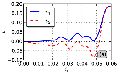
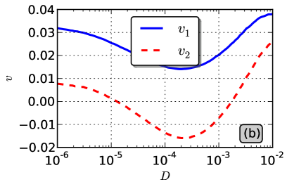
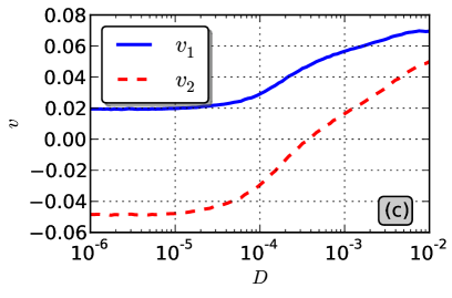
Figure 2: (color online). The first scenario: the long-time averaged voltages $v_{i}$ for $i=1,2$ of the first and second junction. Panel (a) illustrates the dependence on the DC current $I_{1}$ at the fixed temperature $D=2\cdot 10^{-5}$. In the panel (b) and (c) dependence on temperature $D$ is depicted for $I_{1}=0.025$ and $I_{1}=0.0455$, respectively. Other parameters read: coupling strength $\alpha=0.77$, amplitude $a_{1}=1.775$ and frequency $\omega=0.1875$ of the AC driving, $I_{2}=a_{2}=0$.

From the analysis reported in Ref. [15] it follows that the most interesting transport effects can take place in the regime of small $I_{1}$. Indeed, it has been found that for $I_{1}<0.1$ the absolute value of the long-time average voltage across both junctions takes its highest values for $\omega<1$. For stronger coupling, strips of non-zero average voltage begin to appear at progressively lower values of the amplitude $a_{1}$ of the AC driving. They are also visible for the average voltage of the first junction, which means that the strips represent the regimes in the parameter space where both junctions operate synchronously. It is illustrated in Fig. 2. In this regime of parameters, we can detect several interesting effects:

• the DC voltage $v_{1}$ is positive but the voltage $v_{2}$ exhibits ANR for $I_{1}\to 0$ and NNR for larger value of $I_{1}$.

• There are two different mechanisms generating negative resistance in the second junction:

  • In the case $I_{1}=0.025$, the negative resistance is induced by thermal fluctuations: for $D=0$ the voltage $v_{2}>0$ and when temperature increases $v_{2}$ becomes negative. There is a restricted interval of temperature where the voltage $v_{2}$ is negative.

  • In the case $I_{1}=0.0455$, the negative resistance is generated by the deterministic dynamics because in the deterministic limit (when $D=0$) the DC voltage $v_{2}<0$.

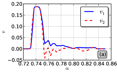
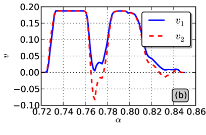
Figure 3: (color online). The first scenario: the long-time averaged voltages $v_{i}$ for $i=1,2$ across the first and second junction. The influence of the coupling parameter $\alpha$ on transport properties is depicted in the panels (a) and (b) for two fixed values of the DC current $I_{1}=0.025$ and $I_{1}=0.0455$, respectively. Other parameters are: temperature $D=2\cdot 10^{-5}$, amplitude $a_{1}=1.775$ and frequency $\omega=0.1875$ of the AC driving, $I_{2}=a_{2}=0$.

The anomalous transport effects like absolute negative resistance cannot occur in the decoupled system because in this case two decoupled and independent equations correspond to the overdamped dynamics for which the long-time average $v_{1}=\langle\dot{\phi}_{1}\rangle$ has the same sign as $I_{1}$ and $v_{2}=\langle\dot{\phi}_{2}\rangle=0$. Fig. 3 shows how the average voltage across the junctions depends on the coupling constant $\alpha$. One can note windows of $\alpha$ for which anomalous transport can be observed.

4 The second scenario: DC applied to the first junction and AC applied to the second junction

Nowadays technology allows experimentalists to apply driving to each of the junctions separately. In the following we would like to consider the scenario in which the DC current $I_{1}(\tau)=I_{1}$ is applied to the first junction and the AC current $I_{2}(\tau)=a_{2}\cos(\omega\tau)$ is applied to the second junction. The corresponding dynamics is described by the special case of Eqs. (2), namely,

$$\dot{\phi}_{1} = I_{1}-\sin\phi_{1}-\alpha\sin\phi_{2}+\alpha a_{2}\cos(\omega\tau)+\sqrt{D}\;\eta_{1}(\tau),$$ (10)

$$\dot{\phi}_{2} = \alpha I_{1}-\sin\phi_{2}-\alpha\sin\phi_{1}+a_{2}\cos(\omega\tau)+\sqrt{D}\;\eta_{2}(\tau).$$ (11)

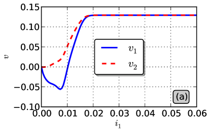
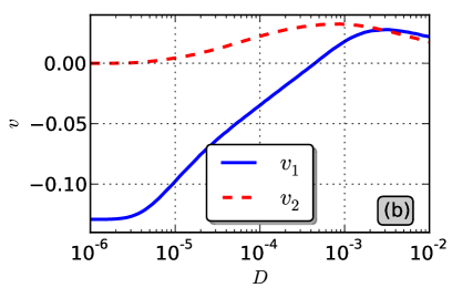
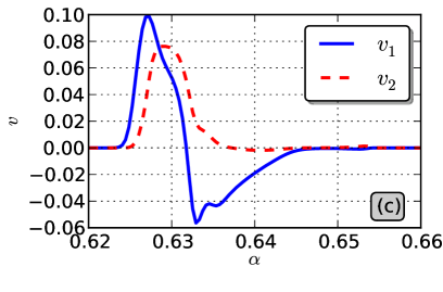
Figure 4: (color online). The second scenario: the long-time averaged voltages $v_{i}$ for $i=1,2$ across the first and second junction. Panel (a) illustrates the dependence on the DC bias $I_{1}$ at fixed value of amplitude $a_{2}=3.0023$, frequency of AC driving $\omega=0.1292$, the coupling strength $\alpha=0.6333$ and temperature $D=4.4\cdot 10^{-5}$. Panel (b) illustrates the temperature dependence for the DC current $I_{1}=0.0067$. Other parameters are the same as in panel (a). Panel (c) shows the role of coupling $\alpha$. Other parameters are the same as in panel (b).

This scenario leads to transport characteristics which in general are different than in the first scenario. In particular, for the DC current $I_{1}>0$, one can identify only two transport regimes where:

• $v_{1}>0$ and $v_{2}>0$,

• $v_{1}<0$ and $v_{2}>0$.

The regimes $\{v_{1}>0$ and $v_{2}<0\}$ and $\{v_{1}<0$ and $v_{2}<0\}$ have not been detected. This means that for this type of driving the transport properties are a little bit modest.

The regime (II) seems to be more interesting. In Fig. 4, we present the current-voltage characteristics in this regime. The unique feature is the emergence of the absolute negative resistance and the interval of $I_{1}$ where the averaged voltage across the first junction $v_{1}$ is negative. This is to be contrasted with the voltage $v_{2}$ which assumes only positive values. The regime of the nonlinear negative resistance is not found in this scenario. The most profound ANR effect occurs for the dc current $I_{1}=0.0067$. For this value, in panel (b) of Fig. 4, we show the voltage dependence on temperature $D$ of the system. A closer inspection of the panel (b) of Fig. 4 reveals a mechanism responsible for generating of anomalous transport. The negative resistance is solely induced by deterministic dynamics and even at zero temperature $D=0$ the resistance is negative. For this chaotic–assisted mechanism, temperature plays destructive role: if temperature increases the effect disappears and for temperature $D$ greater than $D=5\cdot 10^{-4}$ the averaged voltage $v_{1}$ is positive.

5 Comparison of transport characteristics for two scenarios

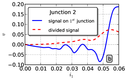
Figure 5: (color online). The second scenario: the long-time averaged voltage $v$ across the first (panel a) and the second (panel b) junction. The panels show the dependence on the dc bias $I_{1}$ at fixed temperature $D=2\cdot 10^{-5}$ for two different types of driving, ie. applied to only one junction ($a_{1}=1.775,a_{2}=0$, solid, blue line) and applied to both of them ($a_{1}=0,a_{2}=1.775$, dashed, red line). Other parameters are coupling strength $\alpha=0.77$, the frequency of the ac driving $\omega=0.1875$.

In the previous two sections we studied properties of the DC voltage across the first and second junctions driven by two different external currents. We presented the most interesting regimes where anomalous transport (i.e. negative resistance) can occur. There are three necessary ingredients for the anomalous transport to observe: DC bias, AC current (the nonequilibrium driving) and coupling. In this section, we compare transport properties in the same parameter domain but for two scenarios. In Fig. 5, the current-voltage curves are compared in the regime where the ANR and ANR is induced for the second junction in the first scenario and the DC voltage across the first junction is always positive, cf. Fig. 2(a). On the other hand, in the second scenario, the first junction exhibits very small absolute negative resistance while the DC voltage across the second junction is always positive. It means that the unbiased AC current can change the direction of transport (of course, the DC current can change it but it is rather trivial because the DC current is biased). In Fig. 6, we compare the above characteristics in dependence on temperature (the upper panels) and the coupling strength (the bottom panels) in the regime where anomalous transport is induced by thermal fluctuations.

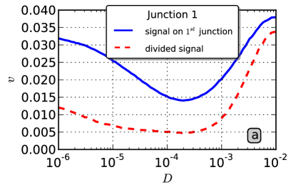
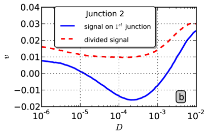
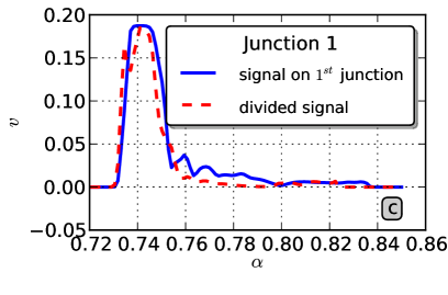
Figure 6: (color online). The long-time averaged voltage $v$ across the first (panels a and c) and second (panels b and d) junction. The upper panels show the dependence on temperature $D$ at fixed value of dc bias $I_{1}=0.025$ and the coupling strength $\alpha=0.77$ for two different types of driving, i.e. applied to only one junction ($a_{1}=1.775,a_{2}=0$, solid blue line) and applied to both of them ($a_{1}=0,a_{2}=1.775$, dashed red line). The bottom panels show the role of the coupling $\alpha$ for temperature $D=2\cdot 10^{-5}$. The frequency of the ac driving is $\omega=0.1875$.

For positive values of the DC current, one could expect four transport regimes:

• $v_{1}>0$ and $v_{2}>0$,

• $v_{1}>0$ and $v_{2}<0$,

• $v_{1}<0$ and $v_{2}<0$,

• $v_{1}<0$ and $v_{2}>0$.

In the first scenario, the regimes (I)-(III) can occur. In the second scenario, the regimes (I) and (IV) can occur. From this point of view, the first scenario seems to be more optimal: there are three regimes. From the symmetry of the system it follows that the regime (IV) could be obtained by applying the same driving to the second junction only.

In summary, we studied transport properties of two coupled Josephson junctions and compared two scenarios for controlling the current-voltage characteristics when the system is driven by an external biased DC current and unbiased AC current consisting of one harmonic. We uncovered a reach diversity of anomalous transport regimes for the first and second driving scenarios.

References

- [1] P. Hänggi and F. Marchesoni, Rev. Mod. Phys. 81, 387 (2009).
- [2] A. Barone and G. Paternò, Physics and Application of the Josephson Effect, (New York: Wiley) (1982).
-
[3]
Y. Makhlin, G. Schön, A. Shnirman, Rev. Mod. Phys. 73, 357 (2001);
M. Mariantoni et. al., Nature Physics 7, 287 (2011). - [4] R. A. Höpfel et al., Phys. Rev. Lett. 56, 2736 (1986); B. J. Keay et al., Phys. Rev. Lett. 75, 4102 (1995); S. Zeuner et al., Phys. Rev. B 53, R1717 (1996); E. H. Cannon et al., Phys. Rev. Lett. 85, 1302 (2000); H. S. J. van der Zant et al., Phys. Rev. Lett. 87, 126401 (2001); I. I. Kaya et al., Phys Rev. Lett. 98, 186801 (2007); X. B. Xu et al., Phys. Rev. B 75, 224507 (2007); J. Nagel et al., Phys. Rev. Lett. 100, 217001 (2008).
- [5] M. A. H. Nerenberg, J. A. Blackburn and S. Vik, Phys. Rev. B 30, 5084 (1984); J. Bindslev Hansen and P. E. Lindelof, Rev. Mod. Phys. 56, 431 (1984).
- [6] W. C. Stewart, Appl. Phys. Lett. 12, 277 (1968); D. E. McCumber, J. Appl. Phys. 39, 3113 (1968).
- [7] R. L. Kautz, Rep. Prog. Phys. 59, (1996).
- [8] L. Machura, J. Spiechowicz, M. Kostur, J. Łuczka, to appear in J. Phys. Condens. Matter, arXiv:1110.5287 (2012).
- [9] M. A. H. Nerenberg, J. A. Blackburn and D. W. Jillie, Phys. Rev. B 21, 118 (1980).
- [10] M. Kostur, L. Machura, P.Hänggi, J. Łuczka and P.Talkner, Physica A 371, 20 (2006).
- [11] L. Machura, M. Kostur, P. Talkner, J. Łuczka, P. Hänggi, Phys. Rev. Lett. 98, 040601 (2007).
- [12] D. Speer, R. Eichhorn, and P. Reimann, Europhys. Lett. 79, 10005 (2007); Phys. Rev. E 76, 051110 (2007).
-
[13]
L. Machura, M. Kostur, P. Talkner, P. Hänggi and J. Łuczka, Phys. Rev. E 42, 590 (2010);
M. Kostur, L. Machura, P. Talkner, P. Hänggi and J. Łuczka, Phys. Rev. B 77, 104509 (2008);
M. Kostur, L. Machura, J. Łuczka, P. Talkner and P. Hänggi, Acta Physica Polonica B 39, 1115 (2008). - [14] D. Speer, R. Eichhorn, and P. Reimann, Phys. Rev. Lett. 102, 124101 (2009); U. E. Vincent, A. Kenfack, D. V. Senthilkumar, D. Mayer, and J. Kurths, Phys. Rev. E 824, 046208 (2010); C. Mulhern and D. Hennig, Phys. Rev. E 84, 036202 (2011).
- [15] M. Januszewski and J. Łuczka, Phys. Rev. E 83, 051117 (2011).
- [16] M. Januszewski and M. Kostur, Comput. Phys. Commun. 181, 183 (2010).