Tuning the disorder in superglasses

Abstract

We study the interplay of superfluidity, glassy and magnetic orders in the XXZ model with random Ising interactions on a three dimensional cubic lattice. In the classical limit, this model reduces to a $\pm J$ Edwards-Anderson Ising model with concentration $p$ of ferromagnetic bonds, which hosts a glassy-ferromagnetic transition at a critical concentration $p_{c}^{\rm cl}\sim 0.77$. Our quantum Monte Carlo simulation results show that quantum fluctuations stabilize the coexistence of superfluidity and glassy order ( “superglass”), and shift the (super)glassy-ferromagnetic transition to $p_{c}>p_{c}^{\rm cl}$. In contrast, antiferromagnetic order coexists with superfluidity to form a supersolid, and the transition to the glassy phase occurs at a higher $p$.

Introduction–

Spin glasses are frustrated magnetic systems with quenched disorder, hosting glassy phases with extremely slow dynamicsBinder and Young (1986). Traditionally, the simplest model that exhibits spin glass (SG) behavior is the $\pm J$ Ising model, or Edwards-Anderson (EA) modelEdwards and Anderson (1975), in which Ising spins interact via randomly distributed nearest-neighbor (NN) ferromagnetic (FM) and antiferromagnetic (AFM) bonds with probability $p$ and $1-p$ respectively. This model has been studied extensively with Monte Carlo simulations and exhibits a finite temperature glass transition in three dimensions (3D) Kawashima and Young (1996); Ballesteros et al. (2000). It has been shown that this model has a second order transition from a SG to a FM (AFM) phase at a critical concentration $p_{c}=p_{c}^{\rm cl}\sim 0.77\,(p_{c}=1-p_{c}^{\rm cl}\sim 0.23)$ as one increases (decreases) the fraction of FM bonds, and there exists reentrance of the spin glass phase in the temperature-disorder phase diagramHartmann (1999); Hasenbusch et al. (2008); Ceccarelli et al. (2011). One natural question to ask is how the transition can be changed by quantum fluctuations Markland et al. (2011); Tam et al. (2010); Yu and Müller (2012). In particular, understanding the behavior of granular superfluidity in a frozen amorphous structure may give us hints on the microscopic mechanism of the formation of supersolids (SS) Kim and Chan (2004a); *Kim:2004fk.

The observation of supersolidity in solid Helium 4 (He⁴) Kim and Chan (2004a); *Kim:2004fk has spurred immense interests on the connection between superfluidity and disorder in bosonic systems. Strong experimental evidence suggest that disorder may play a role in how the supersolid formsRittner and Reppy (2007); *Rittner:2006uq. A recent experiment observed ultraslow dynamics in solid He⁴Hunt et al. (2009), suggesting a glassy type of supersolid, or a “superglass” (SuG)  Biroli et al. (2008); Wu and Phillips (2008); Tam et al. (2010); Yu and Müller (2012). Quantum Monte Carlo (QMC) studies on the extended hardcore Bose-Hubbard model with random frustrating interactions on a 3D cubic lattice indicate that glassiness can coexist with superfluidity, and quantum fluctuations and random frustration are both crucial in stabilizing the superglass stateTam et al. (2010).

While the phase transitions into superfluidity or quantum solid/glassy states have been studied in some detail, the nature of the various transitions into a SS/SuG are yet left unexplored. In this Letter, we study the XXZ model with random Ising interactions, which maps to an extended hardcore Bose-Hubbard model with random frustrating interactions, in order to characterize transitions by tuning the amount of disorder present in the interactions. We demonstrate that the presence of quantum exchange terms greatly increases the temperature dependence of the SuG-FM transition by pushing the low temperature phase boundary to a higher critical concentration than $p_{c}^{\rm cl}$. The SuG-SS phase boundary is also drawn to a higher critical concentration, and an asymmetry for SuG-SS and SuG-FM transitions arises.

Model–

The Hamiltonian for hardcore boson with a random NN interaction is

$${\mathcal{H}}=-\sum_{\langle i,j\rangle}V_{ij}(n_{i}-1/2)(n_{j}-1/2)-t\sum_{\langle i,j\rangle}(b_{i}^{\dagger}b_{j}+b_{i}b_{j}^{\dagger}),$$ (1)

where $\langle i,j\rangle$ indicates the NN lattice sites. $n_{i}$ is the number operator for hard-core bosons at lattice site $i$, $t$ is the hopping parameter and $V_{ij}$ are interactions with a bimodal distribution given as

$$p(V_{ij})=p\delta(V_{ij}-V)+(1-p)\delta(V_{ij}+V).$$ (2)

By a transformation of the bosonic operators to spin-1/2 operators: $S^{z}_{i}=n_{i}-1/2,S_{i}^{-}=b_{i}$, and $S_{i}^{+}=b^{\dagger}_{i}$, this model can be readily mapped into the standard XXZ model:

$${\mathcal{H}}=-\sum_{\langle i,j\rangle}J_{z}S_{i}^{z}S_{j}^{z}-\frac{1}{2}J_{xy}\sum_{\langle i,j\rangle}(S_{i}^{-}S_{j}^{+}+S_{i}^{+}S_{j}^{-}),$$ (3)

where $J_{xy}=2t$ and $J_{z}=V_{ij}$. This model reduces to the classical EA model if $J_{xy}=0$. The FM and AFM phases in the spin model correspond to quantum solid phases with $(0,0,0)$ and $(\pi,\pi,\pi)$ ordering vectors, respectively. In the following, we will use the spin language for simplicity.

There exist both diagonal and off-diagonal long-range orders in this model. Possible diagonal long-range orders are FM, AFM and SG, with corresponding order parameters: magnetization $m=\frac{1}{N}\sum_{i}S_{i}^{z}$ (FM), staggered magnetization $m_{s}=\frac{1}{N}\sum_{i}(-1)^{i}S_{i}^{z}$ (AFM), and the Edwards-Anderson order parameter (SG), defined as

$$q_{\rm EA}=\frac{1}{N}\left[{\sum_{i}\langle S_{i}^{z}\rangle^{2}}\right]_{\rm av},$$ (4)

where $\langle\cdots\rangle$ denotes a thermal average and $[\cdots]_{\rm av}$ an average over disorder realizations. As the EA order parameter will also capture FM and AFM ordering, one must look for a non-zero $q_{\rm EA}$ while the other order parameters remain zero in order to identify an SG phase.

To determine the phase transition point, we look at the Binder cumulants Binder (1981) for the order parameter, which should cross at the transition point for different system sizes. However, the existence of corrections to scaling cause pairs of small sizes to intersect away from the true critical point. To improve the accuracy of the measurement, we look at the series of intersection points created by successive pairs of sizes $L$ and $L+1$ which should converge to the exact value as a power law with the exponent determined by the leading correction to scaling. To get statistical estimates of these crossing points, we perform a bootstrap resampling on the raw data ($N_{\text{boot}}=100$), fitting a 2nd-order polynomial to each size, and calculating the resulting intersection. The Binder cumulants of the magnetization and staggered magnetization are

$$g_{\rm m}=\frac{1}{2}\left(3-\frac{\left[\langle m^{4}\rangle\right]_{\rm av}}{\left[\langle m^{2}\rangle\right]_{\rm av}^{2}}\right);\quad g_{\rm sm}=\frac{1}{2}\left(3-\frac{\left[\langle m_{s}^{4}\rangle\right]_{\rm av}}{\left[\langle m_{s}^{2}\rangle\right]_{\rm av}^{2}}\right)$$ (5)

which approach one in the FM/AFM phase and goes to zero otherwise. We measure the superfluid density through winding number fluctuationsPollock and Ceperley (1987),

$$\rho_{s}=\frac{1}{3\beta Nt}\left[\sum_{k=x,y,z}\langle W_{k}^{2}\rangle\right]_{\rm av},$$ (6)

where $W_{k}$ is the winding number along the $k$ direction. In our simulation, we identify the SS phase by the coexistence of AFM and SF orders, and the SuG phase by the coexistence of SG and SF orders.

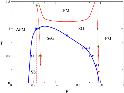
Figure 1: (Color online) $T$ vs $p$ phase diagram. The dashed lines indicate the position of the classical transitions SG-(A)FM, and the solid lines with arrows show the trend of the phase boundary shifts we find in the quantum model. The blue circles are our estimates for the superfluid transition, with the approximate phase boundary drawn as the blue arc. Lastly, the red arc denotes the PM-SG phase boundary.

Method–

We use the Worm Algorithm QMC Prokof’ev et al. (1998a); *Prokofev:1998vn to study this model, as well as the Stochastic Series Expansion (SSE) Sandvik (1999) with the parallel tempering Hukushima and Nemoto (1996); *Melko:2007fk near the FM boundary to access low temperaturesSM . We simulate many different realizations of the disorder–sets of interactions $V_{ij}$–for a given parameter set. In the following, we choose $V/t=4$ in order to maximize the extent of the superglass phase at $p=0.5$Tam et al. (2010). Each realization is simulated independently and equilibrium is determined by reaching measurements that stabilize within our error bars. Table  1 contains the details of our simulation parameters. For our worm algorithm implementation a Monte Carlo (MC) step is defined as $N_{\rm sites}=L^{3}$ completed worm loop updates, while for SSE we define it the same as Ref. Sandvik (1999) with the addition of one replica exchange sweep. Equilibration times vary across phases: worm update loops tend to be long while in SF phases, and under increasing ferromagnetic order the worms have a low probability of hopping producing short loops. This effect is significantly reduced in our SSE implementations since each MC step has an adaptively determined number of operator loop updates.

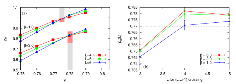
Figure 2: (Color online) (a) Finite size scaling of $g_{m}$ at $\beta=1$ and 3 to determine the SG-FM transition. Data for $\beta=1$ are shifted vertically for clarity. Shaded areas indicate the crossing for different sizes. Dotted line shows the position of the zero-temperature classical transition ($p_{c}^{\text{cl}}$). Our $p_{c}$ estimates show stronger reentrance. (b) Results of bootstrap estimates for the crossing points for adjacent sizes. Dotted line shows the position of the zero-temperature classical transition. Deviation from the classical transition point is clearly seen in the large size data points at $\beta=2$ and 3.

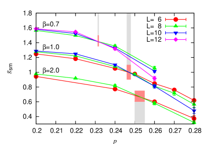
Figure 3: (Color online) Finite size scaling of the staggered magnetization cumulant $g_{sm}$. Data for $\beta=1$ and $\beta=0.7$ are shifted vertically for clarity. Results at $\beta=0.7$ are in line with classical behavior while $\beta=1,2$ suggest the SuG-SS transition has been drawn into the classical SG region.

Table 1: Parameters of the simulations

	$\beta$	$L$	$p$ range	$\sim N_{\text{samp}}$	$\sim N_{\text{sweep}}$
	0.70	6	0.20 - 0.26	600	8000
	0.70	8	0.20 - 0.26	400	16000
	0.70	10	0.20 - 0.26	500	64000
	0.70	12	0.20 - 0.26	250	128000
	1.00	3	0.70 - 0.80	2000	4000
	1.00	4	0.75 - 0.78	2000	16000
	1.00	5	0.75 - 0.78	800	128000
	1.00	6	0.75 - 0.78	150	256000
	1.00	6	0.12 - 0.28	1000	16000
	1.00	8	0.12 - 0.28	400	16000
	1.00	10	0.12 - 0.28	400	64000
	2.00	6	0.20 - 0.28	500	8000
	2.00	8	0.20 - 0.28	500	128000
	SSE	3	0.75 - 0.79	4700	16000
	SSE	4	0.75 - 0.79	4000	16000
	SSE	5	0.75 - 0.79	4000	16000
	SSE	6	0.75 - 0.79	4000	32000

Results–

Figure 1 summarizes our QMC results in a temperature-disorder ($T$-$p$) phase diagram. At high temperatures, we expect the model behaves classically, and is described by the 3D EA model. The classical phase diagram is symmetric about $p=0.5$ if one identifies the FM with the AFM regime. The classical 3D EA model undergoes a $T=0$ SG-FM transition at $p_{c}^{\rm cl}\sim 0.770$, and shows slight reentrant behavior at finite $T$ (red dashed lines). It is suggested that the finite-temperature SG-FM transition belongs to a new universality class with critical exponents $\nu=0.96(2)$ and $\eta=-0.39(2)$ Ceccarelli et al. (2011). The SG-FM, PM-SG and PM-FM transition lines meet at a multi-critical point $p=p^{*}$ (not shown), which sits on the Nishimori lineNishimori (1981); Ceccarelli et al. (2011), and the PM-SG transition for $1-p^{*}<p<p^{*}$ belongs to the Ising spin glass (ISG) universality classHasenbusch et al. (2007).

Entering the quantum regime, the SG-FM transition appears to become more temperature dependent and deviate from the classical behavior. Likely this is due to the encroaching superfluid order and subsequent competition. Meanwhile, the AFM state allows for superfluidity, creating a region of supersolidity within the arm of the superfluid transition line, which may be why the AFM state is more stable in the quantum model. Furthermore, the SuG-SS line pushes deeper into the SG phase, suggesting interesting correlation between the AFM and SF orders.

The results for our analysis of the magnetic ordering are presented in Fig. 2. Already at $\beta=1$ we see evidence for a shift in the phase boundary. By $\beta=3$ in Fig. 2 $(a)$, it is clear there would not be a transition for $p<0.78$, given the position of the data crossings as shown. This is markedly different than the classical results. The classical transition line $p_{c}^{\rm cl}$ as a function of $\beta$ is only weakly temperature dependent, shifting less than a percent between the multicritical point and zero temperatureCeccarelli et al. (2011). Here, that shift is at least 4 times as large. We have studied the superfluid transition as well for these parameters, and our estimates (see Fig. 1) are only rough due to the non-trivial nature of the superfluid scaling form. For a 3D XY model, one expects $\rho_{s}\sim~{}1/L^{\alpha}$ with $\alpha=1$ away from quantum criticality. However, we find $\alpha>1$ as the model enters the glass phase with, for example, $\alpha\approx 1.4-1.8$ for the transition at $p=0.5$ Larson and Kao (2012).

The specific mechanism behind the increased temperature dependence of the SuG-FM transition should be rooted in how superfluidity favors the spin glass phase over the ferromagnetic phase. One can imagine that clusters of FM-ordered spins are suppressed as the system can gain kinetic energy by destroying local ferromagnetic order and allowing particles to hop. On the other hand, glassy clusters more readily allow superfluid fluctuations amongst them, perhaps following lines of sites that are weakly constrained due to frustration. Thus a broader spin glass (thus superglass) phase is stabilized and the transition line is moved into the FM phase.

Figure 4: A typical 2D snapshot near the SuG-SS line. The hop move indicated is energetically neutral with respect to the bonds and destroys the local AFM order. However, the new state allows fewer fluctuations so is not favored with respect to entropy.

We also looked at the behavior on the other side, $p<0.5$, which is different due to the asymmetry of the ground state against quantum fluctuations. Notably, we find superfluid transitions at higher temperatures: $\beta_{c}(1-p)<\beta_{c}(p)$. Figure 3 shows data for the Binder cumulant using the staggered magnetization, $g_{sm}$ at $\beta=1$ and $2$. The staggered magnetization data suffer from larger FSE and subsequently require larger system sizes to achieve comparable precision, restricting the current study from exploring lower temperatures.

The position of the crossing at $\beta=1$ lies around $p_{c}\sim 0.25$ indicating that the SuG-SS line is noticeably shifted from classical behavior. The data at lower $T$ are less conclusive due to larger sizes being out of reach at present, but suggest an even larger shift. Above the SF transition at $\beta=0.7(T=1.43)$, the AFM-SG transition agrees with the classical transition point $p=1-p_{c}^{\rm cl}=0.23$. Thus, the stronger the quantum mechanical nature becomes–the deeper into the superfluid behavior we go–the stronger the AFM order appears. This is at first counterintuitive, but we can provide a simple, consistent picture for both this and the SuG-FM behavior. When an FM bond is satisfied, i.e. two neighboring sites are in the same state, this forbids hopping along that bond. Conversely, when an AFM bond is satisfied, the two sites are in an opposite state and will allow the system to gain kinetic energy through hops. As this is energetically favorable, we can consider the AFM bonds to have a larger effective bond strength. Consequently, the fraction of frustrating FM bonds it would require to destroy the AFM order should rise, and we see the present shift in phase boundary.

Speaking more generally, we can consider the change in the entropy of the system, with respect to quantum fluctuations, when moving towards higher AFM or FM order. Under pure FM order no hopping is allowed, while under pure AFM order each site has the ability to engage in virtual hopping. For the illustration purpose, Fig. 4 shows a typical local 2D snapshot of a system with AFM order being frustrated by FM bonds. The indicated move would go against three NN bonds while satisfying three others, making the diagonal component energetically neutral, and this would turn the local AFM order into FM order. However, after this move the system is now considerably more constrained regarding the number of hoppings available. Originally, the two interior sites could be involved with seven different hop moves, but these sites now have a single move: to return back to the original state. In this way, the AFM state is favored as it allows for more gain in kinetic energy.

Summary–

We have presented our QMC results of a model exhibiting a superglass phase in order to study the phase transitions achieved by directly tuning the level of disorder present. These results indicate that the addition of the exchange terms act to stabilize the classical spin glass phase against the formation of ferromagnetic clusters which impede hopping. In addition, the favoring of AFM bonds to FM bonds leads to a shift in the SuG-SS phase boundary. An interesting issue not addressed here is whether there is always a SG phase between the FM and SuG phases. Recent workPollet et al. (2009) on disordered Bose systems suggests that this may be true. Unfortunately, our current precision is not high enough to be conclusive. Future work is required to clarify this issue.

I Supplementary Material

Figure 5 shows the equilibration data of the magnetic Binder cumulant, using the stochastic series expansion (SSE) quantum Monte Carlo with parallel tempering (PT), near the ferromagnetic transition for $L=6$. Each data point is obtained by first equilibrating for a given number of sweeps ($N_{\rm sw})$, and the perform measurements for the same number of sweeps. For example, the point at $N_{\text{sw}}=2^{10}$ will have1024 sweeps for equilibration and then 1024 sweeps of measurement. In addition, averaging over different disorder realizations is carried out. It is clear that the simulations are well-equilibrated in the doping range of interests, $p=0.75-0.79$, and at all temperatures $T=0.3333,0.5000,1.0000$. Smaller sizes are all strongly equilibrated.

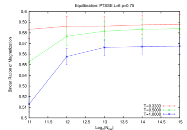
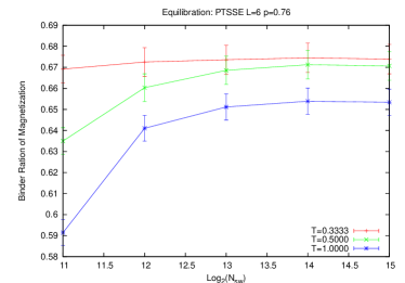
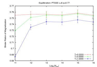
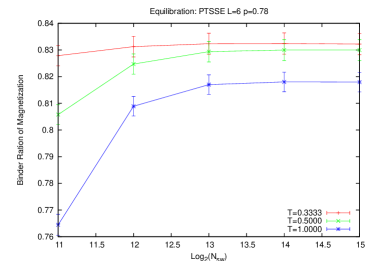
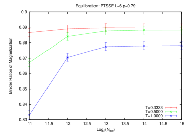
Figure 5: (Color online) Equilibration data for the SSE at the largest system size $(L=6)$ for $p=0.75-0.79$. Smaller sizes are all more strongly equilibrated.

References

- Binder and Young (1986) K. Binder and A. P. Young, Rev. Mod. Phys. 58, 801 (1986).
- Edwards and Anderson (1975) S. F. Edwards and P. W. Anderson, J. Phys. F: Met. Phys. 5, 965 (1975).
- Kawashima and Young (1996) N. Kawashima and A. P. Young, Phys. Rev. B 53, R484 (1996).
- Ballesteros et al. (2000) H. G. Ballesteros, A. Cruz, L. A. Fernández, V. Martín-Mayor, J. Pech, J. J. Ruiz-Lorenzo, A. Tarancón, P. Téllez, C. L. Ullod, and C. Ungil, Phys. Rev. B 62, 14237 (2000).
- Hartmann (1999) A. K. Hartmann, Phys. Rev. B 59, 3617 (1999).
- Hasenbusch et al. (2008) M. Hasenbusch, A. Pelissetto, and E. Vicari, Phys. Rev. B 78, 214205 (2008).
- Ceccarelli et al. (2011) G. Ceccarelli, A. Pelissetto, and E. Vicari, Phys. Rev. B 84, 134202 (2011).
- Markland et al. (2011) T. E. Markland, J. A. Morrone, B. J. Berne, K. Miyazaki, E. Rabani, and D. R. Reichman, Nat Phys 7, 134 (2011).
- Tam et al. (2010) K.-M. Tam et al., Phys. Rev. Lett. 104, 215301 (2010).
- Yu and Müller (2012) X. Yu and M. Müller, Phys. Rev. B 85, 104205 (2012).
- Kim and Chan (2004a) E. Kim and M. H. W. Chan, Nature 427, 225 (2004a).
- Kim and Chan (2004b) E. Kim and M. H. W. Chan, Science 305, 1941 (2004b).
- Rittner and Reppy (2007) A. S. C. Rittner and J. D. Reppy, Phys. Rev. Lett. 98, 175302 (2007).
- Rittner and Reppy (2006) A. S. C. Rittner and J. D. Reppy, Phys. Rev. Lett. 97, 165301 (2006).
- Hunt et al. (2009) B. Hunt, E. Pratee, V. Gadagkar, M. Yamashita, A. Balatsky, and J. C. Davis, Science 324, 632 (2009).
- Biroli et al. (2008) G. Biroli, C. Chamon, and F. Zamponi, Phys. Rev. B 78, 224306 (2008).
- Wu and Phillips (2008) J. Wu and P. Phillips, Phys. Rev. B 78, 014515 (2008).
- Binder (1981) K. Binder, Z. Phys. B 43, 119 (1981).
- Pollock and Ceperley (1987) E. L. Pollock and D. M. Ceperley, Phys. Rev. B 36, 8343 (1987).
- Prokof’ev et al. (1998a) N. Prokof’ev, B. Svistunov, and I. Tupitsyn, Physics Letters A 238, 253 (1998a).
- Prokof’ev et al. (1998b) N. Prokof’ev, B. Svistunov, and I. Tupitsyn, Journal of Experimental and Theoretical Physics 87, 310 (1998b), 10.1134/1.558661.
- Sandvik (1999) A. W. Sandvik, Phys. Rev. B 59, R14157 (1999).
- Hukushima and Nemoto (1996) K. Hukushima and K. Nemoto, J. Phys. Soc. Jpn. 65, 1604 (1996).
- Melko (2007) R. G. Melko, Journal of Physics: Condensed Matter 19, 145203 (2007).
- (25) See Supplemental Material at [URL will be inserted by publisher] for the equilibration data near the FM phase boundary.
- Nishimori (1981) H. Nishimori, Prog. Theor. Phys. 66, 1169 (1981).
- Hasenbusch et al. (2007) M. Hasenbusch, F. P. Toldin, A. Pelissetto, and E. Vicari, Phys. Rev. B 76, 094402 (2007).
- Larson and Kao (2012) D. A. Larson and Y.-J. Kao, Unpublished (2012).
- Pollet et al. (2009) L. Pollet, N. V. Prokof’ev, B. V. Svistunov, and M. Troyer, Phys. Rev. Lett. 103, 140402 (2009).