The local geometry of finite mixtures

Abstract.

We establish that for $q\geq 1$, the class of convex combinations of $q$ translates of a smooth probability density has local doubling dimension proportional to $q$. The key difficulty in the proof is to control the local geometric structure of mixture classes. Our local geometry theorem yields a bound on the (bracketing) metric entropy of a class of normalized densities, from which a local entropy bound is deduced by a general slicing procedure.

1. Introduction

Let $(X,d)$ be a metric space, and consider a subset $T=\{t_{\xi}:\xi\in\Xi\}$ of $X$ that is parametrized by a bounded subset $\Xi$ of $\mathbb{R}^{d}$. Roughly speaking, we are interested in the following question: can $T$ be viewed as a finite-dimensional subset of $X$? It is certainly tempting to think so, as the parameter set $\Xi$ is finite-dimensional. This idea is easily made precise if the induced metric $d_{T}(\xi,\xi^{\prime})=d(t_{\xi},t_{\xi^{\prime}})$ on $\Xi$ is comparable to a norm on $\mathbb{R}^{d}$, so that $T$ inherits the Euclidean geometry. However, there are natural examples whose geometry is highly non-Euclidean, so that the conclusion is far from obvious. The aim of this paper is to investigate in detail such a problem that arises from applications in statistics.

To set the stage for the problem that we will consider, let us recall some metric notions of dimension. For a subset $T$ of a metric space $(X,d)$, the covering number $N(T,\varepsilon)$ is the smallest cardinality of a covering of $T$ by $\varepsilon$-balls [15]:

$$N(T,\varepsilon)=\inf\bigg{\{}n:\exists~{}x_{i}\in X,~{}i=1,\ldots,n\mbox{ s.t.\ }T\subseteq\bigcup_{i=1}^{n}B(x_{i},\varepsilon)\bigg{\}},$$

where $B(x,\varepsilon)=\{x^{\prime}\in X:d(x,x^{\prime})\leq\varepsilon\}$. The covering number, or equivalently the metric entropy $\log N(T,\varepsilon)$, quantifies the capacity of the set $T$, and its scaling in $\varepsilon$ is closely connected to dimension. Indeed, let $|\cdot|$ be a norm on $\mathbb{R}^{d}$, so that $(\mathbb{R}^{d},|\cdot|)$ is a finite-dimensional Banach space. A standard estimate [17, Lemma 4.14] gives

$$N(B(t,\delta),\varepsilon)\leq\bigg{(}\frac{3\delta}{\varepsilon}\bigg{)}^{d}$$

for any $\varepsilon\leq\delta$, where $B(t,\delta)=\{x\in\mathbb{R}^{d}:|x-t|\leq\delta\}$. This estimate has two trivial consequences: first, for any bounded $T\subset(\mathbb{R}^{d},|\cdot|)$, there is a constant $C_{1}$ so that

(1.1) $$N(T,\varepsilon)\leq\bigg{(}\frac{C_{1}}{\varepsilon}\bigg{)}^{d}$$

for all $\varepsilon$ sufficiently small. On the other hand, if we fix a distinguished point $t_{0}\in T$, there is a constant $C_{2}$ such that for all $\varepsilon/\delta$ sufficiently small

(1.2) $$N(T\cap B(t_{0},\delta),\varepsilon)\leq\bigg{(}\frac{C_{2}\delta}{\varepsilon}\bigg{)}^{d}.$$

Either (1.1) or (1.2) may be used as a notion of finite-dimensionality for a set $T$ in a general metric space $(X,d)$: a set satisfying the global entropy bound (1.1) has finite Kolmogorov dimension $\log N(T,\varepsilon)/\log(1/\varepsilon)\lesssim d$, while a set satisfying the local entropy bound (1.2) has finite local doubling dimension $\log N(T\cap B(t_{0},2\varepsilon),\varepsilon)\lesssim d$. Clearly (1.2) implies (1.1), but not conversely.

Now consider a parametrized set $T=\{t_{\xi}:\xi\in\Xi\}$ in a metric space $(X,d)$, where $\Xi$ is a bounded subset of $\mathbb{R}^{d}$, and let $|\cdot|$ be a norm on $\mathbb{R}^{d}$. As $(\Xi,|\cdot|)$ is finite-dimensional in either sense (1.1) or (1.2), these properties are inherited by $T$ provided that the metric $d$ is comparable to $|\cdot|$. Indeed, if we have a Hölder-type upper bound $d(t_{\xi},t_{\xi^{\prime}})\leq C|\xi-\xi^{\prime}|^{\alpha}$, then $T$ satisfies the global entropy bound (1.1); if we have in addition the lower bound $d(t_{\xi},t_{\xi_{0}})\geq c|\xi-\xi_{0}|^{\alpha}$, we obtain the local entropy bound (1.2) with $t_{0}=t_{\xi_{0}}$. The upper bound is easily obtained in many cases of interest, so that finite-dimensionality in the sense (1.1) is not too problematic. The lower bound is much more delicate, however. In its absence, finite-dimensionality in the sense (1.2) is far from obvious.

We will investigate these issues in the context of a prototypical example, to be described presently, that is of significant independent interest. Fix a probability density $f_{0}$ on $\mathbb{R}^{d}$ (that is, $f_{0}\geq 0$ and $\int f_{0}\,dx=1$), and consider the class

$$\mathcal{M}_{q}=\bigg{\{}x\mapsto\sum_{i=1}^{q}\pi_{i}f_{0}(x-\theta_{i}):\pi_{i}\geq 0,~{}\sum_{i=1}^{q}\pi_{i}=1,~{}\theta_{i}\in\Theta\bigg{\}}$$

of convex combinations of $q$ translates of $f_{0}$, where $\Theta$ is a bounded subset of $\mathbb{R}^{d}$. Such densities appear in numerous statistical applications, where they are frequently known as location mixtures. $\mathcal{M}_{q}$ is a subset of the space $\mathcal{M}$ of all probability densities on $\mathbb{R}^{d}$, endowed with a suitable metric $d$.

$\mathcal{M}_{q}$ is parametrized by the finite-dimensional subset $\Xi_{q}=\Delta_{q-1}\times\Theta^{q}$ of $\mathbb{R}^{qd+q-1}$, where $\Delta_{q-1}$ is the $q$-simplex. Natural metrics $d$ satisfy a Hölder-type upper bound with respect to a norm on $\Xi_{q}$ (e.g., step 2 in the proof of Theorem 3.1 below). However, the corresponding lower bound is impossible to obtain.

Example 1.1.

We will write $f_{\theta}(x)=f_{0}(x-\theta)$ for simplicity. Fix $\theta^{\star}\in\Theta$ and let $f^{\star}=f_{\theta^{\star}}$. Then $f^{\star}\in\mathcal{M}_{2}$, but $f^{\star}$ is not uniquely represented by a parameter in $\Xi_{2}$:

$$\{(\pi,\theta)\in\Xi_{2}:d(\pi_{1}f_{\theta_{1}}+\pi_{2}f_{\theta_{2}},f^{\star})=0\}={}$$

$$\{\pi\in\Delta_{1},\theta_{1}=\theta_{2}=\theta^{\star}\}\cup\{\pi_{1}=0,\theta_{1}\in\Theta,\theta_{2}=\theta^{\star}\}\cup\{\pi_{1}=1,\theta_{1}=\theta^{\star},\theta_{2}\in\Theta\}.$$

Clearly $d$ cannot be lower bounded by any norm on $\Xi_{2}$, as such a bound would necessarily imply that $\{(\pi,\theta)\in\Xi_{2}:d(\pi_{1}f_{\theta_{1}}+\pi_{2}f_{\theta_{2}},f^{\star})=0\}$ consists of a single point. Thus the above approach to (1.2) is useless here.

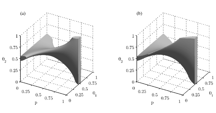
Figure 1. Let $f_{\theta}(x)=e^{-2(x-\theta)^{2}}$, $f^{\star}=f_{0.5}$, $\mathcal{M}_{2}=\{pf_{\theta_{1}}+(1-p)f_{\theta_{2}}:p,\theta_{1},\theta_{2}\in[0,1]\}$. The plots illustrate (a) the set of parameters $(p,\theta_{1},\theta_{2})$ corresponding to the Hellinger ball $\{f\in\mathcal{M}_{2}:h(f,f^{\star})\leq 0.05\}$; and (b) the parameter set $\{(p,\theta_{1},\theta_{2}):N(p,\theta_{1},\theta_{2})\leq 0.05\}$ with $N(p,\theta_{1},\theta_{2})=|p(\theta_{1}-0.5)+(1-p)(\theta_{2}-0.5)|+\tfrac{1}{2}p(\theta_{1}-0.5)^{2}+\tfrac{1}{2}(1-p)(\theta_{2}-0.5)^{2}$. The two plots are related by the local geometry Theorem 3.10, which yields $c^{\star}N(p,\theta_{1},\theta_{2})\leq h(pf_{\theta_{1}}+(1-p)f_{\theta_{2}},f^{\star})\leq C^{\star}N(p,\theta_{1},\theta_{2})$.

The phenomenon illustrated in this example can be stated more generally. For $f^{\star}\in\mathcal{M}_{q^{\star}}$ such that $q^{\star}<q$ (note that $f^{\star}\in\mathcal{M}_{q}$ as $\mathcal{M}_{q}\subset\mathcal{M}_{q+1}$ for all $q$), the subset of parameters $\Xi_{q}(\delta)\subset\Xi_{q}$ corresponding to the ball $\mathcal{M}_{q}(\delta)=\{f\in\mathcal{M}_{q}:d(f,f^{\star})\leq\delta\}$ behaves nothing at all like a ball in a finite-dimensional Banach space (see Figure 1(a)): indeed, the diameter of $\Xi_{q}(\delta)$ is even bounded away from zero as $\delta\downarrow 0$. There is therefore no hope to deduce a local entropy bound of the form (1.2) for $N(\mathcal{M}_{q}(\delta),\varepsilon)$ directly from the corresponding bound in $\mathbb{R}^{qd+q-1}\supset\Xi_{q}$. This provides a vivid illustration of the difficulty of establishing local entropy bounds in geometrically irregular settings. Nevertheless, we will be able to obtain local entropy bounds for the mixture classes $\mathcal{M}_{q}$ in section 3 below.

For concreteness, we endow $\mathcal{M}_{q}$ with the Hellinger metric $h(f,g)=\|\sqrt{f}-\sqrt{g}\|_{L^{2}}$, which is the relevant metric for statistical applications [19, ch. 7], [17] (however, our results are easily adapted to other commonly used probability metrics—the total variation metric $d_{\rm TV}(f,g)=\|f-g\|_{L^{1}}$, for example—using almost identical proofs). The main result, Theorem 3.3, provides an explicit bound of the form (1.2) for $\mathcal{M}_{q}$ under suitable smoothness assumptions on $f_{0}$.

The fundamental challenge that we face in the proof is to develop a sharp quantitative understanding of the local geometry of mixtures (illustrated in Figure 1). The key result that we prove in this direction is Theorem 3.10, which forms the central contribution of this paper. As this result is rather technical, we postpone its description to section 3.2 below. However, an important consequence of this result is as follows: given a mixture $f^{\star}=\sum_{i=1}^{q^{\star}}\pi_{i}^{\star}f_{\theta_{i}^{\star}}$, one can choose sufficiently small neighborhoods $A_{1},\ldots,A_{q^{\star}}$ of $\theta_{1},\ldots,\theta_{q^{\star}}$, respectively, such that for any $q\geq 1$ and mixture $f=\sum_{i=1}^{q}\pi_{i}f_{\theta_{i}}$, the Hellinger metric $h(f,f^{\star})$ is of the same order as

$$\sum_{\theta_{j}\in A_{0}}\pi_{j}+\sum_{i=1}^{q^{\star}}\Bigg{\{}\Bigg{|}\sum_{\theta_{j}\in A_{i}}\pi_{j}-\pi_{i}^{\star}\Bigg{|}\\ \mbox{}+\Bigg{\|}\sum_{\theta_{j}\in A_{i}}\pi_{j}(\theta_{j}-\theta_{i}^{\star})\Bigg{\|}+\frac{1}{2}\sum_{\theta_{j}\in A_{i}}\pi_{j}\|\theta_{j}-\theta_{i}^{\star}\|^{2}\Bigg{\}}$$

(here $A_{0}=\mathbb{R}^{d}\backslash(A_{1}\cup\cdots\cup A_{q^{\star}})$). This pseudodistance controls precisely the set of parameters in $\Xi_{q}$ with density close to $f^{\star}$, see Figure 1 for an example.

Let us emphasize that while the local geometry theorem relates the Hellinger metric on $\mathcal{M}_{q}$ to a pseudodistance on $\Xi_{q}$, the latter is not a norm or even a metric. It is therefore still not possible to control the local entropy of $\mathcal{M}_{q}$ as in the case where the metric is comparable to a norm on $\Xi_{q}$. Instead, we deduce the local entropy bound in two steps. First, we observe that the local geometry theorem allows us to obtain a global entropy bound of the form (1.1) for the class of weighted densities

$$\mathcal{D}_{q}=\bigg{\{}\frac{\sqrt{f/f^{\star}}-1}{h(f,f^{\star})}:f\in\mathcal{M}_{q},~{}f\neq f^{\star}\bigg{\}},$$

as the above pseudodistance controls the coefficients in the Taylor expansion of $f$. This is accomplished in Theorem 3.1. The global entropy bound for $\mathcal{D}_{q}$ now yields a local entropy bound for $\mathcal{M}_{q}$ using a slicing procedure. The latter is not specific to mixtures, and will be developed first in a general setting in section 2.

Beside their intrinsic interest, the results in this paper are of direct relevance to statistical applications. Many problems in statistics and probability make use of estimates on the metric entropy of classes of densities: metric entropy controls the rate of convergence of uniform limit theorems in probability, and is therefore of central importance in the design and analysis of statistical estimators [20, 19, 17]. Such applications frequently require a slightly stronger notion of metric entropy known as bracketing entropy, which we will consider throughout this paper; see section 2. In infinite-dimensional situations, the global entropy is chiefly of interest: global entropy estimates for various classes of probability densities can be found in [20, 19, 17, 3, 9]. However, in finite-dimensional settings, global entropy bounds are known to yield sub-optimal results, and here local entropy bounds are essential to obtain optimal convergence rates of estimators [19, §7.5]. In the case of mixtures, the difficulty of obtaining local entropy bounds was noted, e.g., in [12, 18]. Applications of the results in this paper are given in [11, 10].

2. From global entropy to local entropy

The classical notion of covering numbers $N(T,\varepsilon)$ was defined in the introduction. We will consider throughout this paper a somewhat finer notion of covering by brackets (order intervals) rather than by balls. In this section, we will work in the general setting of normed vector lattices (normed Riesz spaces, see [1]).

Definition 2.1.

Let $(X,\|\cdot\|)$ be a normed vector lattice. For any subset $T\subseteq X$ and $\varepsilon>0$, the bracketing number $N_{[]}(T,\varepsilon)$ is defined as

$$N_{[]}(T,\varepsilon)=\inf\bigg{\{}n:\exists~{}l_{i},u_{i}\in X,~{}\|u_{i}-l_{i}\|\leq\varepsilon,~{}i=1,\ldots,n\mbox{ s.t.\ }T\subseteq\bigcup_{i=1}^{n}[l_{i},u_{i}]\bigg{\}},$$

where $[l,u]=\{x\in X:l\leq x\leq u\}$.

Note that as $[l,u]\subset B(l,\|u-l\|)$, it is evident that $N(T,\varepsilon)\leq N_{[]}(T,\varepsilon)$ for any $T\subseteq X$ and $\varepsilon>0$. Bounds on the bracketing number therefore imply bounds on the covering number, but not conversely. The finer covering by brackets is essential in many probabilistic and statistical applications [20, 19, 17].

Let $(X,\|\cdot\|)$ be a normed vector lattice, and let us fix a subset $T\subseteq X$ and a distinguished point $t_{0}\in T$. Our general aim is to obtain an estimate on the local covering (or bracketing) number $N(T\cap B(t_{0},\delta),\varepsilon)$ that is polynomial in $\delta/\varepsilon$. As is explained in the introduction, such estimates can be much more difficult to obtain than the corresponding estimates on the global covering number $N(T,\varepsilon)$ that are polynomial in $1/\varepsilon$. Unfortunately, the latter is strictly weaker than the former.

Nonetheless, global covering estimates can be useful. For any $t\neq t_{0}$, define

$$d_{t}=\frac{t-t_{0}}{\|t-t_{0}\|},\qquad\quad D_{0}=\{d_{t}:t\in T,~{}t\neq t_{0}\}.$$

The main message of this section is that a local covering estimate for $T$ can be obtained from a global covering estimate for the weighted class $D_{0}\subseteq X$. As global entropy estimates can be much easier to obtain than local entropy estimates, this provides a useful approach to obtaining local entropy bounds for geometrically complex classes. We state a precise result for bracketing numbers as will be needed in the sequel; a trivial modification of the proof yields a version for covering numbers. In the next section, this result will be applied in the context of mixtures.

Theorem 2.2.

Let $(X,\|\cdot\|)$ be a normed vector lattice. Fix $T\subseteq X$ and $t_{0}\in T$, and let $D_{0}$ be as above. Suppose that there exist $q,C_{0}\geq 1$ and $\varepsilon_{0}>0$ such that

$$N_{[]}(D_{0},\varepsilon)\leq\bigg{(}\frac{C_{0}}{\varepsilon}\bigg{)}^{q}\quad\mbox{for every }\varepsilon\leq\varepsilon_{0}.$$

Choose any $d\in X$ such that $|d_{t}|\leq d$ for all $t\in T$, $t\neq t_{0}$. Then

$$N_{[]}(T\cap B(t_{0},\delta),\rho)\leq\bigg{(}\frac{8C\delta}{\rho}\bigg{)}^{q+1}$$

for all $\delta,\rho>0$ such that $\rho/\delta<4\wedge 2\|d\|$, where $C=C_{0}(1\vee\|d\|/4\varepsilon_{0})$.

Remark 2.3.

Theorem 2.2 requires an upper bound $d\in X$ on $|D_{0}|$, that is, $D_{0}$ must be order-bounded. But the assumptions of the Theorem already require that $N_{[]}(D_{0},\varepsilon_{0})<\infty$, which is easily seen to imply order-boundedness of $D_{0}$. The latter therefore does not need to be added as a separate assumption.

Remark 2.4.

In Theorem 2.2, a global covering bound for $D_{0}$ of order $(1/\varepsilon)^{q}$ gives a local covering bound for $T$ of order $(\delta/\varepsilon)^{q+1}$. It is instructive to note that this polynomial scaling cannot be improved. Indeed, let $T$ be the unit (Euclidean) ball in $\mathbb{R}^{q+1}$, and let $t_{0}=0$. Then $D_{0}$ is the unit sphere in $\mathbb{R}^{q+1}$ and therefore has Kolmogorov dimension $q$, but the covering number of $B(0,\delta)$ is of order $(\delta/\varepsilon)^{q+1}$. The same conclusion holds also for bracketing (rather than covering) numbers.

Remark 2.5.

A natural question is whether a converse to the above results can be obtained. In general, however, this is not possible: the class $D_{0}$ can be much richer than the original class $T$, as the following simple example illustrates. Let $(X,\|\cdot\|)$ be an infinite-dimensional Hilbert lattice and let $(e_{k})_{k\geq 1}$ be an orthonormal basis. Let $T=\{2^{-k}e_{k}:k\geq 1\}\cup\{0\}$ and $t_{0}=0$. Then $N_{[]}(T\cap B(t_{0},2^{-r}),2^{-k})\leq k-r+1$ for $k\geq r$, so $N_{[]}(T\cap B(t_{0},\delta),\varepsilon)\leq\log_{2}(8\delta/\varepsilon)\leq(8\delta/\varepsilon)^{3/2}$ for all $\varepsilon/\delta\leq 1$. But here we have $D_{0}=\{e_{k}:k\geq 1\}$, so $N_{[]}(D_{0},\varepsilon)\geq N(D_{0},\varepsilon)=\infty$ for $\varepsilon>0$ small enough.

We now proceed to the proof of Theorem 2.2. The main idea of the proof is to partition the set $T\cap B(t_{0},\delta)$ into shells $\{t\in T:r^{-n}\delta\leq\|t-t_{0}\|\leq r^{-n+1}\delta\}$ for a suitable choice of $r>0$. The bracketing number of each shell is then controlled by that of the normalized class $D_{0}$ at scale $\sim r^{n}\rho/\delta$. Such a slicing procedure is commonly used in the reverse direction in the theory of weighted empirical processes (see, e.g., [19, sec. 5.3]). Here we apply this idea directly to the bracketing numbers.

Proof of Theorem 2.2.

The assumption implies that

$$N_{[]}(D_{0},\varepsilon)\leq\bigg{(}\frac{C_{0}}{\varepsilon\wedge\varepsilon_{0}}\bigg{)}^{q}\quad\mbox{for every }\varepsilon>0.$$

If $\varepsilon<\|d\|/4$, then

$$\frac{\varepsilon}{\varepsilon\wedge\varepsilon_{0}}\leq 1\vee\frac{\|d\|}{4\varepsilon_{0}}.$$

We therefore have

$$N_{[]}(D_{0},\varepsilon)\leq\bigg{(}\frac{C}{\varepsilon}\bigg{)}^{q}\quad\mbox{for every }\varepsilon<\|d\|/4,$$

where $C$ is as defined in the Theorem. This estimate will be used below.

Fix $\varepsilon,\delta>0$ and let $N=N_{[]}(D_{0},\varepsilon)$. Then there exist $l_{1},u_{1},\ldots,l_{N},u_{N}\in X$ such that $\|u_{i}-l_{i}\|\leq\varepsilon$ for all $i=1,\ldots,N$, and for every $t\in T$, $t\neq t_{0}$ there is an $1\leq i\leq N$ such that $l_{i}\leq d_{t}\leq u_{i}$. Choose $t\in T$ such that $r^{-n}\delta\leq\|t-t_{0}\|\leq r^{-n+1}\delta$ (with $r>1$ to be chosen later). Then there exists $1\leq i\leq N$ so that

$$(r^{-n}l_{i}\wedge r^{-n+1}l_{i})\,\delta+t_{0}\leq t\leq(r^{-n}u_{i}\vee r^{-n+1}u_{i})\,\delta+t_{0}.$$

Note that

$$\|u_{i}\,r^{-n}\delta-l_{i}\,r^{-n}\delta\| \leq r^{-n}\delta\varepsilon,$$

$$\|u_{i}\,r^{-n+1}\delta-l_{i}\,r^{-n+1}\delta\| \leq r^{-n+1}\delta\varepsilon,$$

$$\|u_{i}\,r^{-n+1}\delta-l_{i}\,r^{-n}\delta\| \leq(r-1)r^{-n}\delta+r^{-n+1}\delta\varepsilon,$$

$$\|u_{i}\,r^{-n}\delta-l_{i}\,r^{-n+1}\delta\| \leq(r-1)r^{-n}\delta+r^{-n+1}\delta\varepsilon,$$

where the latter two estimates follow from $l_{i}\leq d_{t}\leq u_{i}$, $\|d_{t}\|=1$, and

$$(u_{i}-l_{i})\,r^{-n}\delta \leq u_{i}\,r^{-n+1}\delta-l_{i}\,r^{-n}\delta-d_{t}\,(r-1)r^{-n}\delta\leq(u_{i}-l_{i})\,r^{-n+1}\delta,$$

$$(u_{i}-l_{i})\,r^{-n}\delta \leq u_{i}\,r^{-n}\delta-l_{i}\,r^{-n+1}\delta+d_{t}\,(r-1)r^{-n}\delta\leq(u_{i}-l_{i})\,r^{-n+1}\delta.$$

As $|a\vee b-c\wedge d|\leq|a-c|+|a-d|+|b-c|+|b-d|$, we can estimate

$$\|(r^{-n}u_{i}\vee r^{-n+1}u_{i})\,\delta-(r^{-n}l_{i}\wedge r^{-n+1}l_{i})\,\delta\|\leq 2(r-1)r^{-n}\delta+4r^{-n+1}\delta\varepsilon.$$

Therefore, we have shown that

$$N_{[]}(\{t\in T:r^{-n}\delta\leq\|t-t_{0}\|\leq r^{-n+1}\delta\},2(r-1)r^{-n}\delta+4r^{-n+1}\delta\varepsilon)\leq N_{[]}(D_{0},\varepsilon)$$

for arbitrary $\varepsilon,\delta>0$, $r>1$, $n\in\mathbb{N}$. In particular,

$$N_{[]}(\{t\in T:r^{-n}\delta\leq\|t-t_{0}\|\leq r^{-n+1}\delta\},\rho)\leq N_{[]}(D_{0},\tfrac{1}{4}r^{n-1}\rho/\delta-\tfrac{1}{2}(1-1/r))$$

for every $\delta>0$, $r>1$, $n\in\mathbb{N}$, $\rho>2(r-1)r^{-n}\delta$.

Choose an envelope $d\in X$ such that $|d_{t}|\leq d$ for all $t\in T$, $t\neq t_{0}$. Evidently

$$t_{0}-r^{-n}\delta\,d\leq t\leq t_{0}+r^{-n}\delta\,d$$

for all $t\in T$ such that $\|t-t_{0}\|\leq r^{-n}\delta$. Therefore

$$N_{[]}(\{t\in T:\|t-t_{0}\|\leq r^{-\lceil H\rceil}\delta\},2r^{-H}\delta\|d\|)=1$$

for all $\delta>0$, $r>1$, $H>0$. Thus we can estimate

$$N_{[]}(T\cap B(t_{0},\delta),2r^{-H}\delta\|d\|)$$

$$\quad\leq 1+\sum_{n=1}^{\lceil H\rceil}N_{[]}(\{t\in T:r^{-n}\delta\leq\|t-t_{0}\|\leq r^{-n+1}\delta\},2r^{-H}\delta\|d\|)$$

$$\quad\leq 1+\sum_{n=1}^{\lceil H\rceil}N_{[]}(D_{0},\{r^{n-H-1}\|d\|-(1-1/r)\}/2)$$

whenever $\delta>0$, $r>1$, $H>0$ such that $\|d\|>(1-1/r)r^{H}$. In particular,

$$N_{[]}(T\cap B(t_{0},\delta),2r^{-H}\delta\|d\|)\leq 1+\sum_{n=1}^{\lceil H\rceil}N_{[]}(D_{0},r^{n-H-1}\|d\|/4)$$

whenever $\delta>0$, $r>1$, $H>0$ such that $\|d\|\geq 2(1-1/r)r^{H}$, where we have used that the bracketing number is a nonincreasing function of the bracket size.

Now recall that

$$N_{[]}(D_{0},\varepsilon)\leq\bigg{(}\frac{C}{\varepsilon}\bigg{)}^{q}\quad\mbox{for every }0<\varepsilon<\|d\|/4,$$

where $q,C\geq 1$. Thus

$$N_{[]}(T\cap B(t_{0},\delta),2r^{-H}\delta\|d\|)\leq 1+\sum_{n=1}^{\lceil H\rceil}r^{-(n-1)q}\bigg{(}\frac{8C}{2r^{-H}\|d\|}\bigg{)}^{q}$$

whenever $\delta>0$, $r>1$, $H>0$ such that $\|d\|\geq 2(1-1/r)r^{H}$. But

$$\sum_{n=1}^{\lceil H\rceil}r^{-(n-1)q}\leq\frac{1}{1-1/r^{q}}\leq\frac{1}{1-1/r}\leq\frac{\|d\|}{2(1-1/r)r^{H}}\frac{4C}{2r^{-H}\|d\|}$$

as $r>1$ and $q,C\geq 1$. We can therefore estimate

$$N_{[]}(T\cap B(t_{0},\delta),2r^{-H}\delta\|d\|)\leq\frac{\|d\|}{2(1-1/r)r^{H}}\bigg{(}\frac{8C}{2r^{-H}\|d\|}\bigg{)}^{q+1}$$

whenever $\delta>0$, $r>1$, $H>0$ such that $\|d\|\geq 2(1-1/r)r^{H}$.

We now fix $\delta,\rho>0$ such that $\rho/\delta<4\wedge 2\|d\|$, and choose

$$r=\frac{4}{4-\rho/\delta},\qquad H=\frac{\log(2\|d\|\delta/\rho)}{\log r}.$$

Clearly $r>1$ and $H>0$. Moreover, note that our choice of $r$ and $H$ implies that $\|d\|=2(1-1/r)r^{H}$ and $\rho=2r^{-H}\delta\|d\|$. We have therefore shown that

$$N_{[]}(T\cap B(t_{0},\delta),\rho)\leq\bigg{(}\frac{8C\delta}{\rho}\bigg{)}^{q+1}$$

for all $\delta,\rho>0$ such that $\rho/\delta<4\wedge 2\|d\|$. ∎

3. The local entropy of mixtures

3.1. Definitions and main results

Let $\mu$ be the Lebesgue measure on $\mathbb{R}^{d}$. We fix a positive probability density $f_{0}$ with respect to $\mu$ ($f_{0}>0$ and $\int f_{0}d\mu=1$), and consider mixtures (finite convex combinations) of densities in the class

$$\{f_{\theta}:\theta\in\mathbb{R}^{d}\},\qquad f_{\theta}(x)=f_{0}(x-\theta)\quad\forall\,x\in\mathbb{R}^{d}.$$

In everything that follows we fix a nondegenerate mixture $f^{\star}$ of the form

$$f^{\star}=\sum_{i=1}^{q^{\star}}\pi_{i}^{\star}f_{\theta_{i}^{\star}}.$$

Nondegenerate means that $\pi_{i}^{\star}>0$ for all $i$, and $\theta_{i}^{\star}\neq\theta_{j}^{\star}$ for all $i\neq j$.

Let $\Theta\subset\mathbb{R}^{d}$ be a bounded parameter set such that $\{\theta^{\star}_{i}:i=1,\ldots,q^{\star}\}\subseteq\Theta$, and denote its diameter by $2T$ (that is, $\Theta$ is included in some closed Euclidean ball of radius $T$). We consider for $q\geq 1$ the family of $q$-mixtures

$$\mathcal{M}_{q}=\bigg{\{}\sum_{i=1}^{q}\pi_{i}f_{\theta_{i}}:\pi_{i}\geq 0,~{}\sum_{i=1}^{q}\pi_{i}=1,~{}\theta_{i}\in\Theta\bigg{\}}.$$

The goal of this section is to obtain a local entropy bound for $\mathcal{M}_{q}$ at the point $f^{\star}$, where $\mathcal{M}_{q}$ is endowed with the Hellinger metric

$$h(f,g)=\bigg{[}\int\big{(}\textstyle{\sqrt{f}-\sqrt{g}}\big{)}^{2}d\mu\bigg{]}^{1/2},\qquad f,g\in\mathcal{M}_{q}.$$

That is, we seek bounds on quantities such as $N_{h}(\{f\in\mathcal{M}_{q}:h(f,f^{\star})\leq\varepsilon\},\delta)$, where $N_{h}$ denotes the covering number in the metric space $(\mathcal{M}_{q},h)$ (i.e., covering by Hellinger balls). In fact, we prove a stronger bound of bracketing type. Our choice of the Hellinger metric and the particular form of the bracketing number to be considered is directly motivated by statistical applications [19, ch. 7], [17, §7.4]; see [11, 10] for statistical applications of the results below. We will adhere to this setting for concreteness, though other metrics may similarly be considered.

In the sequel, we denote by $\|\cdot\|_{p}$ the $L^{p}(f^{\star}d\mu)$-norm, that is, $\|g\|_{p}^{p}=\int|g|^{p}f^{\star}d\mu$. Note that the Hellinger metric can be written as $h(f,g)=\|\sqrt{f/f^{\star}}-\sqrt{g/f^{\star}}\|_{2}$. To obtain covering bounds for $\mathcal{M}_{q}$ in the Hellinger metric, we can therefore apply the results of section 2 for the case where $(X,\|\cdot\|)$ is the Banach lattice $(L^{2}(f^{\star}d\mu),\|\cdot\|_{2})$, $T=\{\sqrt{f/f^{\star}}:f\in\mathcal{M}_{q}\}$, and $t_{0}=1$. Indeed, it is easily seen that

$$N_{h}(\{f\in\mathcal{M}_{q}:h(f,f^{\star})\leq\varepsilon\},2\delta)\leq N(\mathcal{H}_{q}(\varepsilon),\delta)\leq N_{[]}(\mathcal{H}_{q}(\varepsilon),\delta),$$

where we have defined

$$\mathcal{H}_{q}(\varepsilon)=\{\sqrt{f/f^{\star}}:f\in\mathcal{M}_{q},~{}\|\sqrt{f/f^{\star}}-1\|_{2}\leq\varepsilon\}\subset L^{2}(f^{\star}d\mu).$$

Our aim is to obtain a polynomial bound for the bracketing number $N_{[]}(\mathcal{H}_{q}(\varepsilon),\delta)$. To this end, we will apply Theorem 2.2 to the weighted class $\mathcal{D}_{q}$ defined by

$$\mathcal{D}_{q}=\{d_{f}:f\in\mathcal{M}_{q},~{}f\neq f^{\star}\},\qquad\quad d_{f}=\frac{\sqrt{f/f^{\star}}-1}{\|\sqrt{f/f^{\star}}-1\|_{2}}.$$

The essential difficulty is now to control the global entropy of $\mathcal{D}_{q}$.

The following notation will be used throughout:

$$H_{0}(x) =\sup_{\theta\in\Theta}f_{\theta}(x)/f^{\star}(x),$$

$$H_{1}(x) =\sup_{\theta\in\Theta}\max_{i=1,\ldots,d}|\partial f_{\theta}(x)/\partial\theta^{i}|/f^{\star}(x),$$

$$H_{2}(x) =\sup_{\theta\in\Theta}\max_{i,j=1,\ldots,d}|\partial^{2}f_{\theta}(x)/\partial\theta^{i}\partial\theta^{j}|/f^{\star}(x),$$

$$H_{3}(x) =\sup_{\theta\in\Theta}\max_{i,j,k=1,\ldots,d}|\partial^{3}f_{\theta}(x)/\partial\theta^{i}\partial\theta^{j}\partial\theta^{k}|/f^{\star}(x)$$

when $f_{0}$ is sufficiently differentiable, $\mathcal{M}=\bigcup_{q\geq 1}\mathcal{M}_{q}$, and $\mathcal{D}=\bigcup_{q\geq 1}\mathcal{D}_{q}$.

Assumption A.

The following hold:

1. $f_{0}\in C^{3}$ and $f_{0}(x)$, $(\partial f_{0}/\partial\theta^{i})(x)$ vanish as $\|x\|\to\infty$.

2. $H_{k}\in L^{4}(f^{\star}d\mu)$ for $k=0,1,2$ and $H_{3}\in L^{2}(f^{\star}d\mu)$.

We can now state our main result, whose proof is given in section 3.3.

Theorem 3.1.

Suppose that Assumption A holds. Then there exist constants $C^{\star}$ and $\delta^{\star}$, which depend on $d$, $q^{\star}$ and $f^{\star}$ but not on $\Theta$, $q$ or $\delta$, such that

$$N_{[]}(\mathcal{D}_{q},\delta)\leq\bigg{(}\frac{C^{\star}(T\vee 1)^{1/3}(\|H_{0}\|_{4}^{4}\vee\|H_{1}\|_{4}^{4}\vee\|H_{2}\|_{4}^{4}\vee\|H_{3}\|_{2}^{2})}{\delta}\bigg{)}^{10(d+1)q}$$

for all $q\geq q^{\star}$, $\delta\leq\delta^{\star}$. Moreover, there is a function $D\in L^{4}(f^{\star}d\mu)$ with

$$\|D\|_{4}\leq K^{\star}(\|H_{0}\|_{4}\vee\|H_{1}\|_{4}\vee\|H_{2}\|_{4}),$$

where $K^{\star}$ depends only on $d$ and $f^{\star}$, such that $|d|\leq D$ for all $d\in\mathcal{D}$.

Remark 3.2.

Assumption A is essentially a smoothness assumption on $f_{0}$. Some sort of smoothness is certainly needed for a result such as Theorem 3.1 to hold: see [5, §3] for a counterexample in the non-smooth case.

Combining Theorems 2.2 and 3.1, we immediately obtain a local entropy bound.

Theorem 3.3.

Suppose that Assumption A holds. Then

$$N_{[]}(\mathcal{H}_{q}(\varepsilon),\delta)\leq\bigg{(}\frac{C_{\Theta}\,\varepsilon}{\delta}\bigg{)}^{10(d+1)q+1}$$

for all $q\geq q^{\star}$ and $\delta/\varepsilon\leq 1$, where

$$C_{\Theta}=L^{\star}\,(T\vee 1)^{1/3}\,(\|H_{0}\|_{4}^{4}\vee\|H_{1}\|_{4}^{4}\vee\|H_{2}\|_{4}^{4}\vee\|H_{3}\|_{2}^{2})^{5/4}$$

and $L^{\star}$ is a constant that depends only on $d$, $q^{\star}$ and $f^{\star}$.

To illustrate these results, let us consider the important case of Gaussian location mixtures, which are widely used in applications (see, e.g., [12, 13, 18]).

Example 3.4 (Gaussian mixtures).

Consider mixtures of standard Gaussian densities $f_{0}(x)=(2\pi)^{-d/2}e^{-\|x\|^{2}/2}$, and let $\Theta(T)=\{\theta\in\mathbb{R}^{d}:\|\theta\|\leq T\}$. Fix a nondegenerate mixture $f^{\star}$, and define $T^{\star}=\max_{i=1,\ldots,q^{\star}}\|\theta_{i}^{\star}\|$. Denote by $\mathcal{H}_{q}(\varepsilon,T)$ the Hellinger ball associated to the parameter set $\Theta(T)$. Then

$$N_{[]}(\mathcal{H}_{q}(\varepsilon,T),\delta)\leq\bigg{(}\frac{C_{1}^{\star}e^{C_{2}^{\star}T^{2}}\varepsilon}{\delta}\bigg{)}^{10(d+1)q+1}$$

for all $q\geq q^{\star}$, $T\geq T^{\star}$, and $\delta/\varepsilon\leq 1$, where $C_{1}^{\star},C_{2}^{\star}$ are constants that depend on $d$, $q^{\star}$ and $f^{\star}$ only. To prove this, it evidently suffices to show that Assumption A holds and that $\|H_{k}\|_{4}$ for $k=0,1,2$ and $\|H_{3}\|_{2}$ are of order $e^{CT^{2}}$. These facts are readily verified by a straightforward computation.

Let us emphasize a key feature of Theorems 3.1 and 3.3: the dependence of the entropy bounds on the order $q$ and on the parameter set $\Theta$ is explicit (see, e.g., Example 3.4). In particular, we find that for every $f^{\star}$, the local doubling dimension of $\mathcal{M}_{q}$ at $f^{\star}$ is of the same order as the dimension of the natural parameter set for mixtures $\Delta_{q-1}\times\Theta^{q}$, which answers the basic question posed in the introduction. Obtaining this explicit dependence, which is important in applications [11], is one of the main technical challenges of the proof. In order to show only that $N_{[]}(\mathcal{H}_{q}(\varepsilon),\delta)$ is polynomial in $\varepsilon/\delta$ without explicit control of the order, the proof could be simplified and substantially generalized—see Remark 3.6 below for some discussion. In contrast to the dependence on $q$ and $\Theta$, however, the proofs of Theorems 3.1 and 3.3 do not provide any control of the dependence of the constants on $f^{\star}$. In particular, while we can control the local doubling dimension of $\mathcal{M}_{q}$ at $f^{\star}$ in terms of $q$, we do not know whether the dependence on $f^{\star}$ can be eliminated.

Remark 3.5.

We have not optimized the constants in Theorem 3.1 and Theorem 3.3. In particular, the constant $10$ in the exponent can likely be improved. On the other hand, it is unclear whether the dependence on the diameter of $\Theta$ is optimal. Indeed, if one is only interested in global entropy $N_{[]}(\mathcal{H}_{q},\delta)$ where $\mathcal{H}_{q}=\{\sqrt{f/f^{\star}}:f\in\mathcal{M}_{q}\}$, then it can be read off from the proof of Theorem 3.1 that the constants in the entropy bound depend on $\|H_{0}\|_{1}$ and $\|H_{1}\|_{1}$ only, which are easily seen to scale polynomially in $T$ due to the translation invariance of the Lebesgue measure. Therefore, for example in the case of Gaussian mixtures, one can obtain a global entropy bound which scales only polynomially as a function of $T$, whereas the above local entropy bound scales as $e^{CT^{2}}$. The behavior of local entropies is much more delicate than that of global entropies, however, and we do not know whether it is possible to obtain a local entropy bound that scales polynomially in $T$ for the Hellinger metric. On the other hand, if $\mathcal{M}_{q}$ is endowed with the total variation metric $d_{\rm TV}(f,g)=\int|f-g|d\mu$ rather than the Hellinger metric, then an easy modification of our proof yields a local entropy bound that depends only on $\|H_{i}\|_{1}$ ($i=0,\ldots,3$), and therefore scales polynomially in $T$. In this case the scaling matches that of the global entropy, and is therefore optimal.

Remark 3.6.

The problems that we address in this section could be investigated in a more general setting. Let $\mathcal{F}=\{f_{\theta}:\theta\in\Theta\}$ be a given family of probability densities (where $\Theta$ is a bounded subset of $\mathbb{R}^{d}$), and define

$$\mathcal{M}_{q}=\bigg{\{}\sum_{i=1}^{q}\pi_{i}f_{\theta_{i}}:\pi_{i}\geq 0,~{}\sum_{i=1}^{q}\pi_{i}=1,~{}\theta_{i}\in\Theta\bigg{\}}.$$

The case that we have considered corresponds to the choice $\mathcal{F}=\{f_{0}(\,\cdot\,-\theta):\theta\in\Theta\}$, but in principle any parametrized family $\mathcal{F}$ may be considered.

Remarkably, most of the proof of Theorem 3.1 does not rely at all on the specific choice of $\mathcal{F}$, so that very similar techniques may be used to study more general mixtures. The only point where the structure of $\mathcal{F}$ has been used is in the local geometry Theorem 3.10 below, whose proof (using Fourier methods) relies on the specific form of location mixtures. We believe that essentially the same result holds more generally, but a different method of proof would likely be needed.

The proof of Theorem 3.10 below is rather technical: the difficulty lies in the fact that the result holds uniformly in the order $q$. This is necessary in order to obtain bounds in Theorems 3.1 and 3.3 that depend explicitly on $q$. If the explicit dependence on $q$ is not needed, then our proof of Theorem 3.10 can be simplified and adapted to hold for much more general classes $\mathcal{F}$, see [10].

Finally, we note that $\mathcal{M}=\bigcup_{q}\mathcal{M}_{q}$ is simply the convex hull of $\mathcal{F}$. The problem of estimating the metric entropy of convex hulls has been widely studied [4, 7, 8, 12, 13]. In general, however, the convex hull is infinite-dimensional, so that this problem is quite distinct from the problems we have considered.

Remark 3.7.

Weighted entropy bounds as in Theorem 3.1 are of independent interest. A qualitative version of this bound (without uniform control in $q$ and $T$) was assumed in [6], which provided inspiration for the present effort. However, in [6, Prop. 3.1], it is assumed without justification that one can choose a multiplicative rather than additive remainder term in a Taylor expansion. The requisite justification is provided (in a much more precise form) by the local geometry theorem to be described presently. Developing a precise understanding of the local geometry of mixtures is the fundamental challenge to be surmounted in our setting, and our local geometry result therefore constitutes the central contribution of this paper.

3.2. The local geometry of mixtures

At the heart of the proof of Theorem 3.1 lies a result on the local geometry of location mixtures, Theorem 3.10 below. Before we can develop this result, we must introduce some notation.

Define the Euclidean balls $B(\theta,\varepsilon)=\{\theta^{\prime}\in\mathbb{R}^{d}:\|\theta-\theta^{\prime}\|<\varepsilon\}$, denote by $\langle u,v\rangle$ the inner product of two vectors $u,v\in\mathbb{R}^{d}$, and denote by $\langle A,u\rangle=\{\langle\theta,u\rangle:\theta\in A\}\subseteq\mathbb{R}$ the inner product of a set $A\subseteq\mathbb{R}^{d}$ with a vector $u\in\mathbb{R}^{d}$.

Lemma 3.8.

It is possible to choose a bounded convex neighborhood $A_{i}$ of $\theta_{i}^{\star}$ for every $i=1,\ldots,q^{\star}$ such that, for some linearly independent family $u_{1},\ldots,u_{d}\in\mathbb{R}^{d}$, the sets $\{\langle A_{i},u_{j}\rangle:i=1,\ldots,q^{\star}\}$ are disjoint for every $j=1,\ldots,d$.

Proof.

We first claim that one can choose linearly independent $u_{1},\ldots,u_{d}$ such that $|\{\langle\theta_{i}^{\star},u_{j}\rangle:i=1,\ldots,q^{\star}\}|=q^{\star}$ for every $j=1,\ldots,d$. Indeed, note that the set $\{u\in\mathbb{R}^{d}:|\{\langle\theta_{i}^{\star},u\rangle:i=1,\ldots,q^{\star}\}|<q^{\star}\}$ is a finite union of $(d-1)$-dimensional hyperplanes, which has Lebesgue measure zero. Therefore, if we draw a rotation matrix $T$ at random from the Haar measure on $\mathrm{SO}(d)$, and let $u_{i}=Te_{i}$ for all $i=1,\ldots,d$ where $\{e_{1},\ldots,e_{d}\}$ is the standard Euclidean basis in $\mathbb{R}^{d}$, then the desired property will hold with unit probability. To complete the proof, it suffices to choose $A_{i}=B(\theta_{i}^{\star},\varepsilon/4)$ with $\varepsilon=\min_{k}\min_{i\neq j}|\langle\theta_{i}^{\star}-\theta_{j}^{\star},u_{k}\rangle|$. ∎

We now fix once and for all a family of neighborhoods $A_{1},\ldots,A_{q^{\star}}$ as in Lemma 3.8. The precise choice of these sets only affects the constants in the proofs below and is therefore irrelevant to our final result; we only presume that $A_{1},\ldots,A_{q^{\star}}$ remain fixed throughout the proofs. Let us also define $A_{0}=\mathbb{R}^{d}\backslash(A_{1}\cup\cdots\cup A_{q^{\star}})$. Then $\{A_{0},\ldots,A_{q^{\star}}\}$ partitions the parameter set $\mathbb{R}^{d}$ in such a way that each bounded element $A_{i}$, $i=1,\ldots,q^{\star}$ contains precisely one component of the mixture $f^{\star}$, while the unbounded element $A_{0}$ contains no components of $f^{\star}$.

Let us define for each finite measure $\lambda$ on $\mathbb{R}^{d}$ the function

$$f_{\lambda}(x)=\int f_{\theta}(x)\,\lambda(d\theta).$$

We also define the derivatives $D_{1}f_{\theta}(x)\in\mathbb{R}^{d}$ and $D_{2}f_{\theta}(x)\in\mathbb{R}^{d\times d}$ as

$$[D_{1}f_{\theta}(x)]_{i}=\frac{\partial}{\partial\theta^{i}}f_{\theta}(x),\qquad[D_{2}f_{\theta}(x)]_{ij}=\frac{\partial^{2}}{\partial\theta^{i}\partial\theta^{j}}f_{\theta}(x).$$

Denote by $\mathfrak{P}(A)$ the space of probability measures supported on $A\subseteq\mathbb{R}^{d}$, and denote by $M_{+}^{d}$ the family of all $d\times d$ positive semidefinite (symmetric) matrices.

Definition 3.9.

Let us write

$$\mathfrak{D}=\{(\eta,\beta,\rho,\tau,\nu):\eta_{1},\ldots,\eta_{q^{\star}}\in\mathbb{R},~{}\beta_{1},\ldots,\beta_{q^{\star}}\in\mathbb{R}^{d},~{}\rho_{1},\ldots,\rho_{q^{\star}}\in M_{+}^{d},\\ \tau_{0},\ldots,\tau_{q^{\star}}\geq 0,~{}\nu_{0}\in\mathfrak{P}(A_{0}),\ldots,\nu_{q^{\star}}\in\mathfrak{P}(A_{q^{\star}})\}.$$

Then we define for each $(\eta,\beta,\rho,\tau,\nu)\in\mathfrak{D}$ the function

$$\ell(\eta,\beta,\rho,\tau,\nu)=\tau_{0}\frac{f_{\nu_{0}}}{f^{\star}}+\sum_{i=1}^{q^{\star}}\bigg{\{}\eta_{i}\frac{f_{\theta_{i}^{\star}}}{f^{\star}}+\beta_{i}^{*}\frac{D_{1}f_{\theta_{i}^{\star}}}{f^{\star}}+\mathrm{Tr}\bigg{[}\rho_{i}\frac{D_{2}f_{\theta_{i}^{\star}}}{f^{\star}}\bigg{]}+\tau_{i}\frac{f_{\nu_{i}}}{f^{\star}}\bigg{\}},$$

and the nonnegative quantity

$$N(\eta,\beta,\rho,\tau,\nu)=\tau_{0}+\sum_{i=1}^{q^{\star}}|\eta_{i}+\tau_{i}|+\sum_{i=1}^{q^{\star}}\bigg{\|}\beta_{i}+\tau_{i}\int(\theta-\theta_{i}^{\star})\,\nu_{i}(d\theta)\bigg{\|}+\mbox{}\\ \sum_{i=1}^{q^{\star}}\mathrm{Tr}[\rho_{i}]+\sum_{i=1}^{q^{\star}}\frac{\tau_{i}}{2}\int\|\theta-\theta_{i}^{\star}\|^{2}\nu_{i}(d\theta).$$

We now formulate the key result on the local geometry of the mixture class $\mathcal{M}$.

Theorem 3.10.

Suppose that

1. $f_{0}\in C^{2}$ and $f_{0}(x)$, $D_{1}f_{0}(x)$ vanish as $\|x\|\to\infty$.

2. $\|[D_{1}f_{0}]_{i}/f^{\star}\|_{1}<\infty$ and $\|[D_{2}f_{0}]_{ij}/f^{\star}\|_{1}<\infty$ for all $i,j=1,\ldots,d$.

Then there exists a constant $c^{\star}>0$ such that

$$\|\ell(\eta,\beta,\rho,\tau,\nu)\|_{1}\geq c^{\star}\,N(\eta,\beta,\rho,\tau,\nu)\quad\mbox{for all }(\eta,\beta,\rho,\tau,\nu)\in\mathfrak{D}.$$

[The constant $c^{\star}$ may depend on $f^{\star}$ and $A_{1},\ldots,A_{q^{\star}}$ but not on $\eta,\beta,\rho,\tau,\nu$.]

Before we turn to the proof, let us introduce a notion that is familiar in quantum mechanics. If $(\Omega,\Sigma)$ is a measurable space, call the map $\lambda:\Sigma\to\mathbb{R}^{d\times d}$ a state if

1. $A\mapsto[\lambda(A)]_{ij}$ is a signed measure for every $i,j=1,\ldots,d$;

2. $\lambda(A)$ is a nonnegative symmetric matrix for every $A\in\Sigma$;

3. $\mathrm{Tr}[\lambda(\Omega)]=1$.

It is easily seen that for any unit vector $\xi\in\mathbb{R}^{d}$, the map $A\mapsto\langle\xi,\lambda(A)\xi\rangle$ is a sub-probability measure. Moreover, if $\xi_{1},\ldots,\xi_{d}\in\mathbb{R}^{d}$ are linearly independent, there must be at least one $\xi_{i}$ such that $\langle\xi_{i},\lambda(\Omega)\xi_{i}\rangle>0$. Finally, let $B\subset\mathbb{R}^{d}$ be a compact set and let $(\lambda_{n})_{n\geq 0}$ be a sequence of states on $B$. Then there exists a subsequence along which $\lambda_{n}$ converges weakly to some state $\lambda$ on $B$ in the sense that $\int\mathrm{Tr}[M(\theta)\lambda_{n}(d\theta)]\to\int\mathrm{Tr}[M(\theta)\lambda(d\theta)]$ for every continuous function $M:B\to\mathbb{R}^{d\times d}$. To see this, it suffices to note that we may extract a subsequence such that all matrix elements $[\lambda_{n}]_{ij}$ converge weakly to a signed measure by the compactness of $B$, and it is evident that the limit must again define a state.

Proof of Theorem 3.10.

Suppose that the conclusion of the theorem does not hold. Then there must exist a sequence of coefficients $(\eta^{n},\beta^{n},\rho^{n},\tau^{n},\nu^{n})\in\mathfrak{D}$ with

$$\frac{\|\ell(\eta^{n},\beta^{n},\rho^{n},\tau^{n},\nu^{n})\|_{1}}{N(\eta^{n},\beta^{n},\rho^{n},\tau^{n},\nu^{n})}\xrightarrow{n\to\infty}0.$$

Let us fix such a sequence throughout the proof.

Applying Taylor’s theorem to $u\mapsto f_{\theta_{i}^{\star}+u(\theta-\theta_{i}^{\star})}$, we can write for $i=1,\ldots,q^{\star}$

$$\eta_{i}^{n}\frac{f_{\theta_{i}^{\star}}}{f^{\star}}+\beta_{i}^{n*}\frac{D_{1}f_{\theta_{i}^{\star}}}{f^{\star}}+\mathrm{Tr}\bigg{[}\rho_{i}^{n}\frac{D_{2}f_{\theta_{i}^{\star}}}{f^{\star}}\bigg{]}+\tau_{i}^{n}\frac{f_{\nu_{i}^{n}}}{f^{\star}}$$

$$\mbox{}=\left(\eta_{i}^{n}+\tau_{i}^{n}\right)\frac{f_{\theta_{i}^{\star}}}{f^{\star}}+\bigg{(}\beta_{i}^{n}+\tau_{i}^{n}\int(\theta-\theta_{i}^{\star})\,\nu_{i}^{n}(d\theta)\bigg{)}^{*}\frac{D_{1}f_{\theta_{i}^{\star}}}{f^{\star}}+\mathrm{Tr}\bigg{[}\rho_{i}^{n}\frac{D_{2}f_{\theta_{i}^{\star}}}{f^{\star}}\bigg{]}$$

$$\quad\mbox{}+\frac{\tau_{i}^{n}}{2}\int\|\theta-\theta_{i}^{\star}\|^{2}\,\nu_{i}^{n}(d\theta)\int\mathrm{Tr}\bigg{[}\bigg{\{}\int_{0}^{1}\frac{D_{2}f_{\theta_{i}^{\star}+u(\theta-\theta_{i}^{\star})}}{f^{\star}}\,2(1-u)\,du\bigg{\}}\,\lambda_{i}^{n}(d\theta)\bigg{]}$$

where $\lambda_{i}^{n}$ is the state on $A_{i}$ defined by

$$\int\mathrm{Tr}[M(\theta)\,\lambda_{i}^{n}(d\theta)]=\frac{\int\mathrm{Tr}[M(\theta)\,(\theta-\theta_{i}^{\star})(\theta-\theta_{i}^{\star})^{*}]\,\nu_{i}^{n}(d\theta)}{\int\|\theta-\theta_{i}^{\star}\|^{2}\,\nu_{i}^{n}(d\theta)}$$

(it is clearly no loss of generality to assume that $\nu_{i}^{n}$ has no mass at $\theta_{i}^{\star}$ for any $i,n$, so that everything is well defined). We now define the coefficients

$$\halign{\hbox to\displaywidth{$\hfil\displaystyle#\hfil$}\cr 0.0pt{\hfil$\displaystyle a_{i}^{n}=\frac{\eta_{i}^{n}+\tau_{i}^{n}}{N(\eta^{n},\beta^{n},\rho^{n},\tau^{n},\nu^{n})},\qquad b_{i}^{n}=\frac{\beta_{i}^{n}+\tau_{i}^{n}\int(\theta-\theta_{i}^{\star})\,\nu_{i}^{n}(d\theta)}{N(\eta^{n},\beta^{n},\rho^{n},\tau^{n},\nu^{n})},\cr 0.0pt{\hfil$\displaystyle c_{i}^{n}=\frac{\rho_{i}^{n}}{N(\eta^{n},\beta^{n},\rho^{n},\tau^{n},\nu^{n})},\qquad d_{i}^{n}=\frac{\frac{\tau_{i}^{n}}{2}\int\|\theta-\theta_{i}^{\star}\|^{2}\,\nu_{i}^{n}(d\theta)}{N(\eta^{n},\beta^{n},\rho^{n},\tau^{n},\nu^{n})}\crcr}}}$$

for $i=1,\ldots,q^{\star}$, and

$$a_{0}^{n}=\frac{\tau_{0}^{n}}{N(\eta^{n},\beta^{n},\rho^{n},\tau^{n},\nu^{n})}.$$

Note that

$$|a_{0}^{n}|+\sum_{i=1}^{q^{\star}}\left\{|a_{i}^{n}|+\|b_{i}^{n}\|+\mathrm{Tr}[c_{i}^{n}]+|d_{i}^{n}|\right\}=1$$

for all $n$. We may therefore extract a subsequence such that:

1. There exist $a_{i}\in\mathbb{R}$, $b_{i}\in\mathbb{R}^{d}$, $c_{i}\in M_{+}^{d}$, and $a_{0},d_{i}\geq 0$ (for $i=1,\ldots,q^{\star}$) with $|a_{0}|+\sum_{i=1}^{q^{\star}}\left\{|a_{i}|+\|b_{i}\|+\mathrm{Tr}[c_{i}]+|d_{i}|\right\}=1$, such that $a_{0}^{n}\to a_{0}$ and $a_{i}^{n}\to a_{i}$, $b_{i}^{n}\to b_{i}$, $c_{i}^{n}\to c_{i}$, $d_{i}^{n}\to d_{i}$ as $n\to\infty$ for all $i=1,\ldots,q^{\star}$.

2. There exists a sub-probability measure $\nu_{0}$ supported on $A_{0}$, such that $\nu_{0}^{n}$ converges vaguely to $\nu_{0}$ as $n\to\infty$.

3. There exist states $\lambda_{i}$ supported on $\mathop{\mathrm{cl}}A_{i}$ for $i=1,\ldots,q^{\star}$, such that $\lambda_{i}^{n}$ converges weakly to $\lambda_{i}$ as $n\to\infty$ for every $i=1,\ldots,q^{\star}$.

The functions $\ell(\eta^{n},\beta^{n},\rho^{n},\tau^{n},\nu^{n})/N(\eta^{n},\beta^{n},\rho^{n},\tau^{n},\nu^{n})$ converge pointwise along this subsequence to the function $h/f^{\star}$ defined by

$$h=a_{0}\,f_{\nu_{0}}+\sum_{i=1}^{q^{\star}}\bigg{\{}a_{i}\,f_{\theta_{i}^{\star}}+b_{i}^{*}\,D_{1}f_{\theta_{i}^{\star}}+\mathrm{Tr}[c_{i}\,D_{2}f_{\theta_{i}^{\star}}]\\ \mbox{}+d_{i}\int\mathrm{Tr}\bigg{[}\bigg{\{}\int_{0}^{1}D_{2}f_{\theta_{i}^{\star}+u(\theta-\theta_{i}^{\star})}\,2(1-u)\,du\bigg{\}}\,\lambda_{i}(d\theta)\bigg{]}\,\bigg{\}}.$$

But as $\|\ell(\eta^{n},\beta^{n},\rho^{n},\tau^{n},\nu^{n})\|_{1}/N(\eta^{n},\beta^{n},\rho^{n},\tau^{n},\nu^{n})\to 0$, we have $\|h/f^{\star}\|_{1}=0$ by Fatou’s lemma. As $f^{\star}$ is strictly positive, we must have $h\equiv 0$.

To proceed, we need the following lemma.

Lemma 3.11.

The Fourier transform $F[h](s):=\int e^{\mathrm{i}\langle x,s\rangle}h(x)dx$ is given by

$$F[h](s)=F[f_{0}](s)\,\bigg{[}a_{0}\int e^{\mathrm{i}\langle\theta,s\rangle}\,\nu_{0}(d\theta)+\sum_{i=1}^{q^{\star}}\bigg{\{}a_{i}\,e^{\mathrm{i}\langle\theta_{i}^{\star},s\rangle}+\mathrm{i}\langle b_{i},s\rangle\,e^{\mathrm{i}\langle\theta_{i}^{\star},s\rangle}\mbox{}\\ -\langle s,c_{i}s\rangle\,e^{\mathrm{i}\langle\theta_{i}^{\star},s\rangle}-d_{i}\,e^{\mathrm{i}\langle\theta_{i}^{\star},s\rangle}\int\phi(\mathrm{i}\langle\theta-\theta_{i}^{\star},s\rangle)\,\langle s,\lambda_{i}(d\theta)s\rangle\bigg{\}}\bigg{]}$$

for all $s\in\mathbb{R}^{d}$. Here we defined the function $\phi(u)=2(e^{u}-u-1)/u^{2}$.

Proof.

The $a_{i},b_{i},c_{i}$ terms are easily computed using integration by parts. It remains to compute the Fourier transform of the function

$$[\Xi_{i}(x)]_{jk}=\int\bigg{\{}\int_{0}^{1}[D_{2}f_{\theta_{i}^{\star}+u(\theta-\theta_{i}^{\star})}(x)]_{jk}\,2(1-u)\,du\bigg{\}}\,[\lambda_{i}(d\theta)]_{kj}.$$

We begin by noting that

$$\int\int\int_{0}^{1}|[D_{2}f_{\theta_{i}^{\star}+u(\theta-\theta_{i}^{\star})}(x)]_{jk}|\,2(1-u)\,du\,dx\,|[\lambda_{i}]_{kj}|(d\theta)=\\ \|[\lambda_{i}]_{kj}\|_{\rm TV}\int|[D_{2}f_{0}(x)]_{jk}|\,dx<\infty.$$

We may therefore apply Fubini’s theorem, giving

$$F[[\Xi_{i}]_{jk}](s) =-F[f_{0}](s)\,s_{j}s_{k}\,e^{\mathrm{i}\langle\theta_{i}^{\star},s\rangle}\int\bigg{\{}\int_{0}^{1}e^{\mathrm{i}u\langle\theta-\theta_{i}^{\star},s\rangle}2(1-u)du\bigg{\}}[\lambda_{i}(d\theta)]_{kj}$$

$$=-F[f_{0}](s)\,s_{j}s_{k}\,e^{\mathrm{i}\langle\theta_{i}^{\star},s\rangle}\int\phi(\mathrm{i}\langle\theta-\theta_{i}^{\star},s\rangle)\,[\lambda_{i}(d\theta)]_{kj},$$

where we have computed the inner integral using integration by parts. ∎

Let $u_{1},\ldots,u_{d}\in\mathbb{R}^{d}$ be a linearly independent family satisfying the condition of Lemma 3.8. As $F[h](s)=0$ for all $s\in\mathbb{R}^{d}$, we obtain

$$\Phi^{\ell}(\mathrm{i}t):=a_{0}\,\Phi_{0}^{\ell}(\mathrm{i}t)+\sum_{i=1}^{q^{\star}}e^{\mathrm{i}t\langle\theta_{i}^{\star},u_{\ell}\rangle}\big{\{}a_{i}+\mathrm{i}t\langle b_{i},u_{\ell}\rangle-t^{2}\langle u_{\ell},c_{i}u_{\ell}\rangle-d_{i}\,t^{2}\,\Phi_{i}^{\ell}(\mathrm{i}t)\big{\}}=0$$

for all $\ell=1,\ldots,d$ and $t\in[-\iota,\iota]\subset\mathbb{R}$ for some $\iota>0$, where we defined

$$\Phi_{i}^{\ell}(\mathrm{i}t)=\int\phi(\mathrm{i}t\langle\theta-\theta_{i}^{\star},u_{\ell}\rangle)\,\langle u_{\ell},\lambda_{i}(d\theta)u_{\ell}\rangle$$

for $i=1,\ldots,q^{\star}$, and

$$\Phi_{0}^{\ell}(\mathrm{i}t)=\int e^{\mathrm{i}t\langle\theta,u_{\ell}\rangle}\,\nu_{0}(d\theta).$$

Indeed, it suffices to note that $F[f_{0}](0)=1$ and that $s\mapsto F[f_{0}](s)$ is continuous, so that this claim follows from Lemma 3.11 and the fact that $F[f_{0}](s)$ is nonvanishing in a sufficiently small neighborhood of the origin.

As all $\lambda_{i}$ have compact support, it is easily seen that for every $i=1,\ldots,q^{\star}$, the function $\Phi_{i}^{\ell}(z)$ is defined for all $z\in\mathbb{C}$ by a convergent power series. The function $\Psi^{\ell}(\mathrm{i}t):=\Phi^{\ell}(\mathrm{i}t)-a_{0}\,\Phi_{0}^{\ell}(\mathrm{i}t)$ is therefore an entire function with $|\Psi^{\ell}(z)|\leq k_{1}e^{k_{2}|z|}$ for some $k_{1},k_{2}>0$ and all $z\in\mathbb{C}$. But as $\Phi^{\ell}(\mathrm{i}t)=0$ for $t\in[-\iota,\iota]$, it follows from [16], Theorem 7.2.2 that $a_{0}\,\Phi_{0}^{\ell}(\mathrm{i}t)$ is the Fourier transform of a finite measure with compact support. Thus we may assume without loss of generality that the law of $\langle\theta,u_{\ell}\rangle$ under the sub-probability $\nu_{0}$ is compactly supported for every $\ell=1,\ldots,d$, so by linear independence $\nu_{0}$ must be compactly supported. Therefore, the function $\Phi^{\ell}(z)$ is defined for all $z\in\mathbb{C}$ by a convergent power series. But as $\Phi^{\ell}(z)$ vanishes for $z\in\mathrm{i}[-\iota,\iota]$, we must have $\Phi^{\ell}(z)=0$ for all $z\in\mathbb{C}$, and in particular

(3.1) $$\Phi^{\ell}(t)=a_{0}\,\Phi_{0}^{\ell}(t)+\sum_{i=1}^{q^{\star}}e^{t\langle\theta_{i}^{\star},u_{\ell}\rangle}\big{\{}a_{i}+t\langle b_{i},u_{\ell}\rangle+t^{2}\langle u_{\ell},c_{i}u_{\ell}\rangle+d_{i}\,t^{2}\,\Phi_{i}^{\ell}(t)\big{\}}=0$$

for all $t\in\mathbb{R}$ and $\ell=1,\ldots,d$. In the remainder of the proof, we argue that (3.1) can not hold, thus completing the proof by contradiction.

At the heart of our proof is an inductive argument. Recall that by construction, the projections $\{\langle A_{i},u_{\ell}\rangle:i=1,\ldots,q^{\star}\}$ are disjoint open intervals in $\mathbb{R}$ for every $\ell=1,\ldots,d$. We can therefore relabel them in increasing order: that is, define $(\ell 1),\ldots,(\ell q^{\star})\in\{1,\ldots,q^{\star}\}$ so that $\langle\theta_{(\ell 1)}^{\star},u_{\ell}\rangle<\langle\theta_{(\ell 2)}^{\star},u_{\ell}\rangle<\cdots<\langle\theta_{(\ell q^{\star})}^{\star},u_{\ell}\rangle$. The following key result provides the inductive step in our proof.

Proposition 3.12.

Fix $\ell\in\{1,\ldots,d\}$, and define

$$\tilde{\Phi}_{0}^{\ell}(t):=a_{0}\,\Phi_{0}^{\ell}(t)+\sum_{i=1}^{q^{\star}}a_{i}\,e^{t\langle\theta_{i}^{\star},u_{\ell}\rangle}.$$

Suppose that for some $j\in\{1,\ldots,q^{\star}\}$ we have $\Phi^{\ell,j}(t)=0$ for all $t\in\mathbb{R}$, where

$$\Phi^{\ell,j}(t):=\tilde{\Phi}_{0}^{\ell}(t)+\sum_{i=1}^{j}e^{t\langle\theta_{(\ell i)}^{\star},u_{\ell}\rangle}\big{\{}t\langle b_{(\ell i)},u_{\ell}\rangle+t^{2}\langle u_{\ell},c_{(\ell i)}u_{\ell}\rangle+d_{(\ell i)}\,t^{2}\,\Phi_{(\ell i)}^{\ell}(t)\big{\}}.$$

Then $d_{(\ell j)}\langle u_{\ell},\lambda_{(\ell j)}(\mathbb{R}^{d})u_{\ell}\rangle=0$, $\langle u_{\ell},c_{(\ell j)}u_{\ell}\rangle=0$, and $\langle b_{(\ell j)},u_{\ell}\rangle=0$.

Proof.

Let us write for simplicity $\theta_{i}^{\ell}=\langle\theta_{i}^{\star},u_{\ell}\rangle$, and denote by $\lambda_{i}^{\ell}$ and $\nu_{0}^{\ell}$ the finite measures on $\mathbb{R}$ defined such that $\int f(x)\lambda_{i}^{\ell}(dx)=\int f(\langle\theta,u_{\ell}\rangle)\langle u_{\ell},\lambda_{i}(d\theta)u_{\ell}\rangle$ and $\int f(x)\nu_{0}^{\ell}(dx)=\int f(\langle\theta,u_{\ell}\rangle)\nu_{0}(d\theta)$, respectively. For notational convenience, we will assume in the following that $(\ell i)=i$ and $\nu_{0}^{\ell}(\{\theta_{i}^{\ell}\})=0$ for all $i=1,\ldots,q^{\star}$. This entails no loss of generality: the former can always be attained by relabeling of the points $\theta_{i}^{\star}$, while $\tilde{\Phi}_{0}^{\ell}$ is unchanged if we replace $\nu_{0}^{\ell}$ and $a_{i}$ by $\nu_{0}^{\ell}(\,\cdot\,\cap\mathbb{R}\backslash\{\theta_{1}^{\ell},\ldots,\theta_{q^{\star}}^{\ell}\})$ and $a_{i}+a_{0}\,\nu_{0}^{\ell}(\{\theta_{i}^{\ell}\})$, respectively. Note that

$$\langle A_{i},u_{\ell}\rangle=\mbox{}]\theta_{i}^{\ell-},\theta_{i}^{\ell+}[\mbox{},\quad\mbox{where}\quad\theta_{i}^{\ell-}<\theta_{i}^{\ell}<\theta_{i}^{\ell+}<\theta_{i+1}^{\ell-}\quad\mbox{for all }i$$

by our assumptions ($\langle A_{i},u_{\ell}\rangle$ must be an interval as $A_{i}$ is convex).

Step 1. We claim that the following hold:

$$a_{i}=0\mbox{ for all }i\geq j+1\quad\mbox{and}\quad a_{0}\,\nu_{0}^{\ell}([\theta_{j+1}^{\ell},\infty[\mbox{})=0.$$

Indeed, suppose this is not the case. Then it is easily seen that

$$\liminf_{t\to\infty}\frac{|\tilde{\Phi}_{0}^{\ell}(t)|}{e^{t\theta_{j+1}^{\ell}}}>0,$$

where we have used that $\nu_{0}^{\ell}$ has no mass at $\{\theta_{1}^{\ell},\ldots,\theta_{q^{\star}}^{\ell}\}$. On the other hand, as $\phi$ is positive and increasing and as $\lambda_{i}$ is supported on $\mathop{\mathrm{cl}}A_{i}$, we can estimate

$$0\leq\frac{t^{2}\,e^{t\theta_{i}^{\ell}}\,\Phi_{i}^{\ell}(t)}{e^{t\theta_{j+1}^{\ell}}}\leq t^{2}\,e^{-t(\theta_{j+1}^{\ell}-\theta_{i}^{\ell})}\,\phi(t\{\theta_{j}^{\ell+}-\theta_{i}^{\ell}\})\,\lambda_{i}^{\ell}(\mathbb{R})\xrightarrow{t\to\infty}0$$

for $i=1,\ldots,j$. But then we must have

$$0=\liminf_{t\to\infty}\frac{|\Phi^{\ell,j}(t)|}{e^{t\theta_{j+1}^{\ell}}}>0,$$

which yields the desired contradiction.

Step 2. We claim that the following hold:

$$d_{j}\lambda_{j}^{\ell}([\theta_{j}^{\ell},\infty[\mbox{})=0,\quad\langle u_{\ell},c_{j}u_{\ell}\rangle=0,\quad\mbox{and}\quad a_{0}\,\nu_{0}^{\ell}([\theta_{j}^{\ell},\infty[\mbox{})=0.$$

Indeed, suppose this is not the case. As $\nu_{0}^{\ell}(\{\theta_{j}^{\ell}\})=0$, we can choose $\varepsilon>0$ such that $\nu_{0}^{\ell}([\theta_{j}^{\ell}+\varepsilon,\infty[\mbox{})\geq\nu_{0}^{\ell}([\theta_{j}^{\ell},\infty[\mbox{})/2$. As $a_{0},d_{j}\geq 0$, and using that $\phi$ is positive and increasing with $\phi(0)=1$ and that $e^{\varepsilon t}\geq(\varepsilon t)^{2}/2$ for $t\geq 0$, we can estimate

$$a_{0}\,\Phi_{0}^{\ell}(t)+e^{t\theta_{j}^{\ell}}\big{\{}t^{2}\langle u_{\ell},c_{j}u_{\ell}\rangle+d_{j}\,t^{2}\,\Phi_{j}^{\ell}(t)\big{\}}\geq\mbox{}\\ t^{2}\,e^{t\theta_{j}^{\ell}}\,\bigg{\{}\frac{\varepsilon^{2}}{4}\,a_{0}\,\nu_{0}^{\ell}([\theta_{j}^{\ell},\infty[\mbox{})+\langle u_{\ell},c_{j}u_{\ell}\rangle+d_{j}\,\lambda_{j}^{\ell}([\theta_{j}^{\ell},\infty[\mbox{})\bigg{\}}>0$$

for all $t\geq 0$. On the other hand, it is easily seen that

$$\frac{1}{t^{2}\,e^{t\theta_{j}^{\ell}}}\left[\sum_{i=1}^{j}e^{t\theta_{i}^{\ell}}\big{\{}a_{i}+t\langle b_{i},u_{\ell}\rangle\big{\}}+\sum_{i=1}^{j-1}e^{t\theta_{i}^{\ell}}\big{\{}t^{2}\langle u_{\ell},c_{i}u_{\ell}\rangle+d_{i}\,t^{2}\,\Phi_{i}^{\ell}(t)\big{\}}\right]\xrightarrow{t\to\infty}0.$$

But this would imply that

$$0=\lim_{t\to\infty}\frac{\Phi^{\ell,j}(t)}{a_{0}\,\Phi_{0}^{\ell}(t)+e^{t\theta_{j}^{\ell}}\{t^{2}\langle u_{\ell},c_{j}u_{\ell}\rangle+d_{j}\,t^{2}\,\Phi_{j}^{\ell}(t)\}}=1,$$

which yields the desired contradiction.

Step 3. We claim that the following hold:

$$d_{j}\,\lambda_{j}^{\ell}([\theta_{j}^{\ell-},\theta_{j}^{\ell}[\mbox{})=0\quad\mbox{and}\quad a_{0}\,\nu_{0}^{\ell}([\theta_{j}^{\ell-},\theta_{j}^{\ell}[\mbox{})=0.$$

Indeed, suppose this is not the case. We can compute

$$0=\frac{d^{2}}{dt^{2}}\left(\frac{\Phi^{\ell,j}(t)}{e^{t\theta_{j}^{\ell}}}\right)=d_{j}\int e^{t(\theta-\theta_{j}^{\ell})}\,\lambda_{j}^{\ell}(d\theta)+a_{0}\int e^{t(\theta-\theta_{j}^{\ell})}\,(\theta-\theta_{j}^{\ell})^{2}\,\nu_{0}^{\ell}(d\theta)\\ \mbox{}+\sum_{i=1}^{j-1}\frac{d^{2}}{dt^{2}}\,e^{-t(\theta_{j}^{\ell}-\theta_{i}^{\ell})}\big{\{}a_{i}+t\langle b_{i},u_{\ell}\rangle+t^{2}\langle u_{\ell},c_{i}u_{\ell}\rangle+d_{i}\,t^{2}\,\Phi_{i}^{\ell}(t)\big{\}},$$

where the derivative and integral may be exchanged by [21], Appendix A16. We now note that as $a_{0},d_{j}\geq 0$, we can estimate for $t\geq 0$

$$d_{j}\int e^{t(\theta-\theta_{j}^{\ell})}\,\lambda_{j}^{\ell}(d\theta)+a_{0}\int e^{t(\theta-\theta_{j}^{\ell})}\,(\theta-\theta_{j}^{\ell})^{2}\,\nu_{0}^{\ell}(d\theta)\geq\mbox{}\\ e^{t(\theta_{j}^{\ell-}-\theta_{j}^{\ell})}\Bigg{\{}d_{j}\,\lambda_{j}^{\ell}([\theta_{j}^{\ell-},\theta_{j}^{\ell}[\mbox{})+a_{0}\int_{[\theta_{j}^{\ell-},\theta_{j}^{\ell}[}(\theta-\theta_{j}^{\ell})^{2}\,\nu_{0}^{\ell}(d\theta)\Bigg{\}}>0.$$

On the other hand, as $(e^{x}-1)/x$ is positive and increasing, we obtain for $t\geq 0$

$$e^{-t(\theta_{j}^{\ell-}-\theta_{j}^{\ell})}\left|\frac{d^{2}}{dt^{2}}\,e^{-t(\theta_{j}^{\ell}-\theta_{i}^{\ell})}\,t^{2}\,\Phi_{i}^{\ell}(t)\right|$$

$$\quad\mbox{}=e^{-t(\theta_{j}^{\ell-}-\theta_{j}^{\ell})}\times e^{-t(\theta_{j}^{\ell}-\theta_{i}^{\ell})}\times\Bigg{|}(\theta_{j}^{\ell}-\theta_{i}^{\ell})^{2}\int t^{2}\phi(t\{\theta-\theta_{i}^{\ell}\})\,\lambda_{i}^{\ell}(d\theta)$$

$$\qquad\qquad\mbox{}-2(\theta_{j}^{\ell}-\theta_{i}^{\ell})\int\frac{e^{t(\theta-\theta_{i}^{\ell})}-1}{\theta-\theta_{i}^{\ell}}\,\lambda_{i}^{\ell}(d\theta)+\int e^{t(\theta-\theta_{i}^{\ell})}\,\lambda_{i}^{\ell}(d\theta)\Bigg{|}$$

$$\quad\mbox{}\leq e^{-t(\theta_{j}^{\ell-}-\theta_{i}^{\ell})}\Bigg{\{}(\theta_{j}^{\ell}-\theta_{i}^{\ell})^{2}\,t^{2}\,\phi(t\{\theta_{i}^{\ell+}-\theta_{i}^{\ell}\})$$

$$\qquad\qquad\qquad\qquad\qquad\mbox{}+2\,(\theta_{j}^{\ell}-\theta_{i}^{\ell})\,\frac{e^{t(\theta_{i}^{\ell+}-\theta_{i}^{\ell})}-1}{\theta_{i}^{\ell+}-\theta_{i}^{\ell}}+e^{t(\theta_{i}^{\ell+}-\theta_{i}^{\ell})}\Bigg{\}}\,\lambda_{i}^{\ell}(\mathbb{R}),$$

which converges to zero as $t\to\infty$ for every $i<j$. It follows that

$$0=\lim_{t\to\infty}\frac{\frac{d^{2}}{dt^{2}}\left(\Phi^{\ell,j}(t)/e^{t\theta_{j}^{\ell}}\right)}{d_{j}\int e^{t(\theta-\theta_{j}^{\ell})}\,\lambda_{j}^{\ell}(d\theta)+a_{0}\int e^{t(\theta-\theta_{j}^{\ell})}\,(\theta-\theta_{j}^{\ell})^{2}\,\nu_{0}^{\ell}(d\theta)}=1,$$

which yields the desired contradiction.

Step 4. Recall that $\lambda_{j}^{\ell}$ is supported on $[\theta_{j}^{\ell-},\theta_{j}^{\ell+}]$ by construction. We have therefore established in the previous steps that the following hold:

$$d_{j}\langle u_{\ell},\lambda_{j}(\mathbb{R}^{d})u_{\ell}\rangle=\langle u_{\ell},c_{j}u_{\ell}\rangle=a_{0}\,\nu_{0}^{\ell}([\theta_{j}^{\ell-},\infty[\mbox{})=0,\qquad a_{i}=0\mbox{ for }i>j.$$

It is therefore easily seen that

$$0=\lim_{t\to\infty}\frac{\Phi^{\ell,j}(t)}{t\,e^{t\theta_{j}^{\ell}}}=\langle b_{j},u_{\ell}\rangle.$$

Thus the proof is complete. ∎

We can now perform the induction by starting from (3.1) and applying Proposition 3.12 repeatedly. This yields $d_{j}\langle u_{\ell},\lambda_{j}(\mathbb{R}^{d})u_{\ell}\rangle=\langle u_{\ell},c_{j}u_{\ell}\rangle=\langle b_{j},u_{\ell}\rangle=0$ for all $j=1,\ldots,q^{\star}$ and $\ell=1,\ldots,d$. As $u_{1},\ldots,u_{d}$ are linearly independent and $c_{j}\in M_{+}^{d}$, this implies that $b_{j}=0$, $c_{j}=0$ and $d_{j}=0$ for all $j=1,\ldots,q^{\star}$, so that

$$a_{0}\int e^{\mathrm{i}\langle\theta,s\rangle}\,\nu_{0}(d\theta)+\sum_{i=1}^{q^{\star}}a_{i}\,e^{\mathrm{i}\langle\theta_{i}^{\star},s\rangle}=0$$

for all $s\in\mathbb{R}^{d}$ (this follows as above by Lemma 3.11, $h\equiv 0$, $F[f_{0}](s)\neq 0$ for $s$ in a neighborhood of the origin, and using analyticity). But by the uniqueness of Fourier transforms, this implies that the signed measure $a_{0}\,\nu_{0}+\sum_{i=1}^{q^{\star}}a_{i}\,\delta_{\{\theta_{i}^{\star}\}}$ has no mass. As $\nu_{0}$ is supported on $A_{0}$, this implies that $a_{j}=0$ for all $j=1,\ldots,q^{\star}$. We have therefore shown that $a_{i},b_{i},c_{i},d_{i}=0$ for all $i=1,\ldots,q^{\star}$. But recall that $|a_{0}|+\sum_{i=1}^{q^{\star}}\{|a_{i}|+\|b_{i}\|+\mathrm{Tr}[c_{i}]+|d_{i}|\}=1$, so that evidently $a_{0}=1$.

To complete the proof, it remains to note that

$$\int\frac{\ell(\eta^{n},\beta^{n},\rho^{n},\tau^{n},\nu^{n})}{N(\eta^{n},\beta^{n},\rho^{n},\tau^{n},\nu^{n})}\,f^{\star}d\mu=\sum_{i=0}^{q^{\star}}a_{i}^{n}\xrightarrow{n\to\infty}1.$$

But this is impossible, as

$$\left\|\frac{\ell(\eta^{n},\beta^{n},\rho^{n},\tau^{n},\nu^{n})}{N(\eta^{n},\beta^{n},\rho^{n},\tau^{n},\nu^{n})}\right\|_{1}\xrightarrow{n\to\infty}0$$

by construction. Thus we have the desired contradiction. ∎

3.3. Proof of Theorem 3.1

The proof of Theorem 3.1 consists of a sequence of approximations, which we develop in the form of lemmas. Throughout this section, we always presume that Assumption A holds.

We begin by establishing the existence of an envelope function.

Lemma 3.13.

Define $S=(H_{0}+H_{1}+H_{2})\,d/c^{\star}$. Then $S\in L^{4}(f^{\star}d\mu)$, and

$$\frac{|f/f^{\star}-1|}{\|f/f^{\star}-1\|_{1}}\leq S\quad\mbox{for all }f\in\mathcal{M}.$$

Proof.

That $S\in L^{4}(f^{\star}d\mu)$ follows directly from Assumption A. To proceed, let $f\in\mathcal{M}_{q}$, so that we can write $f=\sum_{i=1}^{q}\pi_{i}f_{\theta_{i}}$. Then

$$\frac{f-f^{\star}}{f^{\star}}=\sum_{j:\theta_{j}\in A_{0}}\pi_{j}\frac{f_{\theta_{j}}}{f^{\star}}+\sum_{i=1}^{q^{\star}}\Bigg{\{}\Bigg{(}\sum_{j:\theta_{j}\in A_{i}}\pi_{j}-\pi_{i}^{\star}\Bigg{)}\frac{f_{\theta_{i}^{\star}}}{f^{\star}}+\sum_{j:\theta_{j}\in A_{i}}\pi_{j}\,\frac{f_{\theta_{j}}-f_{\theta_{i}^{\star}}}{f^{\star}}\Bigg{\}}.$$

Taylor expansion gives

$$f_{\theta_{j}}(x)-f_{\theta_{i}^{\star}}(x)=(\theta_{j}-\theta_{i}^{\star})^{*}D_{1}f_{\theta_{i}^{\star}}(x)+\\ \frac{1}{2}\int_{0}^{1}(\theta_{j}-\theta_{i}^{\star})^{*}D_{2}f_{\theta_{i}^{\star}+u(\theta_{j}-\theta_{i}^{\star})}(x)\,(\theta_{j}-\theta_{i}^{\star})\,2(1-u)\,du.$$

Using Assumption A, we find that

$$\left|\frac{f-f^{\star}}{f^{\star}}\right|\leq\Bigg{[}\sum_{j:\theta_{j}\in A_{0}}\pi_{j}+\sum_{i=1}^{q^{\star}}\Bigg{\{}\Bigg{|}\sum_{j:\theta_{j}\in A_{i}}\pi_{j}-\pi_{i}^{\star}\Bigg{|}+\Bigg{\|}\sum_{j:\theta_{j}\in A_{i}}\pi_{j}(\theta_{j}-\theta_{i}^{\star})\Bigg{\|}\\ \mbox{}+\frac{1}{2}\sum_{j:\theta_{j}\in A_{i}}\pi_{j}\|\theta_{j}-\theta_{i}^{\star}\|^{2}\Bigg{\}}\Bigg{]}\,(H_{0}+H_{1}+H_{2})\,d.$$

On the other hand, Theorem 3.10 gives

$$\left\|\frac{f-f^{\star}}{f^{\star}}\right\|_{1}\geq c^{\star}\Bigg{[}\sum_{j:\theta_{j}\in A_{0}}\pi_{j}+\sum_{i=1}^{q^{\star}}\Bigg{\{}\Bigg{|}\sum_{j:\theta_{j}\in A_{i}}\pi_{j}-\pi_{i}^{\star}\Bigg{|}\\ \mbox{}+\Bigg{\|}\sum_{j:\theta_{j}\in A_{i}}\pi_{j}(\theta_{j}-\theta_{i}^{\star})\Bigg{\|}+\frac{1}{2}\sum_{j:\theta_{j}\in A_{i}}\pi_{j}\|\theta_{j}-\theta_{i}^{\star}\|^{2}\Bigg{\}}\Bigg{]}.$$

The proof follows directly. ∎

Corollary 3.14.

$|d|\leq D$ for all $d\in\mathcal{D}$, where $D=2S\in L^{4}(f^{\star}d\mu)$.

Proof.

Using $\|f-f^{\star}\|_{\rm TV}\leq 2h(f,f^{\star})$ and $|\sqrt{x}-1|\leq|x-1|$, we find

$$|d_{f}|=\frac{|\sqrt{f/f^{\star}}-1|}{h(f,f^{\star})}\leq\frac{|f/f^{\star}-1|}{\frac{1}{2}\|f/f^{\star}-1\|_{1}}\leq 2S,$$

where we have used Lemma 3.13. ∎

Next, we prove that the Hellinger normalized densities $d_{f}$ can be approximated by chi-square normalized densities for small $h(f,f^{\star})$.

Lemma 3.15.

For any $f\in\mathcal{M}$, we have

$$\left|\frac{\sqrt{f/f^{\star}}-1}{h(f,f^{\star})}-\frac{f/f^{\star}-1}{\sqrt{\chi^{2}(f||f^{\star})}}\right|\leq\{4\|S\|_{4}^{2}S+2S^{2}\}\,h(f,f^{\star}),$$

where we have defined the chi-square divergence $\chi^{2}(f||f^{\star})=\|f/f^{\star}-1\|_{2}^{2}$.

Proof.

Let us define the function $R$ as

$$\sqrt{\frac{f}{f^{\star}}}-1=\frac{1}{2}\left\{\frac{f-f^{\star}}{f^{\star}}+R\right\}.$$

Then we have

$$\frac{\sqrt{f/f^{\star}}-1}{h(f,f^{\star})}-\frac{f/f^{\star}-1}{\sqrt{\chi^{2}(f||f^{\star})}}=\frac{f/f^{\star}-1+R}{\|f/f^{\star}-1+R\|_{2}}-\frac{f/f^{\star}-1}{\|f/f^{\star}-1\|_{2}}=\mbox{}\\ \frac{(f/f^{\star}-1+R)\{\|f/f^{\star}-1\|_{2}-\|f/f^{\star}-1+R\|_{2}\}+R\|f/f^{\star}-1+R\|_{2}}{\|f/f^{\star}-1+R\|_{2}\,\|f/f^{\star}-1\|_{2}},$$

so that by the reverse triangle inequality and Corollary 3.14

$$\left|\frac{\sqrt{f/f^{\star}}-1}{h(f,f^{\star})}-\frac{f/f^{\star}-1}{\sqrt{\chi^{2}(f||f^{\star})}}\right|\leq\frac{2\|R\|_{2}S+|R|}{\|f/f^{\star}-1\|_{2}}.$$

Now note that $R=-(\sqrt{f/f^{\star}}-1)^{2}\geq-(f/f^{\star}-1)^{2}$. Therefore, by Lemma 3.13,

$$|R|\leq\left(\frac{f-f^{\star}}{f^{\star}}\right)^{2}\leq S^{2}\left\|\frac{f-f^{\star}}{f^{\star}}\right\|_{1}^{2}\leq S^{2}\left\|\frac{f-f^{\star}}{f^{\star}}\right\|_{1}\left\|\frac{f-f^{\star}}{f^{\star}}\right\|_{2}.$$

The proof is easily completed using $\|f-f^{\star}\|_{\rm TV}\leq 2h(f,f^{\star})$. ∎

Finally, we need one further approximation step.

Lemma 3.16.

Let $q\in\mathbb{N}$ and $\alpha>0$. Then for every $f\in\mathcal{M}_{q}$ such that $h(f,f^{\star})\leq\alpha$, it is possible to choose coefficients $\eta_{i}\in\mathbb{R}$, $\beta_{i}\in\mathbb{R}^{d}$, $\rho_{i}\in M_{+}^{d}$ for $i=1,\ldots,q^{\star}$, and $\gamma_{i}\geq 0$, $\theta_{i}\in\Theta$ for $i=1,\ldots,q$, such that $\sum_{i=1}^{q^{\star}}\mathrm{rank}[\rho_{i}]\leq q\wedge dq^{\star}$,

$$\halign{\hbox to\displaywidth{$\hfil\displaystyle#\hfil$}\cr 0.0pt{\hfil$\displaystyle\sum_{i=1}^{q^{\star}}|\eta_{i}|\leq\frac{1}{c^{\star}}+\frac{1}{\sqrt{c^{\star}\alpha}},\qquad\sum_{i=1}^{q^{\star}}\|\beta_{i}\|\leq\frac{1}{c^{\star}}+\frac{2T}{\sqrt{c^{\star}\alpha}},\cr 0.0pt{\hfil$\displaystyle\sum_{i=1}^{q^{\star}}\mathrm{Tr}[\rho_{i}]\leq\frac{1}{c^{\star}},\qquad\sum_{j=1}^{q}|\gamma_{j}|\leq\frac{1}{\sqrt{c^{\star}\alpha}\wedge c^{\star}},\crcr}}}$$

and

$$\left|\frac{f/f^{\star}-1}{\sqrt{\chi^{2}(f||f^{\star})}}-\ell\right|\leq\frac{d^{3/2}\sqrt{2}}{3(c^{\star})^{5/4}}\,\{\|H_{3}\|_{2}\,S+H_{3}\}\,\alpha^{1/4},$$

where we have defined

$$\ell=\sum_{i=1}^{q^{\star}}\bigg{\{}\eta_{i}\frac{f_{\theta_{i}^{\star}}}{f^{\star}}+\beta_{i}^{*}\frac{D_{1}f_{\theta_{i}^{\star}}}{f^{\star}}+\mathrm{Tr}\bigg{[}\rho_{i}\frac{D_{2}f_{\theta_{i}^{\star}}}{f^{\star}}\bigg{]}\bigg{\}}+\sum_{j=1}^{q}\gamma_{j}\frac{f_{\theta_{j}}}{f^{\star}}.$$

Proof.

As $f\in\mathcal{M}_{q}$, we can write $f=\sum_{j=1}^{q}\pi_{j}f_{\theta_{j}}$. Note that by Theorem 3.10

$$h(f,f^{\star})\geq\frac{c^{\star}}{4}\sum_{i=1}^{q^{\star}}\sum_{j:\theta_{j}\in A_{i}}\pi_{j}\|\theta_{j}-\theta_{i}^{\star}\|^{2}.$$

Therefore, $h(f,f^{\star})\leq\alpha$ implies $\pi_{j}\|\theta_{j}-\theta_{i}^{\star}\|^{2}\leq 4\alpha/c^{\star}$ for $\theta_{j}\in A_{i}$. In particular, whenever $\theta_{j}\in A_{i}$, either $\pi_{j}\leq 2\sqrt{\alpha/c^{\star}}$ or $\|\theta_{j}-\theta_{i}^{\star}\|^{2}\leq 2\sqrt{\alpha/c^{\star}}$. Define

$$J=\bigcup_{i=1,\ldots,q^{\star}}\left\{j:\theta_{j}\in A_{i},~{}\|\theta_{j}-\theta_{i}^{\star}\|^{2}\leq 2\sqrt{\alpha/c^{\star}}\right\}.$$

Taylor expansion gives

$$f_{\theta_{j}}(x)-f_{\theta_{i}^{\star}}(x)=(\theta_{j}-\theta_{i}^{\star})^{*}D_{1}f_{\theta_{i}^{\star}}(x)+\frac{1}{2}(\theta_{j}-\theta_{i}^{\star})^{*}D_{2}f_{\theta_{i}^{\star}}(x)\,(\theta_{j}-\theta_{i}^{\star})+R_{ji}(x),$$

where $|R_{ji}|\leq\frac{1}{6}d^{3/2}\|\theta_{j}-\theta_{i}^{\star}\|^{3}H_{3}$. We can therefore write

$$\frac{f-f^{\star}}{f^{\star}}=L+\sum_{i=1}^{q^{\star}}\sum_{j\in J:\theta_{j}\in A_{i}}\pi_{j}R_{ji},$$

where we have defined

$$L=\sum_{i=1}^{q^{\star}}\Bigg{\{}\Bigg{(}\sum_{j\in J:\theta_{j}\in A_{i}}\pi_{j}-\pi_{i}^{\star}\Bigg{)}\frac{f_{\theta_{i}^{\star}}}{f^{\star}}+\sum_{j\in J:\theta_{j}\in A_{i}}\pi_{j}(\theta_{j}-\theta_{i}^{\star})^{*}\,\frac{D_{1}f_{\theta_{i}^{\star}}}{f^{\star}}\\ \mbox{}+\frac{1}{2}\sum_{j\in J:\theta_{j}\in A_{i}}\pi_{j}(\theta_{j}-\theta_{i}^{\star})^{*}\,\frac{D_{2}f_{\theta_{i}^{\star}}}{f^{\star}}(\theta_{j}-\theta_{i}^{\star})\Bigg{\}}+\sum_{j\not\in J}\pi_{j}\,\frac{f_{\theta_{j}}}{f^{\star}}.$$

Now note that

$$\left|\frac{f/f^{\star}-1}{\sqrt{\chi^{2}(f||f^{\star})}}-\frac{L}{\|L\|_{2}}\right| \leq\frac{|f/f^{\star}-1|}{\|f/f^{\star}-1\|_{2}}\frac{\|f/f^{\star}-1-L\|_{2}}{\|L\|_{2}}+\frac{|f/f^{\star}-1-L|}{\|L\|_{2}}$$

$$\leq\frac{\|f/f^{\star}-1-L\|_{2}\,S+|f/f^{\star}-1-L|}{\|L\|_{2}},$$

where we have used Lemma 3.13. By Theorem 3.10, we obtain

$$\|L\|_{2}\geq\|L\|_{1}\geq\frac{c^{\star}}{2}\sum_{i=1}^{q^{\star}}\sum_{j\in J:\theta_{j}\in A_{i}}\pi_{j}\|\theta_{j}-\theta_{i}^{\star}\|^{2}.$$

Therefore, we can estimate

$$\frac{|f/f^{\star}-1-L|}{\|L\|_{2}}\leq\frac{d^{3/2}H_{3}}{3c^{\star}}\frac{\sum_{i=1}^{q^{\star}}\sum_{j\in J:\theta_{j}\in A_{i}}\pi_{j}\|\theta_{j}-\theta_{i}^{\star}\|^{3}}{\sum_{i=1}^{q^{\star}}\sum_{j\in J:\theta_{j}\in A_{i}}\pi_{j}\|\theta_{j}-\theta_{i}^{\star}\|^{2}}\leq\left(\frac{4\alpha}{c^{\star}}\right)^{1/4}\frac{d^{3/2}H_{3}}{3c^{\star}}$$

where we have used the definition of $J$. Setting $\ell=L/\|L\|_{2}$, we obtain

$$\left|\frac{f/f^{\star}-1}{\sqrt{\chi^{2}(f||f^{\star})}}-\ell\right|\leq\frac{d^{3/2}\sqrt{2}}{3(c^{\star})^{5/4}}\,\{\|H_{3}\|_{2}\,S+H_{3}\}\,\alpha^{1/4}.$$

It remains to show that for our choice of $\ell=L/\|L\|_{2}$, the coefficients $\eta,\beta,\rho,\gamma$ in the statement of the lemma satisfy the desired bounds. These coefficients are

$$\halign{\hbox to\displaywidth{$\hfil\displaystyle#\hfil$}\cr 0.0pt{\hfil$\displaystyle\eta_{i}=\frac{1}{\|L\|_{2}}\Bigg{(}\sum_{j\in J:\theta_{j}\in A_{i}}\pi_{j}-\pi_{i}^{\star}\Bigg{)},\qquad\beta_{i}=\frac{1}{\|L\|_{2}}\sum_{j\in J:\theta_{j}\in A_{i}}\pi_{j}(\theta_{j}-\theta_{i}^{\star}),\cr 0.0pt{\hfil$\displaystyle\rho_{i}=\frac{1}{2\|L\|_{2}}\sum_{j\in J:\theta_{j}\in A_{i}}\pi_{j}(\theta_{j}-\theta_{i}^{\star})(\theta_{j}-\theta_{i}^{\star})^{*},\qquad\gamma_{j}=\frac{\pi_{j}\mathbf{1}_{j\not\in J}}{\|L\|_{2}}.\crcr}}}$$

Clearly $\mathrm{rank}[\rho_{i}]\leq\#\{j:\theta_{j}\in A_{i}\}\wedge d$, so $\sum_{i=1}^{q^{\star}}\mathrm{rank}[\rho_{i}]\leq q\wedge dq^{\star}$. Moreover,

$$\|L\|_{2}\geq c^{\star}\Bigg{[}\sum_{j:\theta_{j}\in A_{0}}\pi_{j}+\sum_{i=1}^{q^{\star}}\Bigg{\{}\Bigg{|}\sum_{j:\theta_{j}\in A_{i}}\pi_{j}-\pi_{i}^{\star}\Bigg{|}\\ +\Bigg{\|}\sum_{j:\theta_{j}\in A_{i}}\pi_{j}(\theta_{j}-\theta_{i}^{\star})\Bigg{\|}+\frac{1}{2}\sum_{j:\theta_{j}\in A_{i}}\pi_{j}\|\theta_{j}-\theta_{i}^{\star}\|^{2}\Bigg{\}}\Bigg{]}$$

by Theorem 3.10. It follows that $\sum_{i=1}^{q^{\star}}\mathrm{Tr}[\rho_{i}]\leq 1/c^{\star}$. Now note that for $j\not\in J$ such that $\theta_{j}\in A_{i}$, we have $\|\theta_{j}-\theta_{i}^{\star}\|^{2}>2\sqrt{\alpha/c^{\star}}$ by construction. Therefore

$$\|L\|_{2}\geq c^{\star}\Bigg{[}\sum_{j\not\in J:\theta_{j}\in A_{0}}\pi_{j}+\frac{1}{2}\sum_{i=1}^{q^{\star}}\sum_{j\not\in J:\theta_{j}\in A_{i}}\pi_{j}\|\theta_{j}-\theta_{i}^{\star}\|^{2}\Bigg{]}\geq(\sqrt{c^{\star}\alpha}\wedge c^{\star})\,\sum_{j\not\in J}\pi_{j}.$$

It follows that $\sum_{j=1}^{q}|\gamma_{j}|\leq 1/(\sqrt{c^{\star}\alpha}\wedge c^{\star})$. Next, we note that

$$\sum_{i=1}^{q^{\star}}\Bigg{|}\sum_{j\in J:\theta_{j}\in A_{i}}\pi_{j}-\pi_{i}^{\star}\Bigg{|}\leq\sum_{i=1}^{q^{\star}}\Bigg{|}\sum_{j:\theta_{j}\in A_{i}}\pi_{j}-\pi_{i}^{\star}\Bigg{|}+\sum_{j\not\in J:\theta_{j}\not\in A_{0}}\pi_{j}.$$

Therefore $\sum_{i=1}^{q^{\star}}|\eta_{i}|\leq 1/c^{\star}+1/\sqrt{c^{\star}\alpha}$. Finally, note that

$$\sum_{i=1}^{q^{\star}}\Bigg{\|}\sum_{j\in J:\theta_{j}\in A_{i}}\pi_{j}(\theta_{j}-\theta_{i}^{\star})\Bigg{\|}\leq\sum_{i=1}^{q^{\star}}\Bigg{\|}\sum_{j:\theta_{j}\in A_{i}}\pi_{j}(\theta_{j}-\theta_{i}^{\star})\Bigg{\|}+2T\sum_{j\not\in J:\theta_{j}\not\in A_{0}}\pi_{j}.$$

Therefore $\sum_{i=1}^{q^{\star}}\|\beta_{i}\|\leq 1/c^{\star}+2T/\sqrt{c^{\star}\alpha}$. The proof is complete. ∎

We can now complete the proof of Theorem 3.1.

Proof of Theorem 3.1.

Let $\alpha>0$ be a constant to be chosen later on, and

$$\mathcal{D}_{q,\alpha}=\{d_{f}:f\in\mathcal{M}_{q},~{}f\neq f^{\star},~{}h(f,f^{\star})\leq\alpha\}.$$

Then clearly

$$N_{[]}(\mathcal{D}_{q},\delta)\leq N_{[]}(\mathcal{D}_{q,\alpha},\delta)+N_{[]}(\mathcal{D}_{q}\backslash\mathcal{D}_{q,\alpha},\delta).$$

We will estimate each term separately.

Step 1 (the first term). Define

$$\mathbb{M}_{q}=\{(m_{1},\ldots,m_{q^{\star}})\in\mathbb{Z}_{+}^{q^{\star}}:m_{1}+\cdots+m_{q^{\star}}=q\wedge dq^{\star}\}.$$

For every $m\in\mathbb{M}_{q}$, we define the family of functions

$$\mathcal{L}_{q,m,\alpha}=\Bigg{\{}\sum_{i=1}^{q^{\star}}\bigg{\{}\eta_{i}\frac{f_{\theta_{i}^{\star}}}{f^{\star}}+\beta_{i}^{*}\frac{D_{1}f_{\theta_{i}^{\star}}}{f^{\star}}+\sum_{j=1}^{m_{i}}\rho_{ij}^{*}\frac{D_{2}f_{\theta_{i}^{\star}}}{f^{\star}}\rho_{ij}\bigg{\}}+\sum_{j=1}^{q}\gamma_{j}\frac{f_{\theta_{j}}}{f^{\star}}:\mbox{}\\ (\eta,\beta,\rho,\gamma,\theta)\in\mathfrak{I}_{q,m,\alpha}\Bigg{\}},$$

where

$$\mathfrak{I}_{q,m,\alpha}=\Bigg{\{}(\eta,\beta,\rho,\gamma,\theta)\in\mathbb{R}^{q^{\star}}\times(\mathbb{R}^{d})^{q^{\star}}\times(\mathbb{R}^{d})^{m_{1}}\times\cdots\times(\mathbb{R}^{d})^{m_{q^{\star}}}\times\mathbb{R}^{q}\times\Theta^{q}:\mbox{}\\ \sum_{i=1}^{q^{\star}}|\eta_{i}|\leq\frac{1}{c^{\star}}+\frac{1}{\sqrt{c^{\star}\alpha}},\qquad\sum_{i=1}^{q^{\star}}\|\beta_{i}\|\leq\frac{1}{c^{\star}}+\frac{2T}{\sqrt{c^{\star}\alpha}},\mbox{}\\ \sum_{i=1}^{q^{\star}}\sum_{j=1}^{m_{i}}\|\rho_{ij}\|^{2}\leq\frac{1}{c^{\star}},\qquad\sum_{j=1}^{q}|\gamma_{j}|\leq\frac{1}{\sqrt{c^{\star}\alpha}\wedge c^{\star}}\Bigg{\}}.$$

Define the family of functions

$$\mathcal{L}_{q,\alpha}=\bigcup_{m\in\mathbb{M}_{q}}\mathcal{L}_{q,m,\alpha}$$

From Lemmas 3.15 and 3.16, we find that for any function $d\in\mathcal{D}_{q,\alpha}$, there exists a function $\ell\in\mathcal{L}_{q,\alpha}$ such that (here we use that $h(f,f^{\star})\leq\sqrt{2}$ for any $f$)

$$|d-\ell|\leq\{4\|S\|_{4}^{2}S+2S^{2}\}\,(\alpha\wedge\sqrt{2})+\frac{d^{3/2}\sqrt{2}}{3(c^{\star})^{5/4}}\,\{\|H_{3}\|_{2}\,S+H_{3}\}\,\alpha^{1/4}.$$

Using $\alpha\wedge\sqrt{2}\leq 2^{3/8}\alpha^{1/4}$ for all $\alpha>0$, we can estimate

$$|d-\ell|\leq\alpha^{1/4}\,U,\qquad U=\left(\frac{1+\|H_{3}\|_{2}}{(c^{\star})^{5/4}}+8\|S\|_{4}^{2}+4\right)d^{3/2}\,\{S+S^{2}+H_{3}\},$$

where $U\in L^{2}(f^{\star}d\mu)$ by Assumption A. Now note that if $m_{1}\leq\ell\leq m_{2}$ for some functions $m_{1},m_{2}$ with $\|m_{2}-m_{1}\|_{2}\leq\varepsilon$, then $m_{1}-\alpha^{1/4}\,U\leq d\leq m_{2}+\alpha^{1/4}\,U$ with $\|(m_{2}+\alpha^{1/4}\,U)-(m_{1}-\alpha^{1/4}\,U)\|_{2}\leq\varepsilon+2\alpha^{1/4}\|U\|_{2}$. Therefore

$$N_{[]}(\mathcal{D}_{q,\alpha},\varepsilon+2\alpha^{1/4}\|U\|_{2})\leq N_{[]}(\mathcal{L}_{q,\alpha},\varepsilon)\leq\sum_{m\in\mathbb{M}_{q}}N_{[]}(\mathcal{L}_{q,m,\alpha},\varepsilon)\quad\mbox{for }\varepsilon>0.$$

Of course, we will ultimately choose $\varepsilon,\alpha$ such that $\varepsilon+2\alpha^{1/4}\|U\|_{2}=\delta$.

We proceed to estimate the bracketing number $N_{[]}(\mathcal{L}_{q,m,\alpha},\varepsilon)$. To this end, let $\ell,\ell^{\prime}\in\mathcal{L}_{q,m,\alpha}$, where $\ell$ is defined by the parameters $(\eta,\beta,\rho,\gamma,\theta)\in\mathfrak{I}_{q,m,\alpha}$ and $\ell^{\prime}$ is defined by the parameters $(\eta^{\prime},\beta^{\prime},\rho^{\prime},\gamma^{\prime},\theta^{\prime})\in\mathfrak{I}_{q,m,\alpha}$. Note that

$$\sum_{i=1}^{q^{\star}}\sum_{j=1}^{m_{i}}\Bigg{|}\rho_{ij}^{*}\frac{D_{2}f_{\theta_{i}^{\star}}}{f^{\star}}\rho_{ij}-(\rho_{ij}^{\prime})^{*}\frac{D_{2}f_{\theta_{i}^{\star}}}{f^{\star}}\rho_{ij}^{\prime}\Bigg{|}\leq\frac{2d}{\sqrt{c^{\star}}}\,H_{2}\sum_{i=1}^{q^{\star}}\sum_{j=1}^{m_{i}}\,\|\rho_{ij}-\rho_{ij}^{\prime}\|.$$

We can therefore estimate

$$|\ell-\ell^{\prime}|\leq H_{0}\sum_{i=1}^{q^{\star}}|\eta_{i}-\eta_{i}^{\prime}|+H_{1}\sqrt{d}\sum_{i=1}^{q^{\star}}\|\beta_{i}-\beta_{i}^{\prime}\|+H_{0}\sum_{j=1}^{q}|\gamma_{j}-\gamma_{j}^{\prime}|+\\ \frac{\sqrt{d}}{\sqrt{c^{\star}\alpha}\wedge c^{\star}}\,H_{1}\max_{j=1,\ldots,q}\|\theta_{j}-\theta_{j}^{\prime}\|+\frac{2d\sqrt{dq^{\star}}}{\sqrt{c^{\star}}}\,H_{2}\,\Bigg{[}\sum_{i=1}^{q^{\star}}\sum_{j=1}^{m_{i}}\,\|\rho_{ij}-\rho_{ij}^{\prime}\|^{2}\Bigg{]}^{1/2}.$$

where we have used that $|f_{\theta}-f_{\theta^{\prime}}|/f^{\star}\leq\|\theta-\theta^{\prime}\|\,H_{1}\sqrt{d}$ by Taylor expansion. Therefore, writing $V=(H_{0}+H_{1}+H_{2})\,d\sqrt{dq^{\star}}$, we have

$$|\ell-\ell^{\prime}|\leq V\,\mathopen{|||}(\eta,\beta,\rho,\gamma,\theta)-(\eta^{\prime},\beta^{\prime},\rho^{\prime},\gamma^{\prime},\theta^{\prime})\mathclose{|||}_{q,m,\alpha},$$

where $\mathopen{|||}\cdot\mathclose{|||}_{q,m,\alpha}$ is the norm on $\mathbb{R}^{(1+d)q^{\star}+d(q\wedge dq^{\star})+(1+d)q}$ defined by

$$\mathopen{|||}(\eta,\beta,\rho,\gamma,\theta)\mathclose{|||}_{q,m,\alpha}=\sum_{i=1}^{q^{\star}}|\eta_{i}|+\sum_{i=1}^{q^{\star}}\|\beta_{i}\|+\sum_{j=1}^{q}|\gamma_{j}|\\ +\frac{1}{\sqrt{c^{\star}\alpha}\wedge c^{\star}}\max_{j=1,\ldots,q}\|\theta_{j}\|+\frac{2}{\sqrt{c^{\star}}}\,\Bigg{[}\sum_{i=1}^{q^{\star}}\sum_{j=1}^{m_{i}}\,\|\rho_{ij}\|^{2}\Bigg{]}^{1/2}.$$

Note that if $\mathopen{|||}(\eta,\beta,\rho,\gamma,\theta)-(\eta^{\prime},\beta^{\prime},\rho^{\prime},\gamma^{\prime},\theta^{\prime})\mathclose{|||}_{q,m,\alpha}\leq\varepsilon^{\prime}$, then we obtain a bracket $\ell^{\prime}-\varepsilon^{\prime}V\leq\ell\leq\ell^{\prime}+\varepsilon^{\prime}V$ of size $\|(\ell^{\prime}+\varepsilon^{\prime}V)-(\ell^{\prime}-\varepsilon^{\prime}V)\|_{2}=2\varepsilon^{\prime}\|V\|_{2}$. Thus

$$N_{[]}(\mathcal{L}_{q,m,\alpha},\varepsilon)\leq N(\mathfrak{I}_{q,m,\alpha},\mathopen{|||}\cdot\mathclose{|||}_{q,m,\alpha},\varepsilon/2\|V\|_{2})\quad\mbox{for }\varepsilon>0,$$

where $N(\mathfrak{I}_{q,m,\alpha},\mathopen{|||}\cdot\mathclose{|||}_{q,m,\alpha},\varepsilon^{\prime})$ denotes the covering number of $\mathfrak{I}_{q,m,\alpha}$ with respect to the $\mathopen{|||}\cdot\mathclose{|||}_{q,m,\alpha}$-norm. But note that, by construction, $\mathfrak{I}_{q,m,\alpha}$ is included in a $\mathopen{|||}\cdot\mathclose{|||}_{q,m,\alpha}$-ball of radius not exceeding $(6+3T)/(\sqrt{c^{\star}\alpha}\wedge c^{\star})$. Therefore, using the standard fact that the covering number of the $r$-ball $B(r)=\{x\in B:\mathopen{|||}x\mathclose{|||}\leq r\}$ in any $n$-dimensional normed space $(B,\mathopen{|||}\cdot\mathclose{|||})$ satisfies $N(B(r),\mathopen{|||}\cdot\mathclose{|||},\varepsilon)\leq(\frac{2r+\varepsilon}{\varepsilon})^{n}$, we obtain

$$N_{[]}(\mathcal{L}_{q,m,\alpha},\varepsilon)\leq\left(\frac{4\|V\|_{2}(6+3T)/(\sqrt{c^{\star}\alpha}\wedge c^{\star})+\varepsilon}{\varepsilon}\right)^{(1+d)q^{\star}+d(q\wedge dq^{\star})+(1+d)q}.$$

In particular, if $\varepsilon\leq 1$ and $\alpha\leq c^{\star}$, then

$$N_{[]}(\mathcal{L}_{q,m,\alpha},\varepsilon)\leq\left(\frac{(24+12T)\|V\|_{2}/\sqrt{c^{\star}}+\sqrt{c^{\star}}}{\varepsilon\sqrt{\alpha}}\right)^{3(d+1)q}.$$

Finally, note that the cardinality of $\mathbb{M}_{q}$ can be estimated as

$$\#\mathbb{M}_{q}={q^{\star}+q\wedge dq^{\star}-1\choose q\wedge dq^{\star}}\leq 2^{2q},$$

where we have used that ${n\choose k}\leq 2^{n}$ and $q\geq q^{\star}$. We therefore obtain

$$N_{[]}(\mathcal{D}_{q,\alpha},\delta) \leq\sum_{m\in\mathbb{M}_{q}}N_{[]}(\mathcal{L}_{q,m,\alpha},\delta-2\alpha^{1/4}\|U\|_{2})$$

$$\leq\left(\frac{24(2+T)\|V\|_{2}/\sqrt{c^{\star}}+\sqrt{c^{\star}}}{(\delta-2\alpha^{1/4}\|U\|_{2})\sqrt{\alpha}}\right)^{3(d+1)q}$$

whenever $\delta\leq 1$ and $\alpha\leq(\delta/2\|U\|_{2})^{4}\wedge c^{\star}$.

Step 2 (the second term). For $f,f^{\prime}\in\mathcal{M}_{q}$ with $h(f,f^{\star})>\alpha$ and $h(f^{\prime},f^{\star})>\alpha$,

$$|d_{f}-d_{f^{\prime}}| =\frac{|(\sqrt{f/f^{\star}}-1)(h(f^{\prime},f^{\star})-h(f,f^{\star}))+(\sqrt{f/f^{\star}}-\sqrt{f^{\prime}/f^{\star}})h(f,f^{\star})|}{h(f,f^{\star})h(f^{\prime},f^{\star})}$$

$$\leq\frac{|\sqrt{f/f^{\star}}-1|}{h(f,f^{\star})}\frac{\|\sqrt{f^{\prime}/f^{\star}}-\sqrt{f/f^{\star}}\|_{2}}{h(f^{\prime},f^{\star})}+\frac{|\sqrt{f/f^{\star}}-\sqrt{f^{\prime}/f^{\star}}|}{h(f^{\prime},f^{\star})}$$

$$\leq\|\sqrt{f^{\prime}/f^{\star}}-\sqrt{f/f^{\star}}\|_{2}\,\frac{2S}{\alpha}+\frac{|\sqrt{f/f^{\star}}-\sqrt{f^{\prime}/f^{\star}}|}{\alpha},$$

where we have used Corollary 3.14. Now note that

$$\big{|}\sqrt{a}-\sqrt{b}\big{|}^{2}\leq\big{|}\sqrt{a}-\sqrt{b}\big{|}\left(\sqrt{a}+\sqrt{b}\right)=|a-b|$$

for any $a,b\geq 0$. We can therefore estimate

$$|d_{f}-d_{f^{\prime}}|\leq\frac{\|(f-f^{\prime})/f^{\star}\|_{1}^{1/2}2S+|(f-f^{\prime})/f^{\star}|^{1/2}}{\alpha},$$

Now note that if we write $f=\sum_{i=1}^{q}\pi_{i}f_{\theta_{i}}$ and $f^{\prime}=\sum_{i=1}^{q}\pi_{i}^{\prime}f_{\theta_{i}^{\prime}}$, then

$$\left|\frac{f-f^{\prime}}{f^{\star}}\right|\leq H_{0}\sum_{i=1}^{q}|\pi_{i}-\pi_{i}^{\prime}|+H_{1}\sqrt{d}\max_{i=1,\ldots,q}\|\theta_{i}-\theta_{i}^{\prime}\|.$$

Defining

$$W=\|H_{0}+H_{1}\sqrt{d}\|_{1}^{1/2}2S+(H_{0}+H_{1}\sqrt{d})^{1/2},$$

we obtain

$$|d_{f}-d_{f^{\prime}}|\leq\frac{W}{\alpha}\,\mathopen{|||}(\pi,\theta)-(\pi^{\prime},\theta^{\prime})\mathclose{|||}_{q}^{1/2},\qquad\mathopen{|||}(\pi,\theta)\mathclose{|||}_{q}=\sum_{i=1}^{q}|\pi_{i}|+\max_{i=1,\ldots,q}\|\theta_{i}\|$$

(clearly $\mathopen{|||}\cdot\mathclose{|||}_{q}$ defines a norm on $\mathbb{R}^{(d+1)q}$). Now note that if $\mathopen{|||}(\pi,\theta)-(\pi^{\prime},\theta^{\prime})\mathclose{|||}_{q}\leq\varepsilon$, then we obtain a bracket $d_{f^{\prime}}-\varepsilon^{1/2}W/\alpha\leq d_{f}\leq d_{f^{\prime}}+\varepsilon^{1/2}W/\alpha$ of size $\|(d_{f^{\prime}}+\varepsilon^{1/2}W/\alpha)-(d_{f^{\prime}}-\varepsilon^{1/2}W/\alpha)\|_{2}=2\varepsilon^{1/2}\|W\|_{2}/\alpha$. Therefore

$$N_{[]}(\mathcal{D}_{q}\backslash\mathcal{D}_{q,\alpha},\delta)\leq N(\Delta_{q}\times\Theta^{q},\mathopen{|||}\cdot\mathclose{|||}_{q},\alpha^{2}\delta^{2}/4\|W\|_{2}^{2}),$$

where we have defined the simplex $\Delta_{q}=\{\pi\in\mathbb{R}^{q}_{+}:\sum_{i=1}^{q}\pi_{i}=1\}$. We can now estimate the quantity on the right hand side of this expression as before, giving

$$N_{[]}(\mathcal{D}_{q}\backslash\mathcal{D}_{q,\alpha},\delta)\leq\left(\frac{8(1+T)\|W\|_{2}^{2}+(c^{\star})^{4}}{\alpha^{2}\delta^{2}}\right)^{(d+1)q}$$

for $\delta\leq 1$ and $\alpha\leq c^{\star}$.

End of proof. Choose $\alpha=(\delta/4\|U\|_{2})^{4}$. Collecting the various estimates above, we find that for $\delta\leq 1\wedge 4(c^{\star})^{1/4}$ (as $\|U\|_{2}\geq\|S\|_{1}\geq 1$ by Lemma 3.13)

$$N_{[]}(\mathcal{D}_{q},\delta) \leq\left(\frac{768(2+T)\|U\|_{2}^{2}\|V\|_{2}/\sqrt{c^{\star}}+32\|U\|_{2}^{2}\sqrt{c^{\star}}}{\delta^{3}}\right)^{3(d+1)q}$$

$$\qquad\quad\mbox{}+\left(\frac{4^{10}(1+T)\|U\|_{2}^{8}\|W\|_{2}^{2}+4^{8}\|U\|_{2}^{8}(c^{\star})^{4}}{\delta^{10}}\right)^{(d+1)q}$$

$$\leq\left(\frac{c_{0}^{\star}\,(T\vee 1)^{1/3}\,(\|U\|_{2}\vee\|V\|_{2}\vee\|W\|_{2})}{\delta}\right)^{10(d+1)q}$$

where $c_{0}^{\star}$ is a constant depends only on $c^{\star}$. It follows that

$$N_{[]}(\mathcal{D}_{q},\delta)\leq\left(\frac{C^{\star}(T\vee 1)^{1/3}(\|H_{0}\|_{4}^{4}\vee\|H_{1}\|_{4}^{4}\vee\|H_{2}\|_{4}^{4}\vee\|H_{3}\|_{2}^{2})}{\delta}\right)^{10(d+1)q}$$

for all $\delta\leq\delta^{\star}$, where $C^{\star}$ and $\delta^{\star}$ are constants that depend only on $c^{\star}$, $d$, and $q^{\star}$. This establishes the estimate given in the statement of the Theorem. The proof of the second half of the Theorem follows from Corollary 3.14 and $\|H_{0}\|_{4}\geq 1$. ∎

Acknowledgments. The authors thank Jean Bretagnolle for providing an enlightening counterexample that guided some of our proofs, and the anonymous referee for very helpful comments that have improved the presentation.

References

- [1] C. D. Aliprantis and K. C. Border, Infinite dimensional analysis, third ed., Springer, 2006.
- [2] P. Assouad, Plongements lipschitziens dans , Bull. Soc. Math. France 111 (1983), 429–448.
- [3] R. Blei, F. Gao, and W. V. Li, Metric entropy of high dimensional distributions, Proc. Amer. Math. Soc. 135 (2007), 4009–4018 (electronic).
- [4] B. Carl, I. Kyrezi, and A. Pajor, Metric entropy of convex hulls in Banach spaces, J. London Math. Soc. (2) 60 (1999), 871–896.
- [5] G. Ciuperca, Likelihood ratio statistic for exponential mixtures, Ann. Inst. Statist. Math. 54 (2002), 585–594.
- [6] D. Dacunha-Castelle and E. Gassiat, Testing the order of a model using locally conic parametrization, Ann. Statist. 27 (1999), 1178–1209.
- [7] F. Gao, Metric entropy of convex hulls, Israel J. Math. 123 (2001), 359–364.
- [8] by same author, Entropy of absolute convex hulls in Hilbert spaces, Bull. London Math. Soc. 36 (2004), 460–468.
- [9] F. Gao, W. V. Li, and J. A. Wellner, How many Laplace transforms of probability measures are there?, Proc. Amer. Math. Soc. 138 (2010), 4331–4344.
- [10] E. Gassiat and J. Rousseau, On the asymptotic behaviour of the posterior distribution in hidden Markov models, 2012, preprint.
- [11] E. Gassiat and R. van Handel, Consistent order estimation and minimal penalties, 2012, preprint.
- [12] C. R. Genovese and L. Wasserman, Rates of convergence for the Gaussian mixture sieve, Ann. Statist. 28 (2000), 1105–1127.
- [13] S. Ghosal and A. W. van der Vaart, Entropies and rates of convergence for maximum likelihood and Bayes estimation for mixtures of normal densities, Ann. Statist. 29 (2001), 1233–1263.
- [14] J. Heinonen, Lectures on analysis on metric spaces, Springer, 2001.
- [15] A. N. Kolmogorov and V. M. Tihomirov, -entropy and -capacity of sets in function spaces, Uspehi Mat. Nauk 14 (1959), 3–86.
- [16] E. Lukacs, Characteristic functions, second ed., Griffin, London, 1970.
- [17] P. Massart, Concentration inequalities and model selection, Lecture Notes in Mathematics, vol. 1896, Springer, Berlin, 2007.
- [18] C. Maugis and B. Michel, A non asymptotic penalized criterion for Gaussian mixture model selection, ESAIM: Probability and Statistics (2011), to appear.
- [19] S. A. van de Geer, Applications of empirical process theory, Cambridge University Press, Cambridge, 2000.
- [20] A. W. van der Vaart and J. A. Wellner, Weak convergence and empirical processes, Springer Series in Statistics, Springer-Verlag, New York, 1996.
- [21] D. Williams, Probability with martingales, Cambridge University Press, Cambridge, 1991.