Sine-Gordon Model
Renormalization Group Solution and Applications

Abstract

The sine-Gordon model is discussed and analyzed within the framework of the renormalization group theory. A perturbative renormalization group procedure is carried out through a decomposition of the sine-Gordon field in slow and fast modes. An effective slow modes’s theory is derived and re-scaled to obtain the model’s flow equations. The resulting Kosterlitz-Thouless phase diagram is obtained and discussed in detail. The theory’s gap is estimated in terms of the sine-Gordon model paramaters. The mapping between the sine-Gordon model and models for interacting electrons in one dimension, such as the g-ology model and Hubbard model, is discussed and the previous renormalization group results, obtained for the sine-Gordon model, are thus borrowed to describe different aspects of Luttinger liquid systems, such as the nature of its excitations and phase transitions. The calculations are carried out in a thorough and pedagogical manner, aiming the reader with no previous experience with the sine-Gordon model or the renormalization group approach.

I Introduction

The sine-Gordon model was originally proposed as a toy model for interacting quantum field theories and it has been intensively investigated ever since.

In low dimensional physics, the sine-Gordon model often appears as a description of systems with non-quadratic interactions having a strong pining effect. Contrary to the quadratic momentum that promotes fluctuations in the system, the sine-Gordon potential would like to lock the model field in one of the minima of the cosine. The model is particularly useful to describe strongly correlated electronic systems in one dimension.

As it is well know, interacting electrons systems in dimensions higher than $D=1$ are well described by Landau’s Fermi liquid theory. In $D=1$, however, the Fermi liquid fails due to an instability - known as Peierls instability - generated by $2k_{F}$ scattering processes which are particular to one-dimensional Fermi “surfaces”. In opposition to the Fermi liquid nomenclature, one-dimensional electronic systems are generically referred to as Luttinger liquids, after the related work by Luttinger. Luttinger

Throughout the years, many models and formalisms have been proposed to describe the special behavior of Luttinger liquids. Of particular interest is the bosonization mapping between different Luttinger liquid hamiltonians, such as the $g$-ology model and Hubbard models, and the sine-Gordon model for which plenty of anallitic results are available.

The S-matrix formalism for the sine-Gordon model and the elementary excitations spectrum have been analytically derived Karowski ; Zamolodchikov ; Faddeev ; Korepin . Results for the sine-Gordon model form factors Babujian and finite size correction to the model’s spectrum Destri ; Fioravanti ; Feverati are also available in the literature.

Nevertheless, there still are a number of open questions regarding the sine-Gordon model. Exact results for the model’s correlation functions are still lacking, for example. The evaluation of the model’s spectrum has proved challenging as well Niccoli .

The renormalization group theory is an important analitic tool is this context for it provides the understanding of the sine-Gordon model’s phase transition and the energy scale at which it occurs.

II The Model

The sine-Gordon model model hamiltonian is given by

$$H[\Pi,\varphi]=\int dx\,\left[\,\frac{v}{2}(\Pi^{2}+(\partial_{x}\varphi)^{2})-\tilde{g}\cos(\beta\varphi)\,\right]$$ (1)

where $\varphi=\varphi(x,t)$ and $\Pi=\Pi(x,t)$ are canonically conjugated fields, that is:

$$\partial_{t}\varphi(x,t)=v\Pi(x,t)$$ (2)

The model lagrangean writes:

$$L[\varphi]=\int dx\,\{\,\partial_{t}\varphi\,.\,\Pi\,-\,H[\Pi,\varphi]\,\}$$

$$L[\varphi]=\int dx\,\left[\,\frac{1}{2v}(\partial_{t}\varphi)^{2}-\frac{v}{2}(\partial_{x}\varphi)^{2}+\tilde{g}\cos(\beta\varphi)\,\right]$$ (3)

After an integration by parts, the action

$$S[\varphi]=\int dt\,L[\varphi]$$

can be written in the following form

$$S[\varphi]=\int\int dtdx\,\left[\,\frac{v}{2}\varphi\partial_{x}^{2}\varphi-\frac{1}{2v}\varphi\partial_{t}^{2}\varphi+\tilde{g}\cos(\beta\varphi)\,\right]$$

where we have assumed that the $\varphi$-field goes to zero at the boundaries of the integration plane.

For a reason that will become clear in Section III.B, it is more convenient to work in imaginary time $t\rightarrow-it$, i.e., with the euclidean action $iS\rightarrow S$ which reads

$$S[\varphi]=S_{0}[\varphi]+S_{I}[\varphi]$$ (4)

$$S_{0}[\varphi]=\int dx\,\frac{1}{2}\varphi\nabla_{x}^{2}\varphi\quad with\quad\nabla_{x}^{2}=\partial_{x}^{2}+\frac{1}{v^{2}}\partial_{t}^{2}$$ (5)

$$S_{I}[\varphi]=\int dx\,l_{I}[\varphi]\quad with\quad l_{I}[\varphi]=g\cos(\beta\varphi)$$ (6)

where $x\rightarrow(x,vt)$ and $g=\tilde{g}/v$.

III Renormalization Group Treatment

III.1 Conceptual overview on renormalization group theory

The renormalization group (R.G.) is essentially a theory of scale invariance and symmetries. A symmetry or scale operation on a system is a transformation that portraits the system’s appearance and behavior at different scales (where this scale might be a length scale, energy, or any typical scale in the system). The system is said to be scale invariant under a certain scale transformation when it looks the same at all scales.

In the R.G. theory, the system’s microscopic physical quantities (such as mass, charge and interaction parameters) do depend on the scale at which the system is observed. The scale invariant properties are the ones that emerge from the system’s macroscopic structure and are related to the degree of order in the system. The global invariant properties are represented by physical quantities called order parameters.

Many states of matter are characterized in terms of scale invariant properties and order parameters, e.g.: the crystalline lattice structure in a solid that translates into a periodic density of particles, the spins orientation in a ferromagnetic material that results in a net spontaneous magnetization, the localization of charge in an insulator described in terms of charge density waves, and so on.

When, for some reason, a scale invariant system loses its invariance it is said to have undergone a phase transition. The phase transition, i.e. the loss of invariance, takes place at a certain critical scale that is typical of each system. The critical scale defines an energy, called gap (or mass, in quantum field theory language), that measures the extent of the disturbance in the system’s order parameter. The phase transition’s critical point is defined by the values of the system’s parameters at the critical scale.

As an example, picture a perfect solid at $T=0$. As the temperature is increased, the solid will eventually lose distance invariance at some critical length scale that is set by the characteristics of the material. At this scale, the lattice correlations cannot compete with the thermal fluctuations and the solid structure melts in a fluid.

Here, we are interested in the scale behavior of the sine-Gordon model (or rather of a certain physical system that can be described by the sine-Gordon model).

The next three sections feature a general presentation of the R.G. procedure. In Sec. B, the decomposition of a generic quantum field theory in slow and fast modes is presented; The goal of Sec. C is to express the so-called residual action that mixes slow and fast modes in terms of the theory Green’s function; In Sec. D, a slow modes’ effective action is derived through averaging out the fast modes. The last two section are dedicated to the application of the general formalism to the sine-Gordon model. In Sec. E, the model’s effective action for the slow modes is evaluated. This effective theory is then renormalized, resulting in a re-scaled sine-Gordon model. The model’s flow equation are derived in Sec. F.

III.2 General procedure I - Decomposition in slow and fast modes

The R.G. procedure as it is presented in this section follows the formulation by Kenneth Wilson, developed in the late 60’s and which awarded him the Nobel Prize in 1982. Nowadays, this formulation is routinely called “wilsonian approach” to the R.G theory.

The procedure is based on splitting the theory’s field $\varphi(x)$ in two components corresponding to different momentum-frequency regions of the original field’s Fourier decomposition. Mathematically,

$$\varphi(x)=\int\frac{dq}{(2\pi)^{2}}\,\varphi(q)e^{iqx}$$

$$\varphi(x)=\int_{bulk}\frac{dq}{(2\pi)^{2}}\,\varphi(q)e^{iqx}+\int_{shell}\frac{dq}{(2\pi)^{2}}\,\varphi(q)e^{iqx}$$

where $x\rightarrow(x,vt)$, $q\rightarrow(q,\omega/v)$, $qx\rightarrow(qx+\omega t)$, $|q|^{2}\rightarrow q^{2}+\omega^{2}/v^{2}$ and

$$bulk\equiv|q|<\frac{\Lambda}{s},$$

$$shell\equiv\frac{\Lambda}{s}<|q|<\Lambda,$$

with $s\approx 1$ and where $\Lambda$ is a momentum-frequency cutoff.

Note that, in the original covariant space, the momentum-frequency shell would correspond to the unbounded surface between the two hyperbolaes $q^{2}-\omega^{2}/v^{2}=\frac{\Lambda^{2}}{s^{2}}$ and $q^{2}-\omega^{2}/v^{2}=\Lambda^{2}$. Although this surface imposes a cutoff in the modulus $|q|$, individually the coordinates $q$ and $\omega$ remain boundless. Therefore, in the original covariant space, the integration of a function $f(q,\omega)$ over the shell will diverge if $f(q,\omega)$ does not decay fast enough. The purpose of the imaginary time rotation performed before Eq. (4) is exactly to avoid complications that might arise from an unbounded shell.

In a more compact form, we may write the $\varphi$-field as

$$\varphi(x)=\varphi^{s}(x)+\delta\varphi(x)$$ (7)

where:

$$\varphi^{s}(x)=\int_{bulk}\frac{dq}{(2\pi)^{2}}\,\varphi(q)e^{iqx}$$ (8)

$$\delta\varphi(x)=\int_{shell}\frac{dq}{(2\pi)^{2}}\,\varphi(q)e^{iqx}$$ (9)

The $\varphi^{s}$-field contains the so-called slow modes of the original $\varphi$-field while the $\delta\varphi$-field contains the fast modes.

The idea is to obtain the theory’s action, written for the $\varphi$-field in the full momentum-frequency space, in terms of slow and fast mode fields and take its average with respect to the fast modes’ unperturbed ground state. The result of this average is an effective action for the slow modes. A “renormalized” theory is thus obtained from the effective one through a scale transformation, or renormalization, of the momentum-frequency cutoff. The R.G. statement, based on the assumed scale invariance of the theory, is that the original and renormalized theories are equal, i.e. that the slow modes’ effective theory defined in the bulk is equivalent to a scale renormalization of the full original theory in the entire momentum-frequency space. This equivalence allows the derivation of the theory’s R.G. flow equations which comprise the final outcome of the R.G. approach.

Let us proceed by rewriting the action $S[\varphi]$ in terms of the $\varphi^{s}$- and $\delta\varphi$-fields.

Since

$$\int dx\,\delta\varphi\nabla_{x}^{2}\varphi^{s}=\int dx\,\varphi^{s}\nabla_{x}^{2}\delta\varphi=$$

$$=\int dx\int_{bulk}\frac{dq}{(2\pi)^{2}}\int_{shell}\frac{dq^{\prime}}{(2\pi)^{2}}\,\,\varphi(q)\left(-q^{\prime 2}-\frac{\omega^{\prime 2}}{v^{2}}\right)\varphi(q^{\prime})e^{i(q+q^{\prime})x}=$$

$$=\int_{bulk}\frac{dq}{(2\pi)^{2}}\,\,\varphi(q)\left(-q^{2}-\frac{\omega^{2}}{v^{2}}\right)\varphi(-q)\,\Theta(|q|-\frac{\Lambda}{s})=0$$

inserting Eq. (7) into Eq. (5) gives:

$$S_{0}[\varphi]=S_{0}[\varphi^{s}]+S_{0}[\delta\varphi]$$ (10)

The interaction contribution to the action, that is $S_{I}[\varphi]$ in Eq. (6), will be treated via perturbation theory around the slow modes $\varphi^{s}$-field. (This procedure is similar to the usual saddle-point expansion around a fixed classical field configuration.) Up to second order in the perturbation, i.e. to second order in the fast modes $\delta\varphi$-field, we have

$$S_{I}[\varphi]=S_{I}[\varphi^{s}]+\int dx\,a^{s}(x)\delta\varphi(x)+\int dxdx^{\prime}\,\delta\varphi(x)b^{s}(x,x^{\prime})\delta\varphi(x^{\prime})$$ (11)

where the coefficients $a^{s}(x)$ and $b^{s}(x)$ are given by:

$$a^{s}(x)=\frac{\delta l_{I}[\varphi]}{\delta\varphi(x)}|_{\varphi^{s}}$$ (12)

$$b^{s}(x,x^{\prime})=\frac{1}{2}\frac{\delta^{2}l_{I}[\varphi]}{\delta\varphi(x)\delta\varphi(x^{\prime})}|_{\varphi^{s}}$$ (13)

Substituting Eqs. (10) and (11) into eq. (4), the full action $S[\varphi]$ can be written as

$$S[\varphi]=S[\varphi^{s}]+\delta S[\varphi^{s},\delta\varphi]$$ (14)

with

$$\delta S[\varphi^{s},\delta\varphi]=S_{0}[\delta\varphi]+\int dx\,a^{s}(x)\delta\varphi(x)+\int dxdx^{\prime}\,\delta\varphi(x)b^{s}(x,x^{\prime})\delta\varphi(x^{\prime})$$

$$\delta S[\varphi^{s},\delta\varphi]=\int dxdx^{\prime}\,\delta\varphi(x)[\delta(x-x^{\prime})\,\frac{1}{2}\nabla_{x^{\prime}}^{2}+b^{s}(x,x^{\prime})]\delta\varphi(x^{\prime})+\int dx\,a^{s}(x)\delta\varphi(x)$$ (15)

and where, in writing the previous equation, we have applied Eq. (5).

We see from eq. (14) that the full action $S[\varphi]$ splits into two contributions: the action $S[\varphi^{s}]$ for the slow modes and a residual piece $\delta S[\varphi^{s},\delta\varphi]$ that mixes slow and fast modes. Performing a simple field transformation that eliminates the linear term in $\delta\varphi(x)$, the residual action is (at this order in the perturbation theory around the slow modes) a quadratic theory for the fast modes with a mass-like term given by $b^{s}(x,x^{\prime})$ that encodes the influence of the slow modes as well as that of the interactions.

In order to derive an effective theory for the slow modes, we will average the residual action $\delta S[\varphi^{s},\delta\varphi]$ with respect to the unperturbed ground state of the fast modes $\delta\varphi$-field operator such that $\delta S[\varphi^{s},\delta\varphi]$ will become a $\delta S_{eff}[\varphi^{s}]$ and $S[\varphi]$ will become a $S_{eff}[\varphi^{s}]$. As already pointed out, the R.G. procedure corresponds to re-obtaining $S[\varphi]$ from $S_{eff}[\varphi^{s}]$ via establishing a “renormalized” theory $S_{R}[\varphi]$ through a scale renormalization of the theory’s cutoff: $\Lambda/s\rightarrow\Lambda$.

The average of the residual action will be more easily evaluated if we express $\delta S[\varphi^{s},\delta\varphi]$ in terms of Green’s functions.

III.3 General procedure II - Expressing $\delta S$ in terms of Green’s functions

The Green’s function $G_{0}(x,x^{\prime})$ for the free residual action is defined through the equations:

$$\left\{\begin{array}[]{ll}G_{0}^{-1}(x,x^{\prime})=\delta(x-x^{\prime})\,\frac{1}{2}\nabla_{x^{\prime}}^{2}\\ \int dx^{\prime\prime}\,G_{0}^{-1}(x,x^{\prime\prime})G_{0}(x^{\prime\prime},x^{\prime})=\delta(x-x^{\prime})\\ \end{array}\right.$$ (18)

It follows from the definition that:

$$\frac{1}{2}\nabla_{x}^{2}G_{0}(x,x^{\prime})=\delta(x-x^{\prime})$$

From the above equation we see that $G_{0}(x,x^{\prime})=G_{0}(x-x^{\prime})$ and thus we can Fourier transform the equation to write:

$$\frac{1}{2}\nabla_{x}^{2}\int\frac{dq}{(2\pi)^{2}}\,G_{0}(q)e^{iq(x-x^{\prime})}=\int\frac{dq}{(2\pi)^{2}}\,e^{iq(x-x^{\prime})}$$

$$\int\frac{dq}{(2\pi)^{2}}\,G_{0}(q)\frac{1}{2}\left(-q^{2}-\frac{\omega^{2}}{v^{2}}\right)e^{iq(x-x^{\prime})}=\int\frac{dq}{(2\pi)^{2}}\,e^{iq(x-x^{\prime})}$$

$$G_{0}(q)=G_{0}(q,\omega)=-\frac{2}{q^{2}+\omega^{2}/v^{2}}$$ (19)

The Green’s function $G(x,x^{\prime})$ for the full residual action is defined through the equations

$$\left\{\begin{array}[]{ll}G^{-1}(x,x^{\prime})=G_{0}^{-1}(x,x^{\prime})-\Sigma(x,x^{\prime})\\ \int dx^{\prime\prime}\,G^{-1}(x,x^{\prime\prime})G(x^{\prime\prime},x^{\prime})=\frac{1}{(2\pi)^{2}}\delta(x-x^{\prime})\\ \end{array}\right.$$ (22)

where $\Sigma(x,x^{\prime})$ is the theory’s self-energy that accounts for the corrections to the free Green’s function due to interactions and external fields.

Substituting the definition (18), it follows that:

$$\frac{1}{2}\nabla_{x}^{2}G(x,x^{\prime})-\int dx^{\prime\prime}\,\Sigma(x,x^{\prime\prime})G(x^{\prime\prime},x^{\prime})=\frac{1}{(2\pi)^{2}}\delta(x-x^{\prime})$$

$$\int\frac{dq}{(2\pi)^{2}}\frac{dq^{\prime}}{(2\pi)^{2}}\,G(q,q^{\prime})\frac{1}{2}\left(-q^{2}-\frac{\omega^{2}}{v^{2}}\right)e^{iqx+iq^{\prime}x^{\prime}}\,-$$

$$-\int dx^{\prime\prime}\int\frac{dq}{(2\pi)^{2}}\frac{dk}{(2\pi)^{2}}\frac{dk^{\prime}}{(2\pi)^{2}}\frac{dq^{\prime}}{(2\pi)^{2}}\,\Sigma(q,k)G(k^{\prime},q^{\prime})e^{iqx+i(k+k^{\prime})x^{\prime\prime}+iq^{\prime}x^{\prime}}=$$

$$=\int\frac{dq}{(2\pi)^{4}}\,e^{iq(x-x^{\prime})}$$

$$\int\frac{dq}{(2\pi)^{2}}\frac{dq^{\prime}}{(2\pi)^{2}}\,\left[\,G(q,q^{\prime})G_{0}^{-1}(q)-\int\frac{dq^{\prime\prime}}{(2\pi)^{2}}\,\Sigma(q,q^{\prime\prime})G(-q^{\prime\prime},q^{\prime})\,\right]e^{iqx+iq^{\prime}x^{\prime}}=$$

$$=\int\frac{dq}{(2\pi)^{2}}\frac{dq^{\prime}}{(2\pi)^{2}}\,\delta(q+q^{\prime})e^{iqx+iq^{\prime}x^{\prime}}$$

$$G(q,q^{\prime})=G_{0}(q)\delta(q+q^{\prime})+G_{0}(q)\int\frac{dq^{\prime\prime}}{(2\pi)^{2}}\,\Sigma(q,q^{\prime\prime})G(-q^{\prime\prime},q^{\prime})$$ (23)

The previous is the Dyson equation written in terms of the theory’s full self-energy. In our perturbation theory around the slow modes, developed up to second order in the fast modes (which is analogous to second order in a saddle-point expansion), the self energy is simply given by:

$$\Sigma(q,q^{\prime})=-b^{s}(q,q^{\prime}),\quad\Sigma(x,x^{\prime})=-b^{s}(x,x^{\prime})$$ (24)

Thus, Eq. (23) can be rewritten as:

$$G(q,q^{\prime})=G_{0}(q)\delta(q+q^{\prime})-G_{0}(q)\int\frac{dq^{\prime\prime}}{(2\pi)^{2}}\,b^{s}(q,q^{\prime\prime})G(-q^{\prime\prime},q^{\prime})$$ (25)

Now we can use Eq. (25) to develop an expansion of $G(q,q^{\prime})$ in powers of the interaction coupling constant $g$.

$$..........$$

$\star$ Perturbative expansion of $G(q,q^{\prime})$ in powers of $g$

At zero-th order in $g$ we have:

$$G^{(0)}(q,q^{\prime})=G_{0}(q)\delta(q+q^{\prime})$$

Up to first and second orders in $g$ we have, respectively:

$$G^{(1)}(q,q^{\prime})=G_{0}(q)\delta(q+q^{\prime})-G_{0}(q)\int\frac{dq^{\prime\prime}}{(2\pi)^{2}}\,b^{s}(q,q^{\prime\prime})G_{0}(-q^{\prime\prime})\delta(-q^{\prime\prime}+q^{\prime})$$

$$G^{(1)}(q,q^{\prime})=G_{0}(q)\delta(q+q^{\prime})-\frac{1}{(2\pi)^{2}}G_{0}(q)b^{s}(q,q^{\prime})G_{0}(-q^{\prime})$$

$$G^{(2)}(q,q^{\prime})=G_{0}(q)\delta(q+q^{\prime})-G_{0}(q)\int\frac{dq^{\prime\prime}}{(2\pi)^{2}}\,b^{s}(q,q^{\prime\prime})[\,G_{0}(-q^{\prime\prime})\delta(-q^{\prime\prime}+q^{\prime})-$$

$$\!\!\!\!\!\!\!\!\!\!\!\!\!\!\!\!\!\!\!\!\!\!\!\!\!\!\!\!\!\!\!\!\!\!\!\!-\frac{1}{(2\pi)^{2}}G_{0}(-q^{\prime\prime})b^{s}(-q^{\prime\prime},q^{\prime})G_{0}(-q^{\prime})\,]$$

$$G^{(2)}(q,q^{\prime})=G_{0}(q)\delta(q+q^{\prime})-\frac{1}{(2\pi)^{2}}G_{0}(q)b^{s}(q,q^{\prime})G_{0}(-q^{\prime})+$$

$$\qquad\qquad\qquad\qquad\quad+\frac{1}{(2\pi)^{2}}G_{0}(q)\int\frac{dq^{\prime\prime}}{(2\pi)^{2}}\,b^{s}(q,q^{\prime\prime})G_{0}(-q^{\prime\prime})b^{s}(-q^{\prime\prime},q^{\prime})G_{0}(-q^{\prime})$$

And so on…

$$..........$$

Coming back to the residual action $\delta S[\varphi^{s},\delta\varphi]$, applying the definitions (18) and ((22) + Eq. (24)) into Eq. (15), it follows that:

$$\delta S[\varphi^{s},\delta\varphi]=\int dxdx^{\prime}\,\delta\varphi(x)G^{-1}(x,x^{\prime})\delta\varphi(x^{\prime})+\int dx\,a^{s}(x)\delta\varphi(x)$$

Finally, we can achieve a quadratic expression in the fast modes $\delta\varphi$-field through a simple field transformation. Let:

$$\delta\varphi(x)=\bar{\varphi}(x)+r(x)$$ (26)

Then:

$$\!\!\!\!\!\!\!\!\!\!\!\!\!\!\!\!\!\!\!\delta S[\varphi^{s},\delta\varphi]=\delta S[\varphi^{s},\bar{\varphi},r]=\int dxdx^{\prime}\,\{\,\bar{\varphi}(x)G^{-1}(x,x^{\prime})\bar{\varphi}(x^{\prime})\,+$$

$$\qquad\qquad\qquad\qquad\qquad\qquad\qquad\qquad\qquad+\,\bar{\varphi}(x)[\,2G^{-1}(x,x^{\prime})r(x^{\prime})+a^{s}(x^{\prime})\delta(x-x^{\prime})\,]\,+$$

$$\qquad\qquad\qquad\qquad\qquad\qquad\qquad\qquad\qquad+\,r(x)[\,G^{-1}(x,x^{\prime})r(x^{\prime})+a^{s}(x^{\prime})\delta(x-x^{\prime})\,]\,\}$$

Now if

$$\int dx^{\prime}\,G^{-1}(x,x^{\prime})r(x^{\prime})=-\frac{1}{2}a^{s}(x)$$

i.e.,

$$r(x)=-\frac{1}{2}\int dx^{\prime}\,G(x,x^{\prime})a^{s}(x^{\prime})$$ (27)

then:

$$\delta S[\varphi^{s},\bar{\varphi}]=\int dxdx^{\prime}\,[\,\bar{\varphi}(x)G^{-1}(x,x^{\prime})\bar{\varphi}(x^{\prime})-\frac{1}{4}a^{s}(x)G(x,x^{\prime})a^{s}(x^{\prime})\,]$$ (28)

We are now ready to average $\delta S[\varphi^{s},\bar{\varphi}]$ in the fast modes’ ground state.

III.4 General procedure III - Averaging on the fast modes’ ground state

First, let us set up the preliminaries. Note that eqs. (27), (22) and (24) imply that $r(x)=r[\varphi^{s}(x)]$. Since, from eqs. (7) and (26),

$$\varphi(x)=\varphi^{s}(x)+r(x)+\bar{\varphi}(x)$$

we can redefine the slow modes to incorporate the field $r(x)$ through a transformation $\varphi^{s}(x)+r(x)\rightarrow\varphi^{s}(x)$ and write:

$$\varphi(x)=\varphi^{s}(x)+\bar{\varphi}(x)$$ (29)

Now, due to the same argument which led to eq. (10),

$$H_{0}[\Pi,\varphi]=\int dx\,\frac{v}{2}(\Pi^{2}+(\partial_{x}\varphi)^{2})$$

splits like:

$$H_{0}[\Pi,\varphi]=H_{0}[\Pi^{s},\varphi^{s}]+H_{0}[\bar{\Pi},\bar{\varphi}]$$ (30)

Let $|0\rangle^{\varphi}$, $|0\rangle^{\varphi^{s}}$ and $|0\rangle^{\bar{\varphi}}$ be, respectively, the full, slow modes and fast modes unperturbed ($H_{0}$’s) ground states. From eq. (30), we have:

$$|0\rangle^{\varphi}=|0\rangle^{\varphi^{s}}|0\rangle^{\bar{\varphi}}$$ (31)

The goal now is to rewrite the full unperturbed Green’s function

$$G_{0}(x,x^{\prime})\equiv\,^{\varphi}\langle 0|\varphi(x)\varphi(x^{\prime})|0\rangle^{\varphi}$$

in the fast modes’ subspace. So, using Eq. (29), we can write:

$$G_{0}(x,x^{\prime})=\,^{\varphi}\langle 0|\varphi^{s}(x)\varphi^{s}(x^{\prime})|0\rangle^{\varphi}+\,^{\varphi}\langle 0|\bar{\varphi}(x)\bar{\varphi}(x^{\prime})|0\rangle^{\varphi}+$$

$$\qquad\,\,\,\,\quad+\,^{\varphi}\langle 0|\varphi^{s}(x)\bar{\varphi}(x^{\prime})|0\rangle^{\varphi}+\,^{\varphi}\langle 0|\bar{\varphi}(x)\varphi^{s}(x^{\prime})|0\rangle^{\varphi}$$

The last two terms in the previous equation vanish since the field operators inside the brackets act on different subspaces. Scale invariance implies that the first two terms must be equal, that is, the space-time correlations do not depend on the field’s momentum-frequency scale. Therefore

$$G_{0}(x,x^{\prime})=2\,^{\varphi}\langle 0|\bar{\varphi}(x)\bar{\varphi}(x^{\prime})|0\rangle^{\varphi}$$

$$G_{0}(x,x^{\prime})=2\,^{\bar{\varphi}}\langle 0|\,^{\varphi^{s}}\langle 0|\bar{\varphi}(x)\bar{\varphi}(x^{\prime})|0\rangle^{\varphi^{s}}|0\rangle^{\bar{\varphi}}$$

$$G_{0}(x,x^{\prime})=2\,^{\bar{\varphi}}\langle 0|\bar{\varphi}(x)\bar{\varphi}(x^{\prime})|0\rangle^{\bar{\varphi}}$$ (32)

where, in deriving of the previous equation, we have substituted Eq. (31) and then used the fact that ${}^{\varphi^{s}}\langle 0|0\rangle\,^{\varphi^{s}}=1$.

The Fourier transforms of the unperturbed Green’s function and of the delta-functions are properly redefined in the fast modes’ subspace as

$$G_{0}(x,x^{\prime})=G_{0}(x-x^{\prime})=\int_{shell}\frac{dq}{(2\pi)^{2}}\,G_{0}(q)e^{iq(x-x^{\prime})}$$ (33)

$$\delta(x)=\int_{shell}\frac{dq}{(2\pi)^{2}}\,e^{iqx}$$

$$\delta(|q|-\Lambda/s)=\int dx\,e^{-iqx}$$ (34)

i.e., constrained to the high momentum-frequency shell.

The effective slow modes’ residual contribution to the action, let us call it $\delta S_{eff}[\varphi^{s}]$, is obtained as the fast modes’ average of the residual $\delta S[\varphi^{s},\bar{\varphi}]$:

$$\delta S_{eff}[\varphi^{s}]\equiv\,^{\bar{\varphi}}\langle 0|\delta S[\varphi^{s},\bar{\varphi}]|0\rangle^{\bar{\varphi}}$$ (35)

Substituting Eqs. (28) and (32) into Eq. (35) we arrive at:

$$\delta S_{eff}[\varphi^{s}]=\int dxdx^{\prime}\,\left[\,\frac{1}{2}G_{0}(x,x^{\prime})G^{-1}(x,x^{\prime})-\frac{1}{4}a^{s}(x)G(x,x^{\prime})a^{s}(x^{\prime})\,\right]$$

Now, from Eqs. (5), (18), (22), (24) and (32), it follows that:

$$\delta S_{eff}[\varphi^{s}]=\int dxdx^{\prime}\,\left\{\,\frac{1}{2}G_{0}(x,x^{\prime})[G_{0}^{-1}(x,x^{\prime})+b^{s}(x,x^{\prime})]-\frac{1}{4}a^{s}(x)G(x,x^{\prime})a^{s}(x^{\prime})\,\right\}$$

$$\delta S_{eff}[\varphi^{s}]=\,^{\bar{\varphi}}\langle 0|S_{0}[\tilde{\varphi}]|0\rangle^{\bar{\varphi}}+\int dxdx^{\prime}\,\left[\,\frac{1}{2}G_{0}(x,x^{\prime})b^{s}(x,x^{\prime})-\frac{1}{4}a^{s}(x)G(x,x^{\prime})a^{s}(x^{\prime})\,\right]$$

The first term on the right hand side is just a constant and can be absorbed through a trivial redefinition of $\delta S_{eff}[\varphi^{s}]$, which can be finally written as

$$\delta S_{eff}[\varphi^{s}]=\int dxdx^{\prime}\,\left[\,\frac{1}{2}G_{0}(x,x^{\prime})b^{s}(x,x^{\prime})-\frac{1}{4}a^{s}(x)G_{0}(x,x^{\prime})a^{s}(x^{\prime})\,\right]$$ (36)

where, in the last contribution to the integrand, $G(x,x^{\prime})$ has been replaced by $G_{0}(x,x^{\prime})$ to keep terms only up to second order in the $g$-coupling.

If we now replace $\delta S[\varphi^{s},\delta\varphi]$ in Eq. (14) by $\delta S_{eff}[\varphi^{s}]$ given in Eq. (36), we write down the full slow modes’ effective action as:

$$S_{eff}[\varphi^{s}]=S[\varphi^{s}]+\delta S_{eff}[\varphi^{s}]$$ (37)

In order to compute the contribution of $\delta S_{eff}[\varphi^{s}]$ to the effective theory, we need to explicit the dependence of the integrand in Eq. (36) on the $\varphi^{s}$-field which is specific of each particular quantum field theory. The following section performs this task for the sine-Gordon model. The ultimate goal is to derive the model’s re-scaled action.

III.5 Application I - The sine-Gordon model re-scaled action

Let us compute the first term on the right hand side of Eq. (36):

$$F_{1}[\varphi^{s}]\equiv\int dxdx^{\prime}\,\frac{1}{2}G_{0}(x,x^{\prime})b^{s}(x,x^{\prime})$$ (38)

Recalling the redefinition of the theory’s Green function in the fast modes’ subspace Eq. (33), it follows that:

$$F_{1}[\varphi^{s}]=\frac{1}{2}\int dxdx^{\prime}\int_{shell}\frac{dq}{(2\pi)^{2}}\int\frac{dq^{\prime}}{(2\pi)^{2}}\frac{dq^{\prime\prime}}{(2\pi)^{2}}\,G_{0}(q)b^{s}(q^{\prime},q^{\prime\prime})e^{iq(x-x^{\prime})+iq^{\prime}x+iq^{\prime\prime}x^{\prime}}=$$

$$F_{1}[\varphi^{s}]=\frac{1}{2}\int_{shell}\frac{dq}{(2\pi)^{2}}G_{0}(q)b^{s}(-q,q)$$

From Eqs. (13) and (6):

$$b^{s}(x,x^{\prime})=-\frac{\beta^{2}}{2}g\cos(\beta\varphi^{s})\delta(x-x^{\prime})=-\frac{\beta^{2}}{2}l_{I}[\varphi^{s}]\delta(x-x^{\prime})$$

$$b^{s}(q,q^{\prime})=\int dxdx^{\prime}\,b^{s}(x,x^{\prime})e^{iqx+iq^{\prime}x^{\prime}}$$

$$b^{s}(q,q^{\prime})=\int dx\,\left(-\frac{\beta^{2}}{2}l_{I}[\varphi^{s}]\right)e^{i(q+q^{\prime})x}=b^{s}(q+q^{\prime})$$ (39)

$$\Downarrow$$

$$F_{1}[\varphi^{s}]=\frac{1}{2}b^{s}(q=0)\int_{shell}\frac{dq}{(2\pi)^{2}}\,G_{0}(q)$$

Applying Eq. (19),

$$F_{1}[\varphi^{s}]=-b^{s}(q=0)\int_{shell}\frac{dq}{(2\pi)^{2}}\,\frac{1}{q^{2}+\omega^{2}/v^{2}}$$

$$F_{1}[\varphi^{s}]=-b^{s}(q=0)\int_{0}^{2\pi}\int_{\Lambda/s}^{\Lambda}\frac{d\theta d|q|}{(2\pi)^{2}}\,\frac{1}{|q|}$$

$$F_{1}[\varphi^{s}]=-\frac{1}{2\pi}b^{s}(q=0)\ln(s)$$

$$F_{1}[\varphi^{s}]=\ln(s)\frac{\beta^{2}}{4\pi}\int dx\,l_{I}[\varphi^{s}]$$

where in the last step we have used Eq. (39).

Finally, using Eq. (6), we get

$$F_{1}[\varphi^{s}]=-g\left(\frac{dl\beta^{2}}{4\pi}\right)\int dx\,\cos(\beta\varphi^{s})$$ (40)

where:

$$dl\equiv-\ln(s)$$ (41)

In order to computer the second term in the right hand side of Eq. (36), we expand $a^{s}(x^{\prime})$ around $x^{\prime}=x$ to write

$$F_{2}[\varphi^{s}]\equiv-\int dxdx^{\prime}\,\frac{1}{4}G_{0}(x,x^{\prime})a^{s}(x)a^{s}(x^{\prime})$$ (42)

up to second order in the expansion, as:

$$\!\!\!\!\!\!\!\!\!\!\!\!\!\!\!\!\!\!\!\!\!\!\!\!\!\!\!\!\!\!\!\!\!\!\!\!\!\!\!\!\!\!\!\!\!\!\!\!\!\!\!\!\!\!\!\!\!\!\!\!\!\!\!\!\!\!\!\!\!\!\!\!\!\!\!\!\!\!F_{2}[\varphi^{s}]=-\frac{v^{2}}{4}\int dxdx^{\prime}dtdt^{\prime}\,G_{0}(x-x^{\prime},t-t^{\prime})\,\times$$

$$\!\!\!\!\!\!\!\!\!\!\!\!\!\!\!\!\!\!\!\!\!\!\!\!\times\,[\,(a^{s}(x,t))^{2}\,+$$

$$\qquad\qquad\qquad\qquad\qquad\qquad+\,a^{s}(x,t)\partial_{x}a^{s}(x,t)(x^{\prime}-x)\,+\,a^{s}(x,t)\partial_{t}a^{s}(x,t)(t^{\prime}-t)\,+$$

$$\qquad\qquad\qquad\qquad\qquad\qquad+\,\frac{1}{2}a^{s}(x,t)\partial_{x}^{2}a^{s}(x,t)(x^{\prime}-x)^{2}\,+\,\frac{1}{2}a^{s}(x,t)\partial_{t}^{2}a^{s}(x,t)(t^{\prime}-t)^{2}\,+$$

$$\qquad\qquad\qquad\,\,\,+\,a^{s}(x,t)\partial_{x}\partial_{t}a^{s}(x,t)(x^{\prime}-x)(t^{\prime}-t)\,]$$

Or in a simpler form as:

$$!\!\!\!\!\!\!\!\!\!\!\!\!\!\!\!\!\!\!\!\!\!\!\!\!\!\!\!\!\!\!\!\!\!\!\!\!\!\!\!\!\!\!\!\!\!\!\!\!\!\!\!\!\!\!\!\!\!\!\!\!F_{2}[\varphi^{s}]=-\frac{v^{2}}{4}\int dxdXdtdT\,G_{0}(X,T)\,\times$$

$$\qquad\quad\times\,[\,(a^{s}(x,t))^{2}\,-$$

$$\qquad\qquad\qquad\qquad\qquad\qquad\qquad\quad\,\,\,-\,Xa^{s}(x,t)\partial_{x}a^{s}(x,t)\,-\,Ta^{s}(x,t)\partial_{t}a^{s}(x,t)\,+$$

$$\,\,\,\,\,\,\,\,\,\qquad\qquad\quad\qquad\qquad\qquad\qquad\quad+\,\frac{1}{2}X^{2}a^{s}(x,t)\partial_{x}^{2}a^{s}(x,t)\,+\,\frac{1}{2}T^{2}a^{s}(x,t)\partial_{t}^{2}a^{s}(x,t)\,+$$

$$\qquad\qquad\qquad\qquad\quad+\,XTa^{s}(x,t)\partial_{x}\partial_{t}a^{s}(x,t)\,]$$

Having Eqs. (33) and (34) in mind, we have that:

$$G_{0}(q,\omega)=v\int dXdT\,G_{0}(X,T)e^{-i(qX+\omega T)}$$

$$\partial_{q}^{n}\partial_{\omega}^{m}G_{0}(q,\omega)=v\int dXdT\,(-i)^{n+m}X^{n}T^{m}G_{0}(X,T)e^{-i(qX+\omega T)}$$

$$X^{n}T^{m}G_{0}(X,T)=\frac{1}{v}\int_{shell}\frac{dqd\omega}{(2\pi)^{2}}\,i^{n+m}\,\partial_{q}^{n}\partial_{\omega}^{m}G_{0}(q,\omega)e^{i(qX+\omega T)}$$

$$\!\!\!\!\!\!\!\!\!\!\!\!\!\!v\int dXdT\,X^{n}T^{m}G_{0}(X,T)=\frac{i^{n+m}}{v}\int_{shell}\frac{dqd\omega}{(2\pi)^{2}}\,\partial_{q}^{n}\partial_{\omega}^{m}G_{0}(q,\omega)\delta(|q|-\Lambda/s)\equiv\,f_{\partial_{q}^{n},\partial_{\omega}^{m}}(\Lambda/s)$$ (43)

Therefore:

$$\!\!\!\!\!\!\!\!\!\!\!\!\!\!\!\!\!\!\!\!\!\!\!\!\!\!\!\!\!\!\!\!\!\!\!\!\!\!\!\!\!\!\!\!\!\!\!\!\!\!\!\!\!\!\!\!\!\!\!\!\!\!\!\!\!\!\!\!\!\!\!\!\!\!\!\!\!\!\!\!\!\!\!\!\!\!\!\!\!\!\!\!\!\!\!\!\!\!\!\!F_{2}[\varphi^{s}]=-\frac{v}{4}\int dxdt\,[\,f_{\partial_{q}^{0}\partial_{\omega}^{0}}(\Lambda/s)(a^{s}(x,t))^{2}\,-$$

$$\qquad\qquad\qquad\quad\!-\,f_{\partial_{q}^{1}\partial_{\omega}^{0}}(\Lambda/s)\,a^{s}(x,t)\partial_{x}a^{s}(x,t)\,-\,f_{\partial_{q}^{0}\partial_{\omega}^{1}}(\Lambda/s)\,a^{s}(x,t)\partial_{t}a^{s}(x,t)\,+$$

$$\qquad\qquad\quad\,\,\,\,\,\,\,\,\,\,+\,\frac{1}{2}f_{\partial_{q}^{2}\partial_{\omega}^{0}}(\Lambda/s)\,a^{s}(x,t)\partial_{x}^{2}a^{s}(x,t)\,+\,\frac{1}{2}f_{\partial_{q}^{0}\partial_{\omega}^{2}}(\Lambda/s)\,a^{s}(x,t)\partial_{t}^{2}a^{s}(x,t)\,+$$

$$\!\!\!\!\!\!\!\!\!\!\!\!\!\!\!\!\!\!\!\!\!\!\!\!\!\!\!\!\!\!+\,f_{\partial_{q}^{1}\partial_{\omega}^{1}}(\Lambda/s)\,a^{s}(x,t)\partial_{x}\partial_{t}a^{s}(x,t)\,]$$

From Eqs. (12) and (6), it follows that:

$$a^{s}(x)=-\beta g\sin(\beta\varphi^{s})$$

$$(a^{s}(x))^{2}=(\beta g)^{2}\sin^{2}(\beta\varphi^{s})=\frac{(\beta g)^{2}}{2}[1-\cos(2\beta\varphi^{s})]$$

$$a^{s}(x)\partial_{x,t}a^{s}(x)=\beta(\beta g)^{2}\sin(\beta\varphi^{s})\cos(\beta\varphi^{s})\partial_{x,t}\varphi^{s}=\frac{\beta^{3}g^{2}}{2}\sin(2\beta\varphi^{s})\partial_{x,t}\varphi^{s}$$

$$a^{s}(x)\partial_{x,t}^{2}a^{s}(x)=\beta(\beta g)^{2}\sin(\beta\varphi^{s})[-\beta\sin(\beta\varphi^{s})(\partial_{x,t}\varphi^{s})^{2}+\cos(\beta\varphi^{s})\partial_{x,t}^{2}\varphi^{s}]$$

$$\qquad\qquad\quad\,\,\,\,=-\frac{\beta^{4}g^{2}}{2}[1-\cos(2\beta\varphi^{s})](\partial_{x,t}\varphi^{s})^{2}+\frac{\beta^{3}g^{2}}{2}\sin(2\beta\varphi^{s})\partial_{x,t}^{2}\varphi^{s}$$

$$a^{s}(x)\partial_{x}\partial_{t}a^{s}(x)=-\frac{\beta^{4}g^{2}}{2}[1-\cos(2\beta\varphi^{s})](\partial_{x}\varphi^{s})(\partial_{t}\varphi^{s})+\frac{\beta^{3}g^{2}}{2}\sin(2\beta\varphi^{s})\partial_{x}\partial_{t}\varphi^{s}$$

Keeping only the non-oscillatory contributions (since the oscillatory ones average to zero when integrated in space and time), we have

$$F_{2}[\varphi^{s}]=-\frac{(\beta g)^{2}V}{8}f_{\partial_{q}^{0}\partial_{\omega}^{0}}(\Lambda/s)\,+$$

$$\!\!\!\!\!+\,\frac{\beta^{4}g^{2}v}{8}\int dxdt\,\left[\,\frac{1}{2}f_{\partial_{q}^{2}\partial_{\omega}^{0}}(\Lambda/s)(\partial_{x}\varphi^{s})^{2}+\frac{1}{2}f_{\partial_{q}^{0}\partial_{\omega}^{2}}(\Lambda/s)(\partial_{t}\varphi^{s})^{2}+f_{\partial_{q}^{1}\partial_{\omega}^{1}}(\Lambda/s)(\partial_{x}\varphi^{s})(\partial_{t}\varphi^{s})\,\right]$$

where $V\equiv v\int\int dxdt$ is the system’s volume in space and time.

Now, from Eq. (43),

$$f_{\partial_{q}^{2}\partial_{\omega}^{0}}(\Lambda/s)=-\frac{1}{v}\int_{shell}\frac{dqd\omega}{(2\pi)^{2}}\,\partial_{q}^{2}G_{0}(q,\omega)\delta(|q|-\Lambda/s)$$

$$f_{\partial_{q}^{0}\partial_{\omega}^{2}}(\Lambda/s)=-\frac{1}{v}\int_{shell}\frac{dqd\omega}{(2\pi)^{2}}\,\partial_{\omega}^{2}G_{0}(q,\omega)\delta(|q|-\Lambda/s)$$

$$f_{\partial_{q}^{1},\partial_{\omega}^{1}}(\Lambda/s)=-\frac{1}{v}\int_{shell}\frac{dqd\omega}{(2\pi)^{2}}\,\partial_{q}\partial_{\omega}G_{0}(q,\omega)\delta(|q|-\Lambda/s)$$

and, from Eq. (19):

$$\partial_{q}^{2}G_{0}(q,\omega)=\frac{4}{(q^{2}+\omega^{2}/v^{2})^{2}}\left(1-\frac{4q^{2}}{q^{2}+\omega^{2}/v^{2}}\right)$$

$$\partial_{\omega}^{2}G_{0}(q,\omega)=\frac{4}{v^{2}(q^{2}+\omega^{2}/v^{2})^{2}}\left(1-\frac{4\omega^{2}/v^{2}}{q^{2}+\omega^{2}/v^{2}}\right)$$

$$\partial_{q}\partial_{\omega}G_{0}(q,\omega)=-\frac{16q\omega/v^{2}}{(q^{2}+\omega^{2}/v^{2})^{3}}$$

Making a change to polar coordinates:

$$f_{\partial_{q}^{2}\partial_{\omega}^{0}}(\Lambda/s)=-\int_{0}^{2\pi}\int_{\Lambda/s}^{\Lambda}\frac{d\theta d|q||q|}{(2\pi)^{2}}\,\frac{4}{|q|^{4}}(1-4\cos^{2}(\theta))\,\delta(|q|-\Lambda/s)=\frac{2s^{3}}{\pi\Lambda^{3}}$$

$$f_{\partial_{q}^{0}\partial_{\omega}^{2}}(\Lambda/s)=-\int_{0}^{2\pi}\int_{\Lambda/s}^{\Lambda}\frac{d\theta d|q||q|}{(2\pi)^{2}}\,\frac{4}{v^{2}|q|^{4}}(1-4\sin^{2}(\theta))\,\delta(|q|-\Lambda/s)=\frac{1}{v^{2}}\frac{2s^{3}}{\pi\Lambda^{3}}$$

$$f_{\partial_{q}^{1}\partial_{\omega}^{1}}(\Lambda/s)=\int_{0}^{2\pi}\int_{\Lambda/s}^{\Lambda}\frac{d\theta d|q||q|}{(2\pi)^{2}}\,\frac{16}{v|q|^{4}}\cos(\theta)\sin(\theta)\,\delta(|q|-\Lambda/s)=0$$

Absorbing the constant term in the previous computation of $F_{2}[\varphi^{s}]$ and performing an integration by parts, we have:

$$F_{2}[\varphi^{s}]=-\frac{\beta^{4}g^{2}s^{3}v}{8\pi\Lambda^{3}}\int dxdt\,[\,\varphi^{s}\partial_{x}^{2}\varphi^{s}+\varphi^{s}\frac{1}{v^{2}}\partial_{t}^{2}\varphi^{s}\,]$$

$$F_{2}[\varphi^{s}]=-\frac{\beta^{4}g^{2}s^{3}}{8\pi\Lambda^{3}}\int dx\,\varphi^{s}\nabla_{x}^{2}\varphi^{s}$$

Using Eq. (41) and expanding around $dl=0$ ($s=1$), we obtain

$$F_{2}[\varphi^{s}]=-\left(\frac{\beta^{4}g^{2}}{8\pi\Lambda^{3}}-\frac{dl3\beta^{4}g^{2}}{8\pi\Lambda^{3}}\right)\int dx\,\varphi^{s}\nabla_{x}^{2}\varphi^{s}$$

$$F_{2}[\varphi^{s}]=\frac{dl3\beta^{4}g^{2}}{8\pi\Lambda^{3}}\int dx\,\varphi^{s}\nabla_{x}^{2}\varphi^{s}$$ (44)

where we have used the fact that the first term in the parenthesis goes to zero in the limit of large momentum-frequency cutoff $\Lambda$.

Substituting the results (40) and (44) for the quantities (38) and (42) into eq. (36) gives:

$$\delta S_{eff}[\varphi^{s}]=\int dx\,\left[\,\left(\frac{dl3\beta^{4}g^{2}}{8\pi\Lambda^{3}}\right)\varphi^{s}\nabla_{x}^{2}\varphi^{s}-g\left(\frac{dl\beta^{2}}{4\pi}\right)\cos(\beta\varphi^{s})\,\right]$$

Then, according to Eqs. (37) and (4)-(6), the full slow modes’ effective action can be finally written as:

$$S_{eff}[\varphi^{s}]=\int dx\,\left[\,\frac{1}{2}\left(1+\frac{dl3\beta^{4}g^{2}}{4\pi\Lambda^{3}}\right)\varphi^{s}\nabla_{x}^{2}\varphi^{s}+g\left(1-\frac{dl\beta^{2}}{4\pi}\right)\cos(\beta\varphi^{s})\,\right]$$ (45)

To go back to original scale where $\varphi^{s}\rightarrow\varphi$ we perform the substitutions

$$(x,vt)\rightarrow(\frac{x}{s},\frac{vt}{s})$$

$$\Downarrow$$

$$\int dx\rightarrow\frac{1}{s^{2}}\int dx;\quad\nabla^{2}_{x}\rightarrow s^{2}\nabla^{2}_{x}$$

in the above effective slow modes’ action. Therefore, the re-scaled action is:

$$S_{R}[\varphi]=\int dx\,\left[\,\frac{1}{2}\left(1+\frac{dl3\beta^{4}g^{2}}{4\pi\Lambda^{3}}\right)\varphi\nabla_{x}^{2}\varphi+gs^{-2}\left(1-\frac{dl\beta^{2}}{4\pi}\right)\cos(\beta\varphi)\,\right]$$ (46)

Under the field transformation $\beta\varphi\rightarrow\varphi$, the re-scaled and original actions become:

$$S_{R}[\varphi]=\int dx\,\left[\,\frac{1}{2\beta^{2}}\left(1+\frac{dl3\beta^{4}g^{2}}{4\pi\Lambda^{3}}\right)\varphi\nabla_{x}^{2}\varphi+gs^{-2}\left(1-\frac{dl\beta^{2}}{4\pi}\right)\cos(\varphi)\,\right]$$ (47)

$$S[\varphi]=\int dx\,\left[\,\frac{1}{2\beta^{2}}\varphi\nabla_{x}^{2}\varphi+g\cos(\varphi)\,\right]$$ (48)

III.6 Application II - The sine-Gordon model flow equations

The R.G. statement regarding the theory’s scale invariance amounts to matching Eqs. (47) and (48). As a result of this equivalence one writes the model’s renormalized parameters in terms of the bare ones and of the re-scaling parameter in the following way:

$$\beta_{R}^{-2}=\beta^{-2}\left(1+\frac{dl3\beta^{4}g^{2}}{4\pi\Lambda^{3}}\right),\qquad g_{R}=gs^{-2}\left(1-\frac{dl\beta^{2}}{4\pi}\right)$$

Defining the differential of a parameter as $dX\equiv X_{R}-X$, we can rewrite the above equations in differential form as:

$$d\beta^{-2}=\frac{3\beta^{2}g^{2}}{4\pi\Lambda^{3}}dl$$

$$\frac{d\beta^{-2}}{dl}=-(\beta^{2})^{-2}\frac{d\beta^{2}}{dl}=\frac{3\beta^{2}g^{2}}{4\pi\Lambda^{3}}$$

$$\frac{d\beta^{2}}{dl}=-\frac{3\beta^{6}g^{2}}{4\pi\Lambda^{3}}$$

$$g_{R}=g(1+2dl)\left(1-\frac{dl\beta^{2}}{4\pi}\right)$$

$$dg=g\left(2-\frac{\beta^{2}}{4\pi}\right)dl$$

$$\frac{dg}{dl}=2g\left(1-\frac{\beta^{2}}{8\pi}\right)$$

The R.G. flow equations for the sine-Gordon model parameters are given in terms of the scale $l=-\ln(s)+l_{0}$ by:

$$\left\{\begin{array}[]{ll}\frac{du}{dl}=2u(1-K)\\ \frac{dK}{dl}=-u^{2}K^{3}\\ \end{array}\right.$$ (51)

where:

$$K=\frac{\beta^{2}}{8\pi}\qquad u=4\sqrt{\frac{3\pi}{\Lambda^{3}}}g$$ (52)

IV Kosterlitz-Thouless Phase Diagram

IV.1 Analysis of the flow equations

A possible solution for the system of first order coupled differential equations given by Eqs. (51) can be depicted as a path $(K(l),u(l))$ in the $K-u$ plane, where $l$ is a parametric running variable. Each such path describes the flow of the initial point $(K_{0},u_{0})\equiv(K(l_{0}),u(l_{0}))$ when the variable $l$ starts at $l_{0}$ and runs in the direction of the model’s original scale (i.e. to recover the full momentum-frequency space). The phase diagram of Eqs. (51) is given by the collection of all possible paths $(K(l),u(l))$ in the $K-u$ plane.

We start the analysis by observing that Eqs. (51) imply $du/dl=dK/dl=0$ for $u=0$. We say that the phase diagram has a line of fixed points at $u=0$ meaning that the flow stops when and if it hits that line for some $l=l^{*}$. In this case, the system parameters will take on the value $(K(l^{*}),0)$ for any scale $l\geq l^{*}$. In particular, a system with bare parameters $(K_{0},0)$ will not flow at all, i.e., a free quadratic model does not get renormalized under a scale transformation, as expected.

Secondly, we see from the first Eq. (51) that the flow of the coupling $u$: (i) points upward inside the $K<1$ half of the phase diagram and downward inside the $K>1$ half if $u>0$; (ii) points downward inside the $K<1$ half of the phase diagram and upward inside the $K>1$ half if $u<0$; (iii) points horizontally at $K=1$.

Therefore, the fixed points along the line $u=0$ are unstable for $K<1$ (a point just above or below the segment $\{K<1,u=0\}$ will flow away from it) and stable for $K>1$ (a point just above or below the segment $\{K>1,u=0\}$ will flow towards it).

The second Eq. (51) implies that the flow of the parameter $K$: (iv) points to the left inside the $K>0$ half of the phase diagram and (v) points to the right inside the $K<0$ half, regardless of the value of $u$, (vi) stops whenever $K$ reaches the line $K=0$. In this case, according to items (i) and (ii), $u$ flows up (vertically) for $u>0$ and down (vertically) for $u<0$. In particular, this shows that no path can possibly cross the $K=0$ line where the flow of $K$ changes direction.

Combining the above conclusions, we see that there are three possible regions in the phase diagram:

1) Strong coupling regime: The region of paths $(K(l),u(l))$ constrained to the $K<1$ half of the phase diagram and which flow to the regime of large $|u|$ and small $|K|$. In this regime, the interaction, whose strength is proportional to the value of $|u|$, is said to be relevant.

2) Vanishing coupling regime: The region of paths $(K(l),u(l))$ constrained to the $K>1$ half of the phase diagram and which flow to the regime of vanishing $u$ and fixed $K$. In this regime, the interaction is irrelevant.

3) Crossover regime: The region of paths $(K(l),u(l))$ that go from the $K>1$ into the $K<1$ half of the phase diagram, thus initially flowing towards a minimum value of $|u|$ attained at $K=1$ (where $du/dl=0$). Past this point these paths turn into the regime of large $|u|$ and small positive $K$. In this case, the interaction is said to be marginal.

Notice that, according to item (iv) above, there is no region for paths going in the opposite direction, i.e. from $0<K<1$ to $K>1$.

Let us complement this discussion with a simple algebraic analysis.

We focus on the region around the line $K=1$ which is where the interesting physics takes place. Then writing

$$K=1+v$$ (53)

we can rewrite Eqs. (51) up to first order in $v$ as:

$$\left\{\begin{array}[]{ll}\frac{du}{dl}=-2uv\\ \frac{dv}{dl}=-u^{2}(1+3v)\\ \end{array}\right.$$ (56)

$$\left\{\begin{array}[]{ll}u\frac{du}{dl}=-2u^{2}v\Rightarrow\frac{du^{2}}{dl}=-4u^{2}v\\ v\frac{dv}{dl}=-u^{2}v\Rightarrow\frac{dv^{2}}{dl}=-2u^{2}v\\ \end{array}\right.$$ (59)

$$\frac{d}{dl}(u^{2}-2v^{2})=\frac{d}{dl}(u^{2}-2(K-1)^{2})=0$$

The quantity $u^{2}-2(K-1)^{2}$ is an invariant for each solution $(K(l),u(l))$, i.e.,

$$u^{2}(l)-2(K(l)-1)^{2}=c$$ (60)

where $c$ is a constant (for a given solution) that can be determined, for example, by the initial conditions: $c=u_{0}^{2}-2(K_{0}-1)^{2}$.

Now, let $(K_{f},|u|\rightarrow 0)$ be the extreme point of a path $(K(l),u(l))$ that flows to or from the line of fixed points $u=0$. Eq. (60) implies that:

$$K_{f}=1\pm\sqrt{\frac{-c}{2}}$$

We see that for $K_{f}$ to exist we must have $c\leq 0$; otherwise the path does not flow to or from the line of fixed points. To be more precise, there are three possible cases:

$\star$ $c=0$

$$u(l)=\pm\sqrt{2}(K(l)-1)$$

$$fixed\,point\,\rightarrow\,(K_{f},u)=(1,0)$$

$\star$ $c<0$

$$|u(l)|<\sqrt{2}|K(l)-1|$$

$$fixed\,points\,\rightarrow\,(K_{f},u)=(1\pm\sqrt{\frac{-c}{2}},0)$$

$\star$ $c>0$

$$|u(l)|>\sqrt{2}|K(l)-1|$$

$$\nexists\,fixed\,points$$

Based on the previous qualitative and quatitative analysis, we can draw the phase diagram for the sine-Gordon model as in Fig. 1. This is the known Kosterlitz-Thouless (K-T) phase diagram. The straight lines $u=\pm\sqrt{2}(K-1)$, given by the condition $c=0$, define the boundaries between the strong coupling, the vanishing coupling and the crossover regimes. These lines are called “separatrices”. The strong and vanishing coupling regimes consist of the family of hyperbolas defined by the condition $c<0$ (and thus “enclosed” by the separatrices) while the crossover regime corresponds to the hyperbolas defined by $c>0$ (“outside” the separatrices).

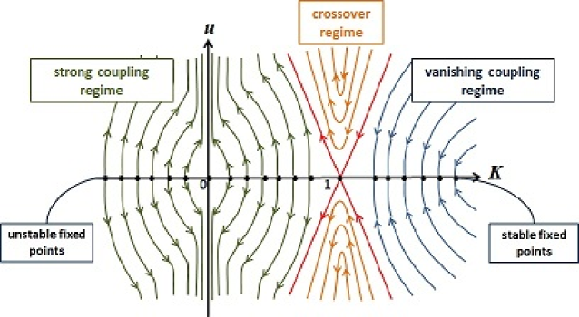
Figure 1: Kosterlitz-Thouless phase diagram for the sine-Gordon model.

IV.2 Gap

In both the strong coupling and the crossover regimes the flows are towards large $|u|$. At some critical scale in these flows, call it $l_{c}$, the interaction becomes too strong, driving a phase transition in the system. Thus, at $l_{c}$, the system loses scale invariance and the R.G. statement is no longer valid. Based on the perturbative nature of the R.G. procedure, a reasonable estimate for $l_{c}$ is the scale at which the flow of $|u|$ reaches unity. The system’s critical correlation length $\xi_{c}$ can be assessed through the expression: $\xi_{c}\propto\exp(l_{c})$.

Since the gap $\Delta\propto\xi_{c}^{-1}$,

$$\Delta=\exp(-\,l_{c})$$

gives an estimate for the gap (except for a multiplicative energy factor) that opens up in a system that starts at $|u_{0}|<1$ and flows to the large $|u|$-regime.

Our task is to determine the value of $l_{c}$, and thus of $\Delta$, as a function of the sine-Gordon bare parameters $K_{0}$ and $|u_{0}|<1$. A first approximation is to consider the perturbative R.G. only up to first order in the coupling constant $g$. At this order, we can straightforwardly integrate the flow equation for $u$ and determine $l_{c}$.

Keeping corrections only up to first order in $g$ would have led to simplified flow equations of the form:

$$\left\{\begin{array}[]{ll}\frac{du}{dl}=2u(1-K)\\ \frac{dK}{dl}=0\\ \end{array}\right.$$ (63)

as can be seen directly from Eqs. (51) and (52) by taking $u^{2}\rightarrow 0$.

Since now $K=K_{0}$ is a constant parameter, we can write:

$$\int_{u_{0}}^{u}\frac{du^{\prime}}{u^{\prime}}=2(1-K_{0})\int_{l_{0}}^{l}dl^{\prime}$$

$$u(l)=u_{0}\exp[2(1-K_{0})(l-l_{0})]$$

We see that, for $K_{0}<1$, $|u|$ increases boundlessly, while for $K_{0}>1$, $|u|$ decreases until it reaches the line of fixed points $u=0$. Note that first order perturbative R.G. cannot capture crossover paths. In particular, $K=1$ represents a line of fixed points at this level of approximation. Just to illustrate, the sine-Gordon model phase diagram produced by first order perturbative R.G. looks as in Fig. 2.

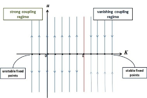
Figure 2: Phase diagram for the sine-Gordon model produced by first order perturbative R.G.

Coming back to the gap, for $K_{0}<1$ and $|u_{0}|<1$ we can write:

$$1=|u_{0}|\exp[2(1-K_{0})(l_{c}-l_{0})]$$

$$l_{c}=l_{0}+\ln(\,|u_{0}|^{1/2(K_{0}-1)}\,)$$

Therefore, in first order approximation:

$$\Delta=\Delta(K_{0},u_{0})=\left\{\begin{array}[]{ll}c_{0}|u_{0}|^{1/2(1-K_{0})}\qquad K_{0}\leq 1\,(and\,|u_{0}|<1)\\ 0\qquad\qquad\qquad\quad K_{0}\geq 1\\ \end{array}\right.$$ (66)

As shown in Fig. 3, for a given $|u_{0}|<1$, the gap decreases with $K_{0}$ (since $|u_{0}|<1$) until it reaches zero at the critical value $K_{0}^{c}=1$. On the other hand, given $K_{0}<1$, the gap increases with $|u_{0}|$ until it reaches its maximum value of $c_{0}=\exp(-l_{0})$ corresponding to $|u_{0}|=1$. This behavior of the gap with $K_{0}$ and $|u_{0}|$ is an expression of the fact that the critical correlation length decreases as one goes deeper into the strong coupling regime, i.e. as $|u_{0}|$ increases and $K_{0}$ decreases.

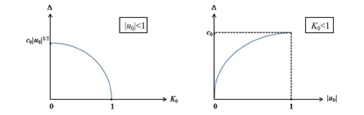
Figure 3: First order gap as a function of $K_{0}$ (left) and $|u_{0}|$ (right).

The line $K=1$ in Fig. 2 defines the boundary between the gapless (vanishing coupling regime) and gapped (strong coupling regime) regions of the phase diagram. The system can undergo a phase transition between the gapless and gapped phases by varying the parameter $K_{0}$ across the line $K=1$.

A first correction to the first order gap of Eq. (66) and Fig. 3 can be achieved by expanding the gapped region into the crossover regime of Fig. 1 (where marginal paths may start at the region $K>1$ but ultimately flow into the large $|u|$ regime). This correction should take into account that the boarder line in the K-T phase diagram is no longer given by $K=1$, but by $K=1\pm u/\sqrt{2}$, where the upper sign stands for $u>0$ while the lower one is for $u<0$.

Based on this and guided by the first-order results of Fig. 3, we can draw a qualitative picture for the gap produced by second-order perturbative R.G. such as depicted in Fig 4.

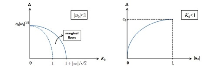
Figure 4: Qualitative picture for the second-order gap as a function of $K_{0}$ (left) and $|u_{0}|$ (right).

For a given $|u_{0}|<1$, the gap decreases with $K_{0}$ until it reaches zero at the critical value $K_{0}^{c}=1+|u_{0}|/\sqrt{2}$. The dashed line on the graph represents the gap as given by first order R.G. The region between the two curves accounts for the contribution of marginal paths to the gap opening. As indicated by the second Eq. (51), for small $K_{0}$, the parameter $K$ remains almost constant along the second order R.G. flow. In other words, close to the line $K=0$, the second order flow is essentially vertical like in first order. Therefore, for small $K_{0}$, the first- and second-order approximations should give roughly the same results for the gap, as shown in Fig. 4. As $K_{0}$ increases, the first and second-order gaps depart from each other to die in different critical points.

Now, given $K_{0}<1$, the dependance of the gap on $|u_{0}|$ should be similar to that of the first order approximation. It is not possible to apply a similar qualitative reasoning for the $K_{0}>1$ region because flows starting there have a non-trivial marginal behavior. In particular, since the marginal flows are “longer”, the critical scale $l_{c}$ (at which a gap would open up) might exceed the system’s cutoff and, in practice, the phase transition might not be realizable. The important point anyway is that, deep inside the strong coupling sector of the K-T phase diagram where the gap is more relevant (larger), $\Delta=c_{0}|u_{0}|^{1/2(1-K_{0})}$ remains a good quantitative estimate.

V Applications in Condensed Matter Physics

The main motivation of the sine-Gordon model to condensed matter physics is that the model is the bosonized version of the fermionic g-ology or Hubbard models for one-dimensional interacting electron systems (the Luttinger liquids). In this context, the sine-Gordon bare parameters $u_{0}$, $K_{0}$ and the non-renormalized velocity $v$ are connected to the original microscopic couplings defined for the fermionic models. A comprehensive review on bosonization methods can be found in the book “Quantum Physics in One Dimension”, by T. Giamarchi Giammarchi .

V.1 The g-ology model

The sine-Gordon bare parameters $\tilde{g}_{0}$, $K_{0}$ and $v$ are related to the 1D g-ology model’s microscopic couplings according to the following expressions Giammarchi1

$$\tilde{g}_{0}\rightarrow\tilde{g}_{0\nu}=\left\{\begin{array}[]{ll}0\quad\nu=c\\ \frac{-2g_{1\perp}}{(2\pi\alpha)^{2}}\quad\nu=s\\ \end{array}\right.$$ (69)

$$K_{0}\rightarrow K_{0\nu}=\left[\frac{1+y_{4\nu}/2+y_{\nu}/2}{1+y_{4\nu}/2-y_{\nu}/2}\right]^{1/2}$$ (70)

$$v\rightarrow v_{\nu}=v_{F}[(1+y_{4\nu}/2)^{2}-(y_{\nu}/2)^{2}]^{1/2}$$ (71)

where

$$y_{\nu}\equiv\frac{g_{\nu}}{\pi v_{F}}$$ (72)

$$g_{\nu}=g_{1\parallel}-g_{2\parallel}\mp g_{2\perp}$$ (73)

$$g_{4\nu}=g_{4\parallel}\pm g_{4\perp}$$ (74)

and the sub-indexes $\nu=c,s$ refer, respectively, to the charge and spin separated sectors of the full bosonized hamiltonian. In Eqs. (73) and (74), the upper signs refer to $c$ and the lower ones to $s$.

In the standard g-ology notation, the coupling $g_{4}$ corresponds to forward scattering between electrons of equal chirality while $g_{2}$ and $g_{1}$ correspond, respectively, to forward and backscattering between electrons of different chiralities. Now, the intensity of each such $g$-scattering may depend on whether the spins of the two interacting electrons are parallel ($g_{\parallel}$) or anti-parallel ($g_{\perp}$, in lack of a better notation). Note that for spinless fermions $g_{2}$ and $g_{1}$ processes are identical since one can exchange the outgoing indiscernible particles. But once the spin comes in the picture, these two process become intrinsically different and contribute to the bosonized theory in different ways, as can be seen from the above equations.

In the general case, when writing models for interacting electrons one is concerned with the standard Coulomb repulsion between the particles. In the present context, this translates into positive $g$-couplings for all processes. However, electrons sometimes can interact in an attractive way (as for example, through a phonon mediated coupling). This possibility is taken into account by allowing for (some) processes with negative g-couplings.

From Eqs. (69)-(74), we see that the Luttinger liquid separates into a charge sector described by a model of free bosons with velocity $v_{c}$ and a spin sector that maps into a bosonic sine-Gordon model with parameters $v_{s}$, $\tilde{g}_{0s}$ and $K_{0s}$. Since $v_{c}\neq v_{s}$ charge and spins excitations travel independently in the system.

From the point of view of the original electronic system, the massless charge sector represents electrons in a metallic phase. The behavior of the spin sector is not as simple but can be understood in the context of the sine-Gordon model phase diagram with bare parameters determined by Eqs. (69)-(74). This phase diagram is depicted in Fig. 5 below.

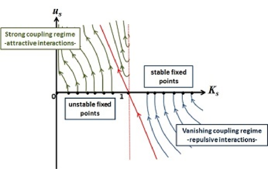
Figure 5: Phase diagram for the spin sector of the g-ology model.

First of all, note that Eq. (70) excludes the $(K<0)$-half of the full K-T phase diagram. In fact, from Eq. (52), a negative $K$ corresponds to an imaginary $\beta$ which, in turn, leads to a hyperbolic cosine in Eq. (1). Although this is certainly a mathematical possibility, it is not the case of physical interest.

Secondly, Eqs. (70)-(73) imply that: $K_{0s}>1$ if $g_{1\parallel}>0$ (for $g_{2}$-processes of comparable intensity), i.e. if $\tilde{g}_{0s}<0$ (assuming that $g_{1\parallel}$ and $g_{1\perp}$ have the same sign), and vice-versa. Therefore, for a repulsive $g_{1}$-interaction, the only physically meaningful region of the full K-T phase diagram is the one bounded above by the line $u_{s}=0$ and to the left by the line $K_{s}=1$. On the other hand, an attractive $g_{1}$-interaction is described by the region bounded below by the line $u_{s}=0$ and to the right by the line $K_{s}=1$ (and to the left by $K_{s}=0$).

Finally, half of the upper crossover regime of the full K-T phase diagram was incorporated to the strong coupling regime since, along the remaining part of the (now relevant) flows, $u_{s}$ increases monotonically. The lower crossover regime, which would have to be “artificially” interrupted at the $K_{s}=1$ line, can be excluded all over based on the argument of weak interactions, i.e. small $|u_{0s}|$.

The conclusions that can be gleaned from the phase diagram can be summarized as follows: Repulsive backscattering processes in 1D electronic systems are irrelevant and the resulting gapless spin excitations behave, in effect, as a collection of free bosons that propagate with velocity $v_{s}$ given by Eqs. (71)-(74). Attractive backscattering processes flow to the regime of strong interactions, i.e. are relevant, causing the opening of a gap in the system’s spin sector. A gapped spin excitation means that the spin $\varphi_{s}$-field gets trapped at a minima of the cosine and orders, breaking rotational symmetry . Assuming that the nature of electronic interactions, i.e. repulsive or attractive, is a definite property of a given system, then it is not possible to drive a phase transition by varying the pair $(K_{0s},u_{0s})$ across the point $(1,0)$.

V.2 The g-ology model at commensurate fillings - umklapp processes

In 1D electron systems with commensurate fillings there is a fourth type of interaction known as umpklapp. The correspondent coupling constant is termed $g_{3}$ in the g-ology dictionary. The most known is the case of half-filling that corresponds to scattering of two left movers to the other side of the Fermi level through a momentum transfer of $4k_{F}$ from the lattice. For quarter-filling, an umklapp will be produced by a similar scattering involving now four particles with a momentum transfer of $8k_{F}$.

In any case, given that the system is at a commensurate filling, the bare parameter $\tilde{g}_{0c}$ of Eq. (69) is no longer zero and is associated with a cosine perturbation of the type

$$+\tilde{g}_{0c}\cos(n.\sqrt{8\pi K_{0c}}\varphi-\delta x)$$ (75)

where

$$\tilde{g}_{0c}=\tilde{g}_{0c}^{n}=\frac{2g_{3,n}}{(2\pi\alpha)^{2}},$$ (76)

$n$ is the order of the commensurability (which affects the amplitude and the wave length of the cosine potential) where $n=1$ corresponds to half-filling, $n=2$ to quarter-filling, etc; and the parameter $\delta$ measures the deviation (doping) from the commensurate filling.

The perturbation will oscillate fast due to the phase shift $\delta x$ and its space integral will vanish unless $\delta x\rightarrow 0$. In other words, away from a commensurate filling (finite $\delta$), the umklapp is absent and we recover the previous picture of free bosonic charge excitations. But at a commensurate filling ($\delta=0$), the Luttinger liquid separates into two independent sine-Gordon models: one for the charge sector with parameters $v_{c}$, $\tilde{g}_{0c}$ and $\bar{K}_{0c}=n^{2}K_{0c}$ and one for the spin sector with parameters $v_{s}$, $\tilde{g}_{0s}$ and $K_{0s}$ (with $v_{\nu}$, $\tilde{g}_{0\nu}$ and $K_{0\nu}$ given by eqs. (69)-(76)).

Fig. 6 shows the phase diagram for the charge sector of the $g$-ology model at half-filling ($n=1$), assuming a positive umklapp coupling $g_{3,n}$. For the charge sector, Eqs. (70)-(73) imply that: $K_{0c}>1$ if $g_{1\parallel}>g_{2\parallel}+g_{2\perp}$, with no implication on the value of $\tilde{g}_{0c}$ (that is proportional to $g_{3,n}$ and, thus, positive). The previous condition leads to a number of possible scenarios. For repulsive interactions, it is verified when backscattering (between electrons having parallel spins) is more than twice as intense as forward scattering. The opposite holds for attractive interactions. If backscattering is repulsive and forward scattering is attractive, the condition is always verified. In the opposite scenario, the condition is never verified. In general, it is possible to drive a phase transition in the charge sector of a 1D commensurate electronic system by tuning the strength of the interactions so that the pair $(K_{0c},u_{0c})$ moves across the separatrix $K_{c}=1+u_{c}/\sqrt{2}$. In the vanishing coupling regime, the umklapp is irrelevant, charge excitations are gapless and the system is a metal. In the strong coupling regime, the umklapp becomes relevant, the charge excitations develop a gap and the system turns into an insulator. In the crossover regime, the umklapp is marginal.

Another way to drive a metal-insulator phase transition in a 1D electronic system is by tuning the filling. Given a fixed $(K_{0c},u_{0c})$ located in the strong coupling regime, the system can undergo a metal-insulator phase transition by varying $\delta$, i.e. the commensurability parameter. This is a phase transition of incommensurate-commensurate type, also known as Mott-transition.

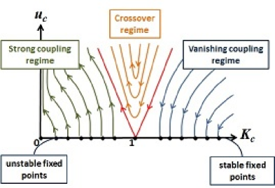
Figure 6: Phase diagram for the charge sector of the g-ology model at half-filling.

V.3 The Hubbard model

The sine-Gordon bare parameters $\tilde{g}_{0}$, $K_{0}$ and $v$ are related to the Hubbard model’s microscopic couplings through the equationsGiammarchi2

$$\tilde{g}_{0}\rightarrow\tilde{g}_{0\nu}=\left\{\begin{array}[]{ll}0\quad\nu=c\\ \frac{-2U}{(2\pi\alpha)^{2}}\quad\nu=s\\ \end{array}\right.$$ (79)

$$vK_{0}\rightarrow v_{\nu}K_{0\nu}=v_{F}$$ (80)

$$\frac{v}{K_{0}}\rightarrow\frac{v_{\nu}}{K_{0\nu}}=v_{F}\left(1\pm\frac{U}{\pi v_{F}}\right)$$ (81)

where, as before, $\nu=c,s$ and the upper sign refers to $c$ and the lower one to $s$. In the Hubbard model, the coupling $U$ represents an on-site interaction of $g_{1}$ nature with the extra restriction that, since the interaction is local, it can only take place between electrons with opposite spins (due to the Pauli principle). The Hubbard model can be seem as a simplification on the g-ology model.

From Eqs. (80) and (81) and the fact that the $K$-parameter is positive, $K_{0s}$ writes in terms of $U$ as:

$$K_{0s}=\frac{1}{\sqrt{1-\frac{U}{\pi v_{F}}}}$$ (82)

Also here the Luttinger liquid separates into independent charge and spin excitations described, respectively, by a free model and a sine-Gordon model with their respective parameters. From Eq. (82), $U>0\Rightarrow K_{0s}>1$ and vice-versa. Therefore, for a system with a repulsive and weak enough Hubbard interaction, the pair of bare parameters $(K_{0s},u_{0s})$ lies inside the $u_{s}<0$ vanishing coupling, irrelevant, regime of the full K-T phase diagram. In this case, only the gapless phase is accessible for the spin system which consists of free bosonic excitations. Meanwhile, for an attractive $U$, the pair of bare parameters $(K_{0s},u_{0s})$ will fall into either the $u_{s}>0$ strong coupling regime or in the left half of the crossover regime where the interaction becomes relevant. In either cases, the spin sector develops a gap and the spin field orders. The spin sector’s phase diagram is the same as in Fig. 5 obtained in the context of for the $g$-ology model. Here, again, we do not expect a phase transition between the gapless and the gapped phases of the spin excitations developing in a metal where the nature of the Hubbard on-site interaction is either repulsive or attractive.

If the system is at half-filling, the charge sector develops an umklapp interaction of the form

$$+\tilde{g}_{0c}\cos(\sqrt{8\pi K_{0c}}\varphi-\delta x)$$ (83)

where in the Hubbard model language:

$$\tilde{g}_{0c}=\frac{2U}{(2\pi\alpha)^{2}},$$ (84)

For commensurate fillings other than $1/2$, the umklapp interaction assumes similar expressions.

From Eqs. (80) and (81), $K_{0c}$ is given in terms of $U$ as:

$$K_{0c}=\frac{1}{\sqrt{1+\frac{U}{\pi v_{F}}}}$$ (85)

Thus, at commensurate fillings, the Luttinger liquid separates into two independent sine-Gordon models: one for the charge and one for the spin sector with their correspondent parameters. Fig. 7 shows the phase diagram for the charge sector of the Hubbard model at half-filling.

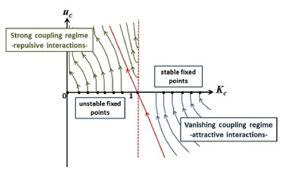
Figure 7: Phase diagram for the charge sector of the Hubbard model at half-filling.

From Eq. (85), $U>0\Rightarrow K_{0c}<1$ and vice-versa. Therefore, for a repulsive interaction, the pair of bare parameters $(K_{0c},u_{0c})$ falls inside either the $u_{c}>0$ strong coupling regime or in the left half of the crossover regime. In both situations the interaction is relevant and the system opens up a gap, becoming an insulator. On the other hand, a weak enough attractive interaction puts $(K_{0c},u_{0c})$ inside the $u_{c}<0$ vanishing coupling regime where the interaction is irrelevant. In this regime, the gapless charge excitations remain in the metallic phase. As before, one cannot drive a metal-insulator phase transition between the repulsive and attractive portions of the phase diagram in a system where the interactions have a definite nature.

In summary, the Hubbard model describes the following types of 1D systems of interacting electrons: Away from commensurability, the system is a metal described by gapless charge excitations and, if the Hubbard interaction is repulsive, gapless spin excitations that preserve rotational symmetry, or gapped and symmetry breaking spin excitations if the interaction is attractive. For commensurate fillings, the system will be an insulator formed of gapped charge excitations and gapless spin excitations for a repulsive interaction, while an attractive interaction leads to a metal with gapless charge excitations and gapped spin excitations.

References

- (1) The question regarding the failure of Fermi liquid theory in was formalized for the first time in 1950 by Tomonaga. He proposed that the fermionic excitations in one dimension should be understood as “quantized sound waves”, that is phonon-like bosonic excitations. In 1963, Luttinger extended this idea and wrote down a model for which he obtained an incorrect solution. The correct solution would come with the work of Mattis and Lieb, in 1965. The term ‘Luttinger liquid’ was coined by Haldane only in 1981 in a work where he proposed a physical interpretation for the bosonic collective modes of single-particle excitations of fermions in .
- (2) M. Karowski, H.J. Thun, Nucl. Phys. B130, 295 (1977).
- (3) A.B. Zamolodchikov, Pisma Zh. Eksp. Teor. Fiz. 25, 499 (1977); Commun. Math. Phys. 55 183 (1077).
- (4) L.T. Faddeev, E.K. Sklyanin, L.A. Takhtajan, Theor. Math. Phys. 40, 688 (1980).
- (5) V.E. Korepin, Commun. Math. Phys. 76, 165 (1980).
- (6) H. Babujian, A. Fring, M. Karowski, A. Zapletal, Nucl. Phys. B538, 535 (1999); H. Babujian, M. Karowski, Nucl. Phys. B620, 407 (2002); H. Babujian, M. Karowski, J. Phys. A35, 9081 (2002).
- (7) C. Destri, H.J. De Vega, Phys. Rev. Lett. 69, 2313 (1992); Nucl. Phys. B504 621 (1997).
- (8) D. Fioravanti, A. Mariottini, E. Quattrini, F. Ravanini, Phys. Lett. B390, 243 (1997).
- (9) G. Feverati, F. Ravanini, G. Takacs, Nucl. Phys. B540, 543 (1999).
- (10) G. Niccoli, J. Teschner, Arxiv:0910.3173v2 (2010).
- (11) T. Giamarchi, Quantum Physics in One Dimension (Oxford University Press, Oxford, 2003).
- (12) See Giamarchi, P. 53, Eqs. (2.105)-(2.106) addapted to the present notation.
- (13) See Giamarchi, P. 202, Eq. (7.9) addapted to the present notation.