Are we there yet? When to stop a Markov chain while generating random graphs

Abstract

Markov chains are a convenient means of generating realizations of networks, since they require little more than a procedure for rewiring edges. If a rewiring procedure exists for generating new graphs with specified statistical properties, then a Markov chain sampler can generate an ensemble of graphs with prescribed characteristics. However, successive graphs in a Markov chain cannot be used when one desires independent draws from the distribution of graphs; the realizations are correlated. Consequently, one runs a Markov chain for $N$ iterations before accepting the realization as an independent sample. In this work, we devise two methods for calculating $N$. They are both based on the binary “time-series” denoting the occurrence/non-occurrence of edge $(u,v)$ between vertices $u$ and $v$ in the Markov chain of graphs generated by the sampler. They differ in their underlying assumptions. We test them on the generation of graphs with a prescribed joint degree distribution. We find the $N\propto|E|$, where $|E|$ is the number of edges in the graph. The two methods are compared by sampling on real, sparse graphs with ${\rm 10^{3}}-{\rm 10^{4}}$ vertices.

1 Introduction

Markov chain Monte Carlo (MCMC) methods are a common means of generating realizations of graphs which share similar characteristics since they require nothing more than a procedure that can generate a new graph by “rewiring” the edges of an existing graph. Much of their use to date has been in generating graphs with a prescribed degree distribution [1, 2, 3, 4]. Other efforts have used MCMC to generate graphs with a prescribed joint degree distribution [5]. MCMC methods require a graph to start the chain; thereafter, the “rewiring” procedure generates new, realizations which preserve certain graph characteristics. The specific characteristic(s) that are preserved depend entirely on the “rewiring” procedure.

MCMC methods for generating graphs has two drawbacks. Initialization bias arises from the fact that the starting graph may not even lie in the population of graphs that we seek to sample, or may be an outlier in that population. The second issue, autocorrelation in equilibrium, arises from the fact that successive samples drawn by the MCMC sampler are correlated and an empirical distribution constructed from them would result in the statistical error (variance) to be 2$\tau_{int}$larger than the distribution constructed using independent samples. Here $\tau_{int}$, the integrated autocorrelation time, is a measure of how slowly correlation in graphical metrics, calculated from an MCMC series, decays; see Sections 2 and 3 in Sokal’s lecture notes [6].

Sokal’s method [6] for deciding the “sufficiency” of samples obtained from MCMC revolve around autocorrelation. The method is general, and was adapted for use with graphs in [5]. Consider an edge $(u,v)$ between labeled vertices $u$ and $v$ in the ensemble of graphs generated by the MCMC chain. Denoting its occurrence/non-occurrence in the chain of graphs by 1/0 gives us a binary time-series $\{Z_{t}\},t=1\ldots T$, with an empirical mean $\mu$. The auto-correlation, with lag $l$, is given by $C(l)=(\{Z_{t}\}-\mu)(\{Z_{t+l}\}-\mu),t=1\ldots T-l$ and the normalized version of it, $\rho(l)=C(l)/C(0)$ can be used to gauge whether the autocorrelation in the time-series is observed to be decreasing. In [5], the authors used this metric, applied to all edges in the graphs that were sampled, to ensure that their MCMC chain was mixed. One can also set, loosely speaking (for details, consult [6]), a minimum threshold $\rho_{min}$, identify the corresponding lag $l_{min}$, and retain every $l_{min}^{th}$ entry in the MCMC chain to serve as independent samples. However, this method has two practical drawbacks. First the autocorrelation analysis has to be performed for all the edges (potentially, $|V|^{2}$ in number) that might appear in the MCMC chain, which quickly becomes prohibitively expensive for large graphs. Secondly, it requires a user input, $\rho_{min}$, which may have an arbitrary effect on graphical properties of the ensemble. These shortcomings motivate our work.

In this paper, we propose two different methods for generating independent graphs using an MCMC method. The first, which we call Method A or “multiple short runs”, determines the number of iterations $N$ an MCMC method has to be run to “forget” the initial graph and minimize the initialization bias. The second approach, Method B or “one long run”, requires $K$ MCMC iterations. This long run is thinned by a factor $k$ (i.e., every $k^{th}$ MCMC iteration is preserved) to generate $K/k$ independent samples. Both methods are intended to be approximate, but simple to evaluate, so that they can be employed in practice to gauge the “sufficiency” of MCMC iterations. The two methods for extracting independent graphs are tested on an MCMC chain with the setup described in [5]. We explore the practical impact of approximations in our methods. We restrict ourselves to undirected graphs with labeled nodes.

In the next section (Sec. 2) we describe the procedure used to “rewire” a graph to create a new graph realization with the same joint degree distribution. In Sec. 3 we describe the two methods for generating independent samples. In Sec. 4, we test the methods on real sparse graphs. We conclude in Sec. 5.

2 A Markov chain algorithm for sampling graphs with a given joint degree distribution

Consider an undirected graph $G=(V,E)$, where $|V|=n$ and $|E|=m$. The degree distribution of the graph is given by the vector $\vec{f}$, where $f(d)$ is the number of vertices of degree $d$. The joint degree distribution list the number of edges incident between vertices of specified degrees. Formally, the $n\times n$ matrix $\mathbf{J}$ denotes the joint degree distribution, where the entry $J(i,j)$ is the number of edges between vertices of degree $i$ and degree $j$. Stanton and Pinar [5] studied the problem of generating and random sampling a graph with a given joint degree distribution. They proposed a greedy algorithm to construct an instance of a graph with a specified (feasible) degree distribution, as well as a Markov chain algorithm to generate random samples of graphs with the same degree distribution.

For the purposes of this paper, we will only focus on the Markov chain algorithm. The rewiring operation that moves us between the nodes of the Markov chain is depicted in Fig. 1. At the first step, one picks an edge $(u_{1},v)$ at random and thereafter, one of the end vertices, e.g., $u_{1}$. We wish to break $(u_{1},v)$ and connect $u_{1}$ and $v$ to others without violating the prescribed joint degree distribution. We, therefore, search for another edge $(u_{2},w)$ where $d_{u_{2}}=d_{u_{1}}$ or $d_{w}=d_{u_{1}}$, where $d_{p}$ denotes the degree of node $p$. WLOG, let $d_{u_{2}}=d_{u_{1}}$. Swapping the edges i.e. creating edges $(u_{1},w)$ and $(u_{2},v)$ while destroying $(u_{1},v)$ and $(u_{2},w)$ leaves the joint degree distribution unchanged while changing the connectivity pattern of the graph. If the resulting graph is simple, the graph is retained by the MCMC chain.

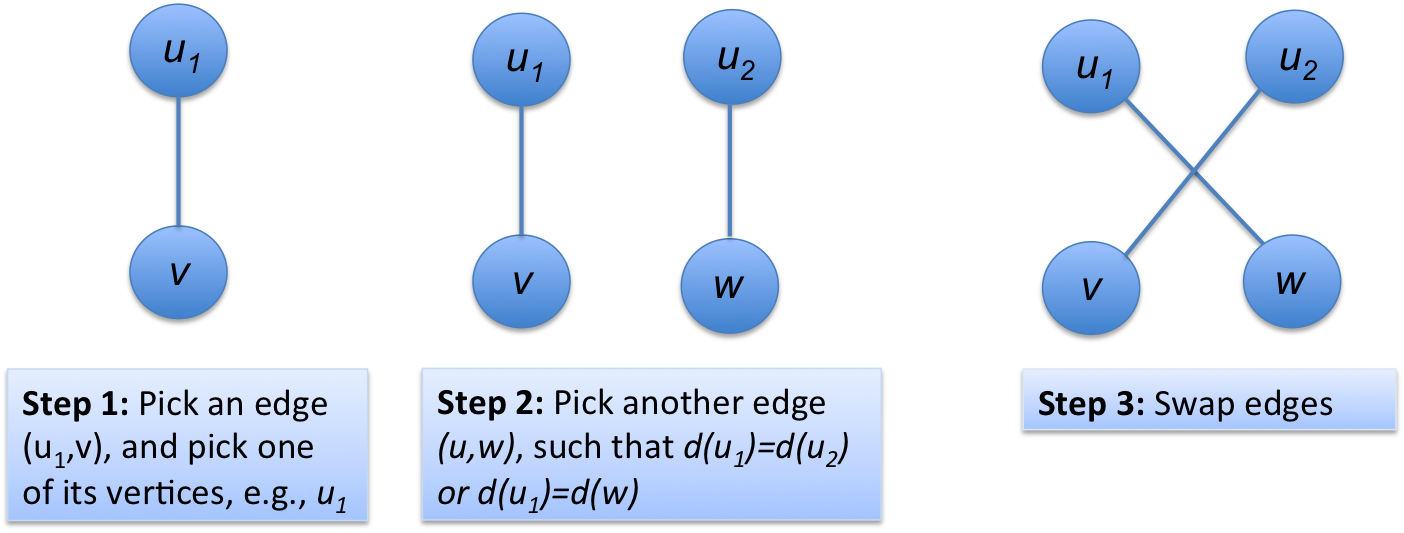
Figure 1: The swapping operation for the Markov chain algorithm.

The procedure results in inter-edge correlation. A particular edge is chosen for swapping, on average, once every $|E|$ Markov chain iterations. In [5], this procedure was used to generate graphs (of moderate sizes, with $|V|\leq 23,000$), using an MCMC sampler. Autocorrelation analysis showed that the Markov chain mixes and the autocorrelation decays with edge-dependent rates. Empirically it was observed that an edge $(u,v)$ de-correlated slowly if $J(d_{u},d_{v})/(f{d_{u}}f{d_{v}})\approx 0.5$. Empirically, it was observed that the autocorrelations of the edges decreased very sharply.

3 Methods for calculating independence

The algorithm in Sec. 2 has two variants - one where the resulting graph may not be simple, and another where the graph was always simple (A graph is simple if it does not have self-loops or parallel edges). For the first variant, earlier work [1] implies that this chain has a polynomial mixing time. The second variant is not even known to have any bounds on the mixing time. As discussed in Sec. 1, one would like to provide a length to run the MCMC that, although not guaranteeing complete mixing, at least gives some confidence that the sampled graph is fairly “random.” To that end, we will we will approximate the behavior of a single edge by a Markov chain. We stress that we do not give a proof, but only a mathematical argument justifying this. Below we present two methods for generating independent graph samples.

3.1 Method A - “multiple short runs”

We refer to this method as Method A or the “multiple short runs” method. We generate $M$ graph samples by running $M$ independent Markov chain for $N$ iterations before accepting the resulting graph. All the chains are run from the same initial graph; however, the state in the random number generator in each of the $M$ MCMC chains are distinct.

Consider a fixed pair of labeled vertices $\{u,v\}$. We will approximate the occurrence of an edge between $(u,v)$ as a two state Markov chain. Note that this is an approximation, since these transitions depend on the remaining graph if $\mathbf{J}$ is to be preserved. Nonetheless, these dependencies appear to be weak. The first coordinate of the matrix is state $0$ (no edge) and the second coordinate is $1$, indicating the existence of an edge. The transition matrix $\mathbf{T}$ for this chain is

$$\mathbf{T}_{i,j}=\left(\begin{array}[]{cc}1-\alpha_{i,j}&\alpha_{i,j}\\ \beta_{i,j}&1-\beta_{i,j}\end{array}\right),$$ (1)

where $i=d_{u}$ and $j=d_{v}$ are the degrees of vertices $u$ and $v$. $\alpha_{i,j}$ and $\beta_{i,j}$ are positive fractions and $(\alpha_{i,j}+\beta_{i,j})\leq 1$. The eigenvalues of the transition matrix are 1 and $1-(\alpha_{i,j}+\beta_{i,j})$. Below, we construct a model for $\alpha_{i,j}$ and $\beta_{i,j}$.

Suppose the state is currently $0$. The state will become $1$ if the edge $(u,v)$ is swapped in. Let the two edges chosen by the algorithm be $e$ and $e^{\prime}$, in that order. The edge $(u,v)$ is swapped in if $e$ contains $u$ and $e^{\prime}$ contains $v$ (or vice versa). Furthermore, the endpoint $u$ must be chosen, and the other end of $e^{\prime}$ must have degree $d_{u}$. The probability that $e$ contains $u$ and $u$ is chosen as an endpoint is exactly $d_{u}/2m$. The probability we choose the edge $e^{\prime}$ that is incident to $v$ depends on the number of neighbors of $v$ whose degree is $d_{u}$. Clearly, this depends on the graph structure (leading in a non-Markov probability of this transition). We heuristically guess this number based on the joint degree distribution. The number of edges from degree $d_{u}$ to degree $d_{v}$ vertices is $\mathbf{J}(d_{u},d_{v})$. Of these, the average number of edges incident to a fixed vertex of degree $d_{v}$ is $\mathbf{J}(d_{u},d_{v})/f_{v}$. We shall approximate the number of edges incident to $v$ with the other endpoint of degree $d_{u}$ by this quantity. The total probability is

$$\frac{d_{u}}{2m}\times\frac{\mathbf{J}(d_{u},d_{v})}{mf(d_{v})}=\frac{d_{u}\mathbf{J}(d_{u},d_{v})}{2m^{2}f(d_{v})}$$

The edge $(u,v)$ is also swapped in when the reverse happens (so we choose $v$ as an endpoint, and an edge incident to $u$ with the other endpoint of degree $d_{v}$). The total transition probability from $0$ to $1$ is approximated by

$$\alpha_{i,j}=\frac{d_{u}\mathbf{J}(d_{u},d_{v})}{2m^{2}f(d_{v})}+\frac{d_{v}\mathbf{J}(d_{u},d_{v})}{2m^{2}f(d_{u})}=\frac{\mathbf{J}(d_{u},d_{v})}{2m^{2}}\left(\frac{d_{u}}{f(d_{v})}+\frac{d_{v}}{f(d_{u})}\right)$$ (2)

We now address the transition from $1$ to $0$. Suppose $(u,v)$ is currently an edge. If the first edge $e$ is chosen to be $(u,v)$, then $(u,v)$ will definitely be swapped out. The probability of this is $1/m$. If the random endpoint chosen has degree $d_{u}$ (and is not $u$), then we might choose $e^{\prime}$ to be $(u,v)$. The total probability of this is

$$\frac{(f(d_{u})-1)d_{u}}{2m}\times\frac{1}{m}=\frac{(f(d_{u})-1)d_{u}}{2m^{2}}$$

The roles of $u$ and $v$ can also be reversed, so the total transition probability from $1$ to $0$ is

$$\frac{f(d_{u})d_{u}+f(d_{v})d_{v}-d_{u}-d_{v}}{2m^{2}}$$

and so

$$\beta_{i,j}=\frac{1}{m}+\frac{f(d_{u})d_{u}+f(d_{v})d_{v}-d_{u}-d_{v}}{2m^{2}}$$ (3)

We proceed to determining the number of iterations $N$ to run the Markov chain. We start the Markov chain ${\mathcal{M}}$   with an initial distribution ${\mathbf{v}}$ (which is either $(0,1)$ or $(1,0)$). ${\mathcal{M}}$, which is represented by $\mathbf{T}_{i,j}$ (Eq. 1), is run for $N=ln(1/\epsilon)/(\alpha+\beta)$ iterations, $\epsilon>0$. We have dropped the subscripts $i$ and $j$, since it is implied that this model is being derived for an edge $(u,v)$ with vertices of degrees $i$ and $j$. After $N$ steps, we realize a 2-state distribution ${\mathbf{p}}=(p_{0},p_{1})$, which is different from the stationary distribution be ${\mathbf{u}}=(u_{0},u_{1})$.

Denote the unit 2-norm eigenvectors of $\mathbf{T}$, corresponding to the eigenvalues 1 and $1-(\alpha+\beta)$, as ${\mathbf{e}}_{1}$ and ${\mathbf{e}}_{2}$. The initial state can be expressed as ${\mathbf{v}}=c_{1}{\mathbf{e}}_{1}+c_{2}{\mathbf{e}}_{2}$. After $N$ applications of the transition matrix we get

$${\mathbf{p}}=\mathbf{T}^{N}{\mathbf{v}}=c_{1}\mathbf{T}^{N}{\mathbf{e}}_{1}+c_{2}\mathbf{T}^{N}{\mathbf{e}}_{2}=c_{1}{\mathbf{e}}_{1}+c_{2}\left(1-(\alpha+\beta)\right)^{N}{\mathbf{e}}_{2}.$$

Since $(1-\{\alpha+\beta\})<1$, the second term decays with $N$ and $c_{1}{\mathbf{e}}_{1}$ is the stationary distribution. We can bound the decaying term as

$$\|(1-(\alpha+\beta))^{N}c_{2}{\mathbf{e}}_{2}\|_{2}=(1-(\alpha+\beta))^{\ln(1/\epsilon)/(\alpha+\beta)}c_{2}\|{\mathbf{e}}_{2}\|_{2}\leq\exp(-\ln(1/\epsilon))=\epsilon$$

Hence, $\|{\mathbf{p}}-{\mathbf{u}}\|_{2}\leq\epsilon$, and so each $|p_{i}-u_{i}|$ is at most $\epsilon$. Further, from Eq. 2 and 3, we see that $\alpha+\beta\geq 1/m$ (to leading order) and consequently

$$N=\frac{\ln(1/\epsilon)}{\alpha+\beta}\leq m\ln(1/\epsilon)=|E|\ln\left(\frac{1}{\epsilon}\right).$$ (4)

3.2 Method B - “one long run”

We propose a second method, which we refer to as Method B or “one long run”, for generating independent graphs. The procedure involves running a Markov chain for a large number of steps $K$ and thinning it by a factor $k$ i.e., preserving every $k^{th}$ instance of the chain. Comparing with the development in Sec. 3.1, we expect $k\sim N$.

Similar to Method A (Sec. 3.1), this method too begins with the binary time-series of edge occurrence $\{Z_{t}\}$. As observed in  [5], the autocorrelation in $\{Z_{t}\}$ decays for all edges. Consequently it is possible to successively thin the chain $\{Z_{t}\}$ (i.e., retain every $k^{th}$ element to obtain $\{Z^{k}_{t}\}$, the $k-$thinned chain) and compare the likelihoods that the chains were generated by (1) independent sampling or (2) by a first-order Markov process. When sufficiently thinned, the independent sampling model is expected to fit the data better. Using this as the stopping criterion removes an ambiguity (user-specified tolerances). We will employ a method based on comparison of log-likelihoods of model fit. We derive these expressions below. While this technique has been applied in other domains [7, 8], but this paper is the first application of this technique to graphs.

Consider the chain $\{Z^{k}_{t}\}$. We count the number, $x_{ij}$, of the $(i,j),i,j\in(0,1)$ transitions in it. $x_{ij}$ are used to populate $X$, a $2\times 2$ contingency table. Dividing each entry by the length of thinned chain $K/k-1$ provides us with the empirical probabilities $p_{ij}$ of observing an $(i,j)$ transition in $\{Z^{k}_{t}\}$. Let $\widehat{p_{ij}}$ and $\widehat{x_{ij}}=(K/k-1)\widehat{p_{ij}}$ be the predictions of the probabilities and expected values of the table entries provided by a model. In such a case, the goodness-of-fit of the model is provided by a likelihood ratio statistic (called the $G^{2}$-statistic; Chapter 4.2 in [9]) and a Bayesian Information Criterion (BIC) score

$$G^{2}=-2\sum_{i=0}^{i=1}\sum_{i=0}^{i=1}x_{ij}\log\left(\frac{\widehat{x_{ij}}}{x_{ij}}\right),\mbox{\hskip 28.45274pt}BIC=G^{2}+n\log\left(\frac{K}{k}-1,\right)$$ (5)

where $n$ is the number of parameters in the model used to fit the table data. Typically log-linear models are used for the purpose (Chapter 2.2.3 in [9]); the log-linear models for table entries generated by independent sampling and a first-order Markov process are

$$\log(p_{ij}^{(I)})=u^{(I)}+u^{(I)}_{1,(i)}+u^{(I)}_{2,(j)}\mbox{\hskip 2.84526pt and \hskip 2.84526pt}\log(p_{ij}^{(M)})=u^{(M)}+u^{(M)}_{1,(i)}+u^{(M)}_{2,(j)}+u^{(M)}_{12,(ij)},$$ (6)

where superscripts $I,M$ indicate an independent and Markov process respectively. The maximum likelihood estimates (MLE) of the model parameters ($u^{(W)}_{b,(c)}$) are available in closed form (Chapter 3.1.1 in [9]). They lead to the model predictions below

$$\widehat{x_{ij}^{I}}=\frac{(x_{i+})(x_{+j})}{x_{++}}\mbox{\hskip 5.69054pt and \hskip 5.69054pt}\widehat{x_{ij}^{M}}=x_{ij},$$ (7)

where $x_{i+}$ and $x_{+j}$ are the sums of the table entries in row $i$ and column $j$ respectively. $x_{++}$ is the sum of all entries (i.e., $K/k-1$, the number of transitions observed in $\{Z^{k}_{t}\}$, or the total number of data points). We compare the fits of the two models thus:

$$\Delta BIC=BIC^{(I)}-BIC^{(M)}=-2\sum_{i=0}^{i=1}\sum_{i=0}^{i=1}x_{ij}\log\left(\frac{\widehat{x_{ij}^{(I)}}}{x_{ij}}\right)-\log\left(\frac{K}{k}-1\right).$$ (8)

Above, we have substituted $\widehat{x_{ij}^{(M)}}=x_{ij}$ and the fact that the log-linear model for a Markov process has one more parameter than the independent sampler model. Large BIC values indicate a bad fit. A negative $\Delta BIC$ indicates that an independent model fits better than a Markov model.

The procedure for identifying a suitable thinning factor $k$ then reduces to progressively thinning $\{Z^{k}_{t}\}$ till $\Delta BIC$ in Eq. 8 becomes negative. We search for $k$ in powers of 2. The value of $k$ so obtained varies between edges and conservatively, we take the largest $k,k_{*}$. However, this may be too conservative, i.e, $k_{*}\gg N$, if a few edges are seen to display a slow autocorrelation decay. If we are interested in certain global metrics for graph e.g., maximum eigenvalue etc, a few correlated edges are unlikely to have any substantial effect. Thus, one may be able to thin with a $k\sim N\ll k_{*}$. We will test this empirically in Sec. 4.

4 Tests with real graphs

In this section we first explore the impact of $\epsilon$ (as defined in Sec. 3.1) on the ensemble of graphs generated by a Markov chain, and choose a $\epsilon$ for further use. Thereafter we compare the graphs generated by the Methods A and B (Sec. 3.1 and Sec. 3.2) and gauge the impact of choosing a thinning factor $k<k_{*}$. All tests are done with four real networks - the neural network of C. Elegans [10] (referred to as “C. Elegans”), the power grid of the Western states of US [10] (called “Power”), co-authorship graph of network science researchers [11] (referred to as “Netscience”) and a 75,000 vertex graph of the social network at Epinions.com [12] (“Epinions”). Their details are in Table 1. The first three were obtained from [13] while the fourth was downloaded from [14]. All the graphs were converted to undirected graphs by symmetrizing the edges.

We start the Markov chain using the real networks listed in Table 1. When comparing ensembles of graphs, we will use the (distributions of) global clustering coefficient, number of triangles in the graphs, the graph diameter and the maximum eigenvalue as metrics.

Table 1: Characteristics of the graphs used in this paper. $(|V|,|E|)$ are the numbers of vertices and edges in the graph, $N$ are the number of Markov chain steps used for generating graphs in Sec. 3.1 and $k$ is its equivalent obtained by the method in Sec. 3.2. $K/k_{*}$ are the number of graph samples, obtained by thinning a long run, that were used to generate distributions in the figures.

Graph name	$(|V|,|E|)$	$N/|E|$	$k_{*}/|E|$	$K/k_{*}$
C. Elegans	(297, 4296)	10	13	3582
Netscience	(1461, 5484)	10	49	737
Power	(4941, 13188)	10	13	1214
Epinions	(75879, 405740)	30	720	various

In Fig. 2 we investigate the impact of $\epsilon$ in Method A (“many short runs”). We generate 1000 samples by running the Markov chain for $1|E|,5|E|,10|E|$ and $15|E|$ Markov chain iterations, corresponding to $\epsilon=0.37,6.7\times 10^{-3},4.5\times 10^{-5}$ and $3.06\times 10^{-7}$. In Fig. 2, we plot the distributions for the first three graphs (in Table 1) and find that for all three, $\epsilon<5.0\times 10^{-3}$ lead to distributions which are very close. We will proceed with $\epsilon=4.5\times 10^{-5}$ i.e., when we use Method A, we will mix the Markov chain $10|E|$ times before extracting a sample.

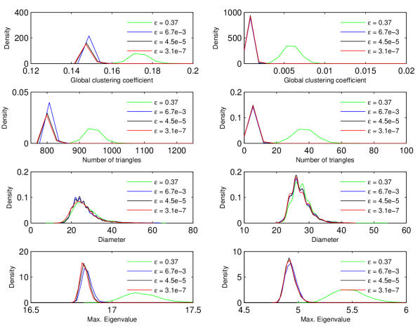
Figure 2: Plots of the distributions of the global clustering coefficient, the number of triangles in the graphs, the graph diameter and the max eigenvalue of the graph Laplacian for “Netscience” (left) and “Power” (right), evaluated after $1|E|,5|E|,10|E|$ and $15|E|$ iterations of the Markov chain (green, blue, black and red lines respectively). The corresponding values of $\epsilon$ are in the legend. We see that the distributions converge at $\epsilon<1.0^{-5}$.

In Table 1 we see that Method B (“one long run”) method often prescribes a thinning factor that is larger than the one obtained using Method A (“multiple short runs”). This large number is often due to the lack of autocorrelation decay in a few edges. We investigate whether such a lack has a significant impact on the graphical metrics that we have chosen. In Fig. 3 we plot distributions of the same metrics for the three graphs. The thinning factors are in Table 1. We see that the distributions are close, i.e., the existence of a few edges whose time-series are still correlated do not impact the metrics of choice. We have repeated these tests with other metrics and the same result holds true.

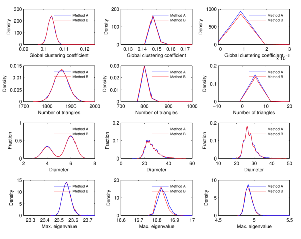
Figure 3: Comparison of the distributions of the global clustering coefficient, the number of triangles in the graphs, the graph diameter and the max eigenvalue of the graph Laplacian for “C. Elegans” (left), “Netscience” (middle) and “Power” (right), evaluated using Methods A (“many short runs”) and B (“one long run”). We see that the distributions are very similar. The kernel density estimation used to generate the distributions sometimes causes nonsensical artifacts e.g., a small, but negative clustering coefficient. For Method A, the Markov chain was run for $10|E|$ iterations. Thinning factors for Method B are in Table 1.

We now address a large graph (Epinions). Since potentially $|V|^{2}$ distinct edges might be realized during a Markov chain, it is infeasible to calculate a thinning factor for all the edges. Consequently, we perform the thinning analysis for only $0.1|E|$ (40,574) edges, chosen randomly from all the distinct edges that are realized by the Markov chain. In Fig. 4 we plot the distribution of $k$ obtained from the 40,574 sampled edges. We see that most of the $k$ lie between $10|E|$ and $100|E|$; edges with thinning factors outside that range are about two orders of magnitude less abundant. It is quite conceivable that there are edges (which were not captured by the sample) that would prescribe an even higher thinning factor. In order to check whether these edges have a significant impact on the distribution of graph metrics, we check their convergence as a function of the thinning factor.

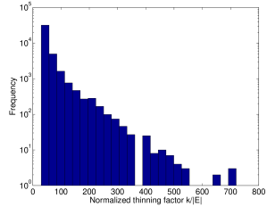
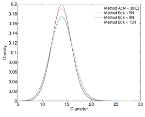
Figure 4: Left: The normalized thinning factor $k/|E|$ for the Epinions graph, as calculated for the 40,574 sampled edges. We see that the most thinning factors are lie in ($10|E|,100|E|$). Right: Plot of the graph diameter and distribution generated using Method A (with $N=30|E|$) and Method B (with $k$ equal to various multiples of $N$). We see that the distributions are very similar.

We generate separate ensembles of graphs. The reference ensemble is generated using Method A, with $N=30|E|$. As seen in Table 1, certain edges will still be correlated ($N=720|E|$ would make them independent). We then use Method B to generate graph ensembles with thinning factors $k/|E|<720$ which are also multiples of $N$. In Fig. 4 (right), the diameter distribution obtained with Method A is compared to that obtained with Method B. While the distributions are very similar, they do display some small differences. This is surprising since $N=30|E|$ indicates a minuscule $\epsilon$. In addition, distributions obtained with $k=5N,9N,$ and $13N$ show some differences between themselves, indicating that the edges that have not become independent have a small, but measurable impact on the graph diameter. Further, the distributions using smaller values of $k$ are marginally wider (have a larger variance), indicating that they were constructed using samples which were not completely independent. However, the differences are minute, and for practical purposes the graph ensemble generated using Method A with $N=30|E|$ is identical to the one generated using Method B, per our chosen metrics. Consequently, despite its approximations, the results in Sec. 3.1 furnish a workable estimate of $N$, if one uses $\epsilon<10^{-5}$. Further, $k_{*}$ is generally too conservative if our aim is to obtain “converged” distributions of certain graph metrics. This arises from a few edges that de-correlate slowly, but have little effect on global graphical metrics due to their rarity.

5 Conclusions

We have developed a method that allows one to generate a set of independent realizations of graphs with a prescribed joint degree distribution. The graphs are generated using an MCMC approach, employing the algorithm described in [5] as the “rewiring” mechanism. The graphs so generated are tightly correlated; our two methods address the question of how one can decorrelate the chain.

The first method, variously called Method A or “multiple short chains”, involves running the Markov chain for $N$ steps before extracting a graph realization; the Markov chain is run repeatedly to generate samples. We developed a model (and a closed-form expression) to estimate $N$ that allows the Markov chain to converge to its stationary distribution before a graph realization is extracted from it. This model assumes that edges are independent. In reality, their behavior is correlated, which leads us to incur small errors.

The second method, variously called Method B or “one long chain”, is a data driven method. It uses the time-series of the occurence/non-occurence of edges in an MCMC run. It does not assume a constant joint degree distribution. It progressively thins the time-series (by retaining every $k^{th}$ element) and fits a first-order Markov and an independent sampling model to the data. The thinning process stops when the independent model has a higher likelihood (strictly, a lower BIC score) than the Markov process. Since this method is data-driven and does not require any user-defined tolerances, we use it to validate Method A. The method is not new, but does not seem to have been used in the generation of independent graphs.

Comparing the two methods, we find that for practical purposes, the ensembles generated using Method A are statistically similar to those obtained with Method B, as gauged by a set of graph metrics. Even at tight tolerance values, a small number of edges in the graphs generated by Method A remain correlated, and the metrics’ distributions are slightly wider. This problem is very small (nearly unmeasureable) in small graphs, but becomes measureable, but still small, for large graphs.

While this work enables the generation of independent graphs, including large ones, it poses a number of questions for further investigation. For example, being able to estimate or bound the difference in the distributions generated by Methods A and B would be helpful. Further, an intelligent way of identifying hard-to-decorrelate edges would reduce the computational burden of checking for the stopping criterion using Method B; currently, we simply use a random set of edges. Finally, it would be interesting if Method A could be extended to the generation of independent graphs when some graph property, other than the joint degree distribution, is held constant. This is currently being studied.

References

- [1] Kannan, R., Tetali, P., Vempala, S.: Simple Markov-chain algorithms for generating bipartite graphs and tournaments. Random Struct. Algorithms 14(4) (1999) 293–308
- [2] Jerrum, M., Sinclair, A.: Fast uniform generation of regular graphs. Theor. Comput. Sci. 73(1) (1990) 91–100
- [3] Jerrum, M., Sinclair, A., Vigoda, E.: A polynomial-time approximation algorithm for the permanent of a matrix with nonnegative entries. J. ACM 51(4) (2004) 671–697
- [4] Gkantsidis, C., Mihail, M., Zegura, E.W.: The Markov chain simulation method for generating connected power law random graphs. ALENEX (2003) 16–25
- [5] Stanton, I., Pinar, A.: Constructing and sampling graphs with a prescribed joint degree distribution using markov chains. ACM Journal of Experimental Algorithmics to appear.
- [6] Sokal, A.: Monte Carlo methods in statistical mechanics: Foundations and new algorithms (1996)
- [7] Raftery, A., Lewis, S.M.: Implementing MCMC. In Gilks, W.R., Richardson, S., Spiegelhalter, D.J., eds.: Markov Chain Monte Carlo in Practice. Chapman and Hall (1996) 115–130
- [8] Raftery, A.E., Lewis, S.M.: How many iterations in the Gibbs sampler? In Bernardo, J.M., Berger, J.O., Dawid, A.P., Smith, A.F.M., eds.: Bayesian Statistics. Volume 4., Oxford University Press (1992) 765–766
- [9] Bishop, Y.M., Fienberg, S.E., Holland, P.W.: Discrete multivariate analysis: Theory and practice. Springer-Verlag, New York, NY (2007)
- [10] Watts, D.J., Strogatz, S.H.: Collective dynamics of ’small-world’ networks. Nature 393 (1998) 440–442
- [11] Newman, M.E.J.: Finding community structure in networks using the eigenvectors of matrices, 036104. Phys. Rev. E 74 (2006)
- [12] Richardson, M., Agrawal, R., Domingos, P.: Trust management for the semantic Web. In Fensel, D., Sycara, K., Mylopoulos, J., eds.: The Semantic Web - ISWC 2003. Volume 2870 of Lecture Notes in Computer Science. Springer Berlin / Heidelberg (2003) 351–368 10.1007/978-3-540-39718-2_23.
- [13] Newman, M.E.J.: Prof. M. E. J. Newman’s collection of graphs at University of Michigan http://www-personal.umich.edu/m̃ejn/netdata/.
- [14] Stanford Network Analysis Platform Collection of Graphs: The Epinions social network from the Stanford Network Analysis Platform collection http://snap.stanford.edu/data/soc-Epinions1.html.