Measurable quantum geometric phase from a rotating single spin

Abstract

We demonstrate that the internal magnetic states of a single nitrogen-vacancy defect, within a rotating diamond crystal, acquire geometric phases. The geometric phase shift is manifest as a relative phase between components of a superposition of magnetic substates. We demonstrate that under reasonable experimental conditions a phase shift of up to four radians could be measured. Such a measurement of the accumulation of a geometric phase, due to macroscopic rotation, would be the first for a single atom-scale quantum system.

The quantum geometric phase is at the core of our understanding of the non-intuitive quantum view of the world, with historical origins going back to the original paper by Aharonov and Bohm Aharonov59 , in 1959. However, while there have been many experimental demonstrations on ensembles of quantum systems, no measurement of a quantum phase on an individual quantum system, undergoing macroscopic rotation, has been performed. In this paper we analyze the appearance of the geometric phase in defects in diamond and show how the measurement of the geometric phase of a single quantum spin, undergoing macroscopic rotation, is now in reach.

In 1984, M.V. Berry developed an elegant and powerful mathematical framework which established the Aharonov-Bohm effect as just one instance of a far more general class of phenomena Berry84 . Berry considered the evolution of a system under a Hamiltonian which is adiabatically changed over time. He showed that the state of such a system acquires a phase which is geometrical in nature. The phase depends only on the system’s path in parameter space, specifically the flux of some gauge field enclosed by that path.

Berry’s work has since been applied to a diversity of phenomena, which can be broadly grouped under the umbrella of geometric phases or topological phases Shapere89 ; Anandan92 . Specific instances of these geometric phases include the following: various analogues of the Aharonov-Bohm effect Aharonov84 ; Casella90 ; He01 ; the rotation of the polarisation of light in twisted optical fibres, which was recognised by Pancharatnam well before Berry’s paper Pancharatnam56 ; the so-called molecular Aharonov-Bohm effect which introduces a gauge field to nuclear degrees of freedom in the Born-Oppenheimer approximation to molecular dynamics Mead79 ; Mead80 ; Jackiw88 ; Mead92 ; and even the dynamics of classical systems such as low Reynolds number hydrodynamics Shapere89a .

Geometric phases have also proved a fruitful avenue of investigation for mathematical physicists due to their rich topological properties and their close connection with gauge theories of quantum fields. Examples include mathematically formulating geometric phases in terms of the holonomy of line bundles Simon83 and directly using the geometric phase to help explain fractional statistics in the quantum Hall effect Arovas84 and the origin of Wess-Zumino terms in theories of quantum chromodynamics Stone86 .

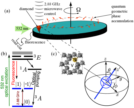
Figure 1: (a) Schematic of system: a diamond crystal containing NV centres, on a spinning table, with the microwave control polarized along the axis of rotation and the $532$ nm optical pulse used for readout. As the NV centre rotates around the axis the $m=\pm 1$ states can accumulate a geometric phase. An example of such phase accumulation is schematically shown for the $m=1$ state with the NV axis in the plane of rotation, i.e. $\theta=\pi/2$. (b) Energy level diagram of the NV center. (c) Geometry of the NV center. Defining the magnetic field direction of the microwave pulses as the $z$-direction, $z^{\prime}$ is the instantaneous direction of the NV axis, defined with respect to the lab-frame, unprimed coordinate system, by $\theta$ and $\phi$.

Despite this wealth of applications and observations, to date, only a few experimental observations of geometric phases due to mechanical rotation have been made Tycko87 ; Appelt94 . These measurements have been on ensembles of ³⁵Cl Tycko87 and ¹³¹Xe Appelt94 nuclear spins. However, no such measurement has been performed on an individual quantum system.

Here we show how this might now be achieved using the quantum properties of a diamond, rotating around an axis, see Fig. 1(a). Such a measurement would represent a significant contribution to the foundations of quantum mechanics. The diamond nitrogen-vacancy (NV) system presents itself as an excellent tool for studying geometric phases. The electron spin is the canonical quantum system and the NV center offers a system in which a single spin can be initialised, coherently controlled, and measured. It is also possible to mechanically move the diamond crystal, and the NV with it, about some cyclical macroscopic trajectory within the spin coherence lifetime. As such this is an ideal system to investigate the accumulation of geometric phase, due to macroscopic rotation, on an individual quantum state.

The NV defect has a spin triplet ground state with a $2.88$ GHz zero-field splitting between the $m=0$ state and the degenerate $m=\pm 1$ inert states [Fig. 1(b)]. Optical excitation with $532$ nm light can pump the defect into the $m=0$ state and allows the population of the ground state to be read, since the $m=0$ state produces more fluorescence than the $m=\pm 1$ states Manson06 ; Steiner10 . The effective Hamiltonian of the ground state, ignoring crystal asymmetries and hyperfine effects, is

$$H=\frac{1}{\hbar}DS_{z^{\prime}}^{2}+\frac{g\mu_{B}}{\hbar}\bm{B}\cdot\bm{S}.$$ (1)

The first term is the zero-field splitting of the NV system itself, where $D$ is the zero-field splitting strength. It is this term which makes the crystal’s orientation crucial. It defines an intrinsic quantisation direction $z^{\prime}$ (we reserve $z$ for the lab-frame coordinate) which lies along the axis connecting the nitrogen atom to its adjacent vacancy [Fig. 1(c)]. The second term is the usual Zeeman splitting interaction with a magnetic field. The magnetic field is $\bm{B}$, and $g\approx 2$ and $\mu_{B}$ are the Landé $g$ factor and the Bohr magneton respectively.

To evaluate the geometric phase for the NV center the instantaneous eigenstates of the Hamiltonian in terms of the adiabatically varied parameters $\theta$ and $\phi$ [see Fig. 1(b)] need to be determined. Writing the zero field splitting Hamiltonian as

$$H_{0}=\frac{1}{\hbar}DS_{z^{\prime}}^{2}=$$

$$D\hbar\left(\begin{array}[]{ccc}\cos^{2}\theta+\frac{\sin^{2}\theta}{2}&\frac{e^{-i\phi}\cos\theta\sin\theta}{\sqrt{2}}&\frac{e^{-2i\phi}\sin^{2}\theta}{2}\\ \frac{e^{i\phi}\cos\theta\sin\theta}{\sqrt{2}}&\sin^{2}\theta&-\frac{e^{-i\phi}\cos\theta\sin\theta}{\sqrt{2}}\\ \frac{e^{2i\phi}\sin^{2}\theta}{2}&-\frac{e^{i\phi}\cos\theta\sin\theta}{\sqrt{2}}&\cos^{2}\theta+\frac{\sin^{2}\theta}{2}\end{array}\right)_{z}$$ (5)

with eigenstates $\psi_{z^{\prime}}^{(m)}$:

$$\psi_{z^{\prime}}^{(1)} = \left(\begin{array}[]{c}\cos^{2}\frac{\theta}{2}\\ \frac{e^{i\phi}}{\sqrt{2}}\sin\theta\\ e^{2i\phi}\sin^{2}\frac{\theta}{2}\end{array}\right)_{z},\,\,\,\,\,\psi_{z^{\prime}}^{(0)}=\left(\begin{array}[]{c}-\frac{e^{-i\phi}}{\sqrt{2}}\sin\theta\\ \cos\theta\\ \frac{e^{i\phi}}{\sqrt{2}}\sin\theta\end{array}\right)_{z},$$ (13)

$$\psi_{z^{\prime}}^{(-1)} = \left(\begin{array}[]{c}e^{-2i\phi}\sin^{2}\frac{\theta}{2}\\ -\frac{e^{-i\phi}}{\sqrt{2}}\sin\theta\\ \cos^{2}\frac{\theta}{2}\end{array}\right)_{z}.$$ (17)

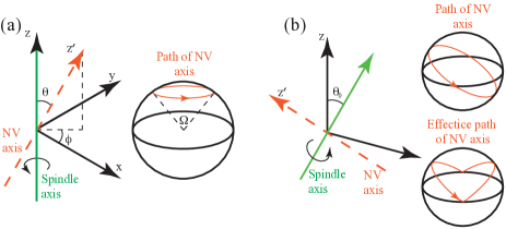
Figure 2: (a) Proposed Ramsey geometry. The crystal is attached to a rotating spindle with the NV ($z^{\prime}$) axis of one of its NV centers at an angle $\theta$ to the spindle ($z$) axis. Rabi pulses are produced by a microwave field linearly polarised with its magnetic field oscillating along the $z$-axis. The magnitude of the geometric phase after a complete rotation of the spindle is given by the solid angle subtended by the $z^{\prime}$-axis. (b) Proposed spin echo geometry. The spindle is at an angle $\theta_{0}$ to the fixed $z$ axis of the microwave field, and the NV axis is perpendicular to the spindle axis. The actual path of the NV ($z^{\prime}$) axis encloses a solid angle of $2\pi$, which is not observable. The $\pi$-pulse in the spin echo geometry, however, rectifies the alternating Berry phase accumulation, producing a total phase of $4\theta_{0}$ after a full spindle rotation, the solid angle enclosed by the effective trajectory shown.

The geometric phase, given initialisation into $\psi_{z^{\prime}}^{(m)}$, after the crystal has been rotated along a trajectory $P$, defined as rotation about the $z$-axis with fixed $\theta$, is given by

$$\Phi=\int_{0}^{t}\left[\frac{d\psi_{z^{\prime}}^{(m)}(t)}{dt}\right]^{\star}\psi_{z^{\prime}}^{(m)}(t)dt=\int_{P}m\left(1-\cos\theta\right)d\phi.$$ (18)

A similar effect occurs if the quantization axis is determined by an electric field, which is rotated Book . For a closed loop in parameter space, this is simply the solid angle enclosed by the trajectory of $z^{\prime}$, see Fig. 2(a). In the derivation of Eq. (18) we have assumed that the evolution of the system is adiabatic: $\dot{\theta}^{2}+\sin^{2}\theta\dot{\phi}^{2}\ll 2D^{2}$, i.e. the adiabatic approximation is valid provided the angular velocity of the crystal is much less that the zero-field splitting frequency, which is true for the cases we consider below.

While there is a gauge degree of freedom in defining the instantaneous eigenstates $\psi_{z^{\prime}}^{(m)}$, the geometric phase for a closed loop trajectory is independent of the choice of gauge. However, we are interested in a geometric phase for trajectories which are not closed loops and must then be careful in choosing our gauge.

The geometric phase is observed through interaction with a microwave magnetic field ${\bm{B}_{R}}$ and it is the phase difference between the NV center and the microwave field, as seen by the NV center, which is the observable quantity. Consider a linearly polarized microwave field tuned to the zero-field splitting transition, oscillating along the fixed $z$ axis, ${\bm{B}_{R}}=B_{R}\cos(\omega t)\hat{z}$. The Hamiltonian for the interaction of this field with the NV center is

$$H_{{\rm int}} = \frac{g\mu_{B}}{\hbar}{\bm{B}_{R}}\cdot{\bm{S}}$$ (22)

$$= g\mu_{B}B_{R}\cos(\omega t)\left(\begin{array}[]{ccc}\cos\theta&\frac{e^{i\phi}\sin\theta}{\sqrt{2}}&0\\ \frac{e^{-i\phi}\sin\theta}{\sqrt{2}}&0&\frac{e^{i\phi}\sin\theta}{\sqrt{2}}\\ 0&\frac{e^{-i\phi}\sin\theta}{\sqrt{2}}&-\cos\theta\end{array}\right)_{z^{\prime}}$$

$$\approx g\mu_{B}B_{R}\cos(\omega t)\frac{\sin\theta}{\sqrt{2}}\left(\begin{array}[]{ccc}0&e^{i\phi}&0\\ e^{-i\phi}&0&e^{i\phi}\\ 0&e^{-i\phi}&0\end{array}\right)_{z^{\prime}},$$ (26)

where the matrices are expressed with respect to the $|m\rangle_{z^{\prime}}$ basis as defined by Eq. (17). The approximation neglects the term proportional to $S_{z^{\prime}}$ and is valid for weak microwave fields: $g\mu_{B}B_{R}/\hbar\ll\omega$.

Equation (26) depends on both the polar $\theta$ and azimuthal $\phi$ angles. The dependence on the polar angle is simply a matter of effective strength, i.e. the effective microwave field strength experienced by the NV center is just $B_{R}\sin\theta$. The dependence on the azimuthal angle is more interesting: it has the character of a phase. The effect of a microwave pulse on state $\psi_{z^{\prime}}^{(m)}$ when the NV axis is at some azimuthal angle $\phi=\phi_{0}$ is the same as the effect when $\phi=0$ and the eigenstate is modified by a phase factor $\exp(-im_{z^{\prime}}\phi_{0})$. Since the linearly polarised microwave field can be decomposed into two counter-rotating fields, it should be no surprise that the effective phase of the NV center should be so closely linked to the microwave field’s angle relative the the NV axis.

This phase-like dependence of the interaction Hamiltonian on the NV orientation can be eliminated via a gauge transformation, of the $\psi_{z^{\prime}}^{(m)}$ basis, of the form

$$\psi_{z^{\prime}}^{(m)}\rightarrow e^{if_{m}(\theta,\phi)}\psi_{z^{\prime}}^{(m)}.$$ (27)

Choosing $f_{m}=-m\phi$ eliminates the $\phi$-dependence of the interaction Hamiltonian [Eq. (26)] as desired. This change of gauge does not alter measurable quantities. Using this gauge transformed eigenstate basis the geometric phase becomes

$$\Phi=\int_{P}m\cos\theta d\phi.$$ (28)

The final state produced by the microwave pulse now depends only on the explicit phase given by Eq. (28).

The challenge is now to measure the relative phase accumulation between two states. Because the bulk diamond NV electron spin has such long coherence times it should be possible to observe a geometric phase by mechanically spinning a diamond crystal. The set-up we propose is very similar to the Aharonov-Casher measurement proposed in Ref. Maclaurin09 . A diamond crystal is mounted on a spinning spindle. Optical initialisation, coherent microwave control, and fluorescence detection are used to measure the phase evolved after a certain rotation angle. Below we consider two possible scenarios for measuring the geometric phase: a relatively simple Ramsey geometry [Fig. 2(a)] and a spin echo pulse sequence [Fig. 2(b)], enabling a significant increase in the maximum geometric phase observed at the cost of introducing additional $\pi$ microwave pulses. In each case it is assumed that the microwave pulse durations and readout times are of order $50$ ns and hence the diamond can be considered to be stationary. Finally the relative sensitivity of the measurements is investigated.

The Ramsey geometry is shown in Fig. 2(a), with the microwave field linearly polarised with its magnetic field pointing along the spindle ($z$) axis. The crystal itself is mounted such that the NV axis makes an angle $\theta$ to the spindle axis. To remove the degeneracy of the $\psi_{z^{\prime}}^{(\pm 1)}$ states we assume a magnetic field rotating with the spindle, produced, for example, by a permanent magnet mounted on the spindle.

For the Ramsey geometry as the azimuthal angle $\phi$ of the NV axis passes zero, a $\pi/2$ Rabi pulse is applied, tuned to the $\psi_{z^{\prime}}^{(0)}\rightarrow\psi_{z^{\prime}}^{(1)}$ transition. As the spindle continues to rotate, a relative geometric phase evolves between the $\psi_{z^{\prime}}^{(0)}$ and $\psi_{z^{\prime}}^{(1)}$ states, given by $\Phi=\phi\cos\theta$. Since the magnetic field, used to split the $\psi_{z^{\prime}}^{(\pm 1)}$ states, is static the only phase accumulated between the states is $\Phi$. After the spindle has rotated through some angle $\phi_{0}$, a second $\pi/2$ pulse is applied, converting the phase into a population difference, which is measured by $532$ nm illumination and a fluorescence recording. A spindle rotation frequency of $\Omega=4000\pi$ rad/s and a $10$ $\mu$s inhomogeneous broadening time ($T^{*}_{2}$) Jelezko04 would allow up to $20$ mrad of geometric phase to be accumulated.

To extend the coherence lifetime of the NV electron spin a spin echo pulse sequence could be employed, hence enabling a larger geometric phase to be measured. To do this a different geometry is required, shown in Fig. 2(b), in which the spindle axis is placed at an angle $\theta_{0}$ to the microwave field ($z$) axis, and the NV ($z^{\prime}$) axis is perpendicular to the spindle axis. The resulting geometric phase, alternates, and for a complete rotation is zero.

A spin echo control sequence, with $\pi$ pulses applied whenever the NV ($z^{\prime}$) axis is perpendicular to $z$, would rectify the alternating geometric phase, producing a total phase of $\Phi=4n\theta$, where $n$ is the number of complete spindle rotations. By extending the coherence time from $T_{2}^{*}$ to $T_{2}\approx 2$ ms Balasubramanian09 a spin echo control sequence enables a geometric phase difference of $4$ radians to be produced.

The measurements proposed above would consist of many repetitions of the pulse sequence to get an average signal. The sensitivity of the measurement of the geometric phase is determined by the Poissonian statistics of spin projection, photon emission, and photon collection. The uncertainty $\Delta\Phi$ in the measurement of a geometric phase is related to the uncertainty $\Delta S$ of the normalised fluorescence signal $S$,

$$\Delta\Phi=\Delta S\left(\frac{dS}{d\Phi}\right)^{-1}=2\Delta S.$$ (29)

The second equality arises because the normalised signal, a sinusoidal function of $\Phi$, has a maximum gradient of $1/2$. By appropriately retarding the phase of the final $\pi/2$ pulse it can be ensured that the sinusoid is at its steepest point at the time of measurement.

The normalised signal $S$ is the number of photons collected over $N_{r}$ runs, normalised so that $\langle S\rangle=1/2$ when the populations of $\psi_{z^{\prime}}^{(0)}$ and $\psi_{z^{\prime}}^{(1)}$ are equal. If each measurement of $\psi_{z^{\prime}}^{(0)}$ or $\psi_{z^{\prime}}^{(1)}$ corresponded to the emission and detection of exactly one or zero photons respectively, then the variance of $S$ would be $(\Delta S)^{2}=1/(2N_{r})$. A more careful analysis, taking into account the statistics of (spontaneous) photon emission, imperfect detection and the nonzero fluorescence of the $\psi_{z^{\prime}}^{(1)}$ state, modifies the variance of the normalised signal by a factor $C^{2}$, giving $(\Delta S)^{2}=1/(2C^{2}N_{r})$. The physical basis for the factor $C$ ($C\approx 0.15$ for typical experiments and $C=1$ in the ideal case) is described by Taylor et al. Taylor08 .

The relative sensitivity for a series of geometric phase measurements, using a single NV center, is

$$\frac{\Delta\Phi}{\Phi}\approx\frac{2\pi\sqrt{2T_{M}}}{C\Omega T_{2}^{(*)}\sqrt{T_{T}}},$$ (30)

where $T_{M}$ is the time to take a single measurement, $T_{T}$ is the total averaging time. Expressing $T_{M}$ in terms of the relevant de-coherence time ($T_{M}=aT_{2}^{(*)}$, where $a>1$) the relative sensitivity becomes

$$\frac{\Delta\Phi}{\Phi}\sqrt{T_{T}}\approx\frac{2\pi\sqrt{2a}}{C\Omega\sqrt{T_{2}^{(*)}}}.$$ (31)

Based on the proposed experimental parameters given above ($a=2$), this corresponds to a relative uncertainty in the measurement of $\Phi$ with (without) spin echo pulses sequences of $0.15$ Hz^-1/2 ($2$ Hz^-1/2), or a $0.15$% ($2$%) uncertainty after three hours.

An alternative approach to measuring a geometric phase using an NV centre is to make use of an ancillary nuclear spin. Coherent control of nearby nuclear spins such as ¹³C or ¹⁴N has been demonstrated experimentally Dutt07 ; Jiang09 ; Jelezko04a . Hyperfine coupling between the electron and nuclear spin allows controlled-not (CNOT) operations to be performed, conditionally flipping one spin depending on the value of the other spin, which allows information to be exchanged between electron and nuclear spins. The adiabatically varying Hamiltonian in a nuclear spin geometric phase experiment could come from a number of sources. It is known that the ¹⁴N spin of an NV centre has a $5$ MHz zero-field nuclear quadrupole splitting along the NV axis, in complete analogy with the zero-field splitting of the NV electronic spin. The zero-field splitting of a ¹³C spin, however, will depend on its location. One approach would be to split the nuclear spin states using a magnet mounted on the spindle which rotates with the crystal. The splitting of nuclear spin states will in any case be on the order of MHz, so adiabaticity (with kHz spindle rotation speed) is still maintained. Due to their weaker interaction (by three orders of magnitude) with the environment, nuclear spins have longer coherence times than electronic spins, $T^{*}_{2}$ on the order of ms Dutt07 for ¹³C spin. A geometric phase experiment using nuclear spin would thus be both more sensitive and would allow a complete rotation of the spindle within the coherence time at the expense of a more complicated pulse sequence.

We have demonstrated that a geometric phase shift manifests between the internal magnetic states of a single nitrogen-vacancy defect, within a rotating diamond crystal. The measurement of such a geometric phase shift in a macroscopically rotating single atom-scale quantum object would provide a unique test of our fundamental understanding of quantum mechanics. As such we have demonstrated that the measurement of geometric phase shifts of $>$ 1 radian in such systems is possible. The analysis presented above is not only important in terms of demonstrating geometric phase shifts in macroscopically rotating quantum systems it also provides the basis for quantifying geometric phase shift effects in the use of nano-diamonds as high precision translational and rotational sensors Dougal_Thesis ; Mcquinness11 ; Dima ; Paola .

This research was supported by the Australian Research Council Centre of Excellence for Quantum Computation and Communication Technology (CE110001027). L.C.L.H. was supported under an Australian Research Council Professorial Fellowship (DP0770715).

References

- (1) Y. Aharonov and D. Bohm, Phys. Rev. 115, 485 (1959).
- (2) M.V. Berry, Proc. R. Soc. London A 392, 45 (1984).
- (3) Geometric Phases in Physics, edited by A. Shapere and F. Wilczek (World Scientific, Singapore, 1989).
- (4) J. Anandan, Nature 360, 307 (1992).
- (5) Y. Aharonov and A. Casher, Phys. Rev. Lett. 53, 319 (1984).
- (6) R.C. Casella, Phys. Rev. Lett. 65, 2217 (1990).
- (7) X.-G. He and B.H.J. McKellar, Phys. Rev. A 64, 022102 (2001).
- (8) S. Pancharatnam, Proc. Ind. Acad. Sci. 44, 247 (1956).
- (9) C.A. Mead and D.G. Truhlar, J. Chem. Phys. 70, 2284 (1979).
- (10) C.A. Mead, Chem. Phys. 49, 23 (1980).
- (11) R. Jackiw, Int. J. Mod. Phys. A 3 285 (1988).
- (12) C.A. Mead, Rev. Mod. Phys. 64, 51 (1992).
- (13) A. Shapere and F. Wilczek, J. Fluid Mech. 198, 557 (1989).
- (14) B. Simon, Phys. Rev. Lett. 51, 2167 (1983).
- (15) D. Arovas, J.R. Schrieffer and F. Wilczek, Phys. Rev. Lett. 53, 722 (1984).
- (16) M. Stone, Phys. Rev. D 33, 1191 (1986).
- (17) R. Tycko, Phys. Rev. Lett. 58, 2281 (1987).
- (18) S. Appelt, G. Wäckerle and M. Mehring, Phys. Rev. Lett. 72, 3921(1994).
- (19) N.B. Manson, J.P. Harrison and M.J. Sellars, Phys. Rev. B 74, 104303 (2006).
- (20) M. Steiner, P. Neumann, J. Beck, F. Jelezko and J. Wrachtrup, Phys. Rev. B 81, 035205 (2010).
- (21) D. Budker, D.F. Kimball and D.P. DeMille, Atomic Physics: An Exploration Through Problems and Solutions, Ed. (Oxford University Press, New York, 2008).
- (22) D. Maclaurin, A.D. Greentree, J.H. Cole, L.C.L. Hollenberg and A.M. Martin, Phys. Rev. A 80, 040104(R) (2009).
- (23) F. Jelezko, T. Gaebel, I. Popa, A. Gruber and J. Wrachtrup, Phys. Rev. Lett. 92, 076401 (2004).
- (24) G. Balasubramanian et al., Nature Materials 383 (2009).
- (25) J.M. Taylor et al., Nature Physics 4, 810 (2008).
- (26) M.V.G. Dutt et al., Science 316, 1312 (2007).
- (27) L. Jiang et al., Science 326, 267 (2009).
- (28) F. Jelezko et al., Phys. Rev. Lett. 93, 130501 (2004).
- (29) D. Maclaurin, From Geometric Phases to Intracellular Sensing: New Applications of the Daimond Nitrogen-Vacancy Centre (MPhil Thesis, University of Melbourne, 2010).
- (30) L.P. Mcguinness, et al., Nature Nanotechnology 6, 358 (2011).
- (31) M. Ledbetter, K. Jensen, R. Fischer, A. Jarmola and D. Budker, arXiv:1205.0093.
- (32) A. Ajoy and P. Cappellaro, arXiv:1205.1494