Local kernel canonical correlation analysis with application to virtual drug screening

Abstract

Drug discovery is the process of identifying compounds which have potentially meaningful biological activity. A major challenge that arises is that the number of compounds to search over can be quite large, sometimes numbering in the millions, making experimental testing intractable. For this reason computational methods are employed to filter out those compounds which do not exhibit strong biological activity. This filtering step, also called virtual screening reduces the search space, allowing for the remaining compounds to be experimentally tested.

In this paper we propose several novel approaches to the problem of virtual screening based on Canonical Correlation Analysis (CCA) and on a kernel-based extension. Spectral learning ideas motivate our proposed new method called Indefinite Kernel CCA (IKCCA). We show the strong performance of this approach both for a toy problem as well as using real world data with dramatic improvements in predictive accuracy of virtual screening over an existing methodology.

copyrightownerIn the Public Domain

, , , and t1Supported in part by NSF Grant DMS-07-47575 and NIH Grant NIH/NCI R01 CA-149569. t2Supported in part by NIH Grant GM066940.

1 Introduction

Computer-Aided Drug Discovery (CADD) is an area of research that is concerned with the identification of chemical compounds that are likely to possess specific biological activity, that is, the ability to bind certain target biomolecules such as proteins. CADD approaches are employed in order to prioritize molecules in commercially available chemical libraries for experimental biological screening. The prioritization of molecules is critical since these libraries frequently contain many millions of molecules making experimental testing intractable. The process of using computational methods to filter out those compounds which are not expected to exhibit strong biological activity is called virtual screening.

Computational methods have been used extensively to assist in experimental drug discovery studies. In general, there are two major computational drug discovery approaches, ligand based and structure based. The former is used when the three-dimensional structure of the drug target is unknown but the information about a reasonably large number of organic molecules active against a specific set of targets is available. In this case, the available data can be studied using cheminfomatic approaches such as Quantitative Structure-Activity Relationship (QSAR) modeling [for a review of QSAR methods see A. Tropsha, in Abraham (2003)]. In contrast, the structure-based methods rely on the knowledge of three-dimensional structure of the target protein, especially its active site; this data can be obtained from experimental structure elucidation methods such as X-ray or Nuclear Magnetic Resonance (NMR) or from modeling of protein three-dimensional structure.

Virtual screening is one of the most popular structure-based CADD approaches where, typically, three-dimensional protein structures are used to discover small molecules that fit into the active site (a process referred to as docking) and have high predicted binding affinity (scoring). Traditional docking protocols and scoring functions rely on explicitly defined three-dimensional coordinates and standard definitions of atom types of both receptors and ligands. Albeit reasonably accurate in some cases, structure-based virtual screening approaches are for the most part computationally inefficient [Warren et al. (2006)]. As a result of computational inefficiency there is a limit to the number of compounds which can reasonably be screened by these methods. Furthermore, recent extensive studies into the comparative accuracy of multiple available scoring functions suggest that accurate prediction of binding orientations and affinities of receptor–ligand pairs remains a formidable challenge [Kitchen et al. (2004)]. Yet millions of compounds in available chemical databases and billions of compounds in synthetically feasible chemical libraries are available for virtual screening calling for the development of approaches that are both fast and accurate in their ability to identify a small number of viable and experimentally testable computational hits.

Recently, we introduced a novel structure-based cheminformatic workflow to search for Complimentary Ligands Based on Receptor Information (CoLiBRI) [Oloff et al. (2006)]. This novel computational drug discovery strategy combines the strengths of both structure-based and ligand-based approaches while attempting to surpass their individual shortcomings. In this approach, we extract the structure of the binding pocket from the protein and then represent both the receptor active site and its corresponding ligand in the same universal, multidimensional chemical descriptor space (note that in principle, the descriptors used for receptors and ligands do not have to be the same, and we will be exploring the use of different descriptor types in future studies). We reasoned that mapping of both binding pockets and corresponding ligands onto the same multidimensional chemistry space would preserve the complementary relationships between binding sites and their respective ligands. Thus, we expect that ligands binding to similar active sites are also similar. In cheminformatics applications, the similarity is described quantitatively using one of the conventional metrics, such as Manhattan or Euclidean distance in multidimensional descriptor space. Thus, the chief hypothesis in CoLiBRI is that the relative location of a novel binding site with respect to other binding sites in multidimensional chemistry space could be used to predict the location of the ligand(s) complementary to this site in the ligand chemistry space. After generation of descriptors, the dataset is split into training and test sets and then variable selection is carried out to generate models optimizing this complementarity between the binding pocket and ligand spaces. These models are then applied to a binding pocket in a protein of interest to generate a predicted virtual ligand point which is used as a query in chemical similarity searches to identify putative ligands of the receptor in available chemical databases. In this paper, we build upon the work of Oloff et al. (2006) to develop a substantially more advanced and efficient version of CoLiBRI.

The problem can be generally stated as follows: for a set of $n$ known protein–ligand pairs, with $d_{X}$ and $d_{Y}$ descriptors, respectively, given a new protein we want to be able to predict what ligand(s) will bind to it. Two virtual drug screens will be used as a benchmark for testing the methods discussed and developed here: [(2)]

A set of 800 chemically and functionally diverse protein–ligand pairs obtained from the Protein Data Bank (PDB) database on experimentally measured binding affinity (PDBbind) [Wang et al. (2004)]. These compounds are described by a set of 150 chemical descriptors. These descriptors include information related to the electronic attributes, hydrophobicity and steric properties of the compounds. For a more detailed discussion on the different types of chemical descriptors, see Todeschini and Consonni (2009a, 2009b). We will refer to this data set as the 800 Receptor–Ligand pairs (RLP800) data. Results and further details on this and two additional data sets can be found in Section 1.1.

The World Drug Index (WDI) [Daylight (2004)] database which contains approximately 54,000 drug candidates (ligands). Each compound in the WDI is described by the same set of 150 chemical descriptors as the RLP800 data.

The accuracy of our prediction is based on how close, in Euclidean distance, our prediction is to the actual ligand. This is then compared against the distances of all of the ligands in the space to the actual ligand. A standard measure of predictive accuracy used in the QSAR literature [Tropsha (2003), Oloff et al. (2006)] is based on ranking these distances, from smallest to largest. Defining $r_{i}$ to be the rank of our prediction of test ligand $i$, model performance is defined as the average rank over each of the new points we are trying to predict, $\bar{r}=\sum_{i=1}^{n_{T}}r_{i}$. This criterion reflects the average size of the search space needed to find each compound. Here $n_{T}$ denotes the number of new (i.e., test) ligands we are predicting.

The $\bar{r}$ effectiveness of the methods studied and developed here is illustrated in Figure 1. Figure 1(A) is a histogram of the ranks, $r_{i}$ for our novel method which is a variant of Canonical Correlation Analysis (CCA) we call Indefinite Kernel CCA (IKCCA) (Section 4), on the RLP800 data.

The previous state of the art for these data sets is $\bar{r}_{\mathrm{OLOFF}}$ (the vertical line furthest to the right labelled Oloff et al.) which are larger by a factor of 5 to 10 as compared to CCA (Section 2) and its improvements, KCCA (Section 3) and IKCCA.

As we were primarily interested in comparing our results against those of Oloff et al. (2006) we did not look into other performance metrics other than mean rank. However, it would be interesting to pursue other, potentially more relevant measures of binding affinity such as Kd, Ki and IC50 as was done by Witten and Tibshirani (2009), where CCA is linked to these performance measures.

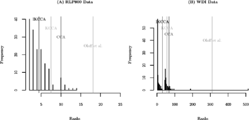
Figure 1: (A) A histogram showing the IKCCA ranks, $r_{i}$, resulting from prediction on the test data from the RLP800 dataset. (B) Performance on the WDI data.

While not discussed in this paper, an important unresolved issue in this cheminformatic-based approach to the prediction of protein–ligand binding is the selection of meaningful chemical descriptors. The type of chemical descriptors used can have a drastic effect on the predictive accuracy of an algorithm. One possible approach to addressing this issue would be to use a recently developed method called Sparse CCA (SCCA), Hardoon and Shawe-Taylor (2008), Parkhomenko (2008), Witten, Tibshirani and Hastie (2009) and Witten and Tibshirani (2009). SCCA uses a lasso-like approach to identify sparse linear combinations of two sets of variables that are highly correlated with each other. An approach based on SCCA to the prediction of protein–ligand binding may prove to be quite useful in resolving some of the issues arising from chemical descriptor selection.

In Section 1.1 we present results and details on the RLP800 data set as well as on two additional data sets. In Sections 2 and 3 we outline CCA and KCCA, respectively. In Section 4 we propose a new method, IKCCA, which encompasses nonpositive semi-definite (PSD) kernels (i.e., indefinite kernels), specifically we consider a class of kernels related to the Normalized Graph Laplacian used in Spectral Clustering. Finally, in Section 5 we show how prediction of a new ligand is done using CCA (and its variants).

1.1 Additional drug discovery results

In addition to the real data results discussed in Section 1, we also tested our method on two additional data sets [which we refer to as Experimental Settings (ES), the reason for which will become clearer in what follows]. These data (including the RLP800 data) are subsets of a collection of 1,300 complexes taken from PDBBind [Wang et al. (2004)]. These 1,300 complexes are referred to as the Refined Set (RS), a set of entries that meet a defined set of criteria regarding crystal structure quality. A representative subsample of 195 of the complexes is called the Core Set (CS). This is a collection of complexes selected by clustering the RS into 65 groups using protein sequence similarity and retaining only 3 complexes from each cluster.

The three experimental settings considered are denoted by ES I [this experimental setting was used in Oloff et al. (2006)], ES II and ES III. In each of these experimental settings the RS and CS complexes are separated into training and testing sets in such a way as to test different aspects of our model. In ES I the 637 training and 163 test complexes are randomly sampled from the RS. ES I is meant to provide a general test of our models performance. In ES II the training (153 complexes) and testing (36 complexes) sets are sampled from the CS in such a way that the various protein families in the CS are well represented in both. This separation is meant to test the performance of our CCA-based methods when the sample size is small. Finally, in ES III the testing set (162 complexes) is composed of proteins which are under represented in the training set (1,006 complexes). This is meant to test our methods ability to correctly identify novel complexes.

Table 1: This table summarizes the performance of the method discussed in Oloff et al. (2006) as well as the methods developed in this paper on the CoLiBRI, Name and Cluster data sets. The columns labeled “Train” and “Test” correspond to the number of training and testing samples for a given data set. The column labeled “Embed” corresponds to the total number of ligands against which our prediction is to be ranked. The remaining columns correspond to the method used and the average rank performance of that method. Note that as the method used in Oloff et al. (2006) failed to provide useful results for the Name and Cluster data sets, no results were reported. In all cases IKCCA, using the NGL kernel, outperformed the other methods. In all cases the CCA-based methods provide considerable improvement over the previous approach

Setting		Train	Test	Embed	Oloff	CCA	KCCA	IKCCA
ES I	RS	1,637	$163$	54,800	$18.1$	$10$	$7.5$	$4.5$
	RS${}+{}$WDI			54,121	$310$	$67$	$56$	$30$
ES II	RS	1,153	$36$	54,189	NA	$8$	$13.75$	$3.5$
	RS${}+{}$WDI			53,994	NA	$275.1$	1,558	$92.9$
ES III	RS	1,006	$162$	51,168	NA	$11.9$	$7.4$	$4.4$
	RS${}+{}$WDI			54,120	NA	$53$	$24.3$	$18.2$

A note on how we use the training and testing sets: the tuning parameters for our model are selected, as discussed in Section 5.2, using only the training set. Once tuning parameters have been selected, prediction on the testing set is then performed. This is meant to test the models performance on as-yet unobserved complexes.

The results for each of these experimental settings is summarized in Table 1.1. The columns labeled “Train” and “Test” correspond to the size of the training/testing sets for each particular experimental setting. The column labeled “Embed” corresponds to the total number of ligands against which our prediction is to be ranked. The remaining columns correspond to the method used and the average rank performance (defined in Section 1) of that method. The second row, second column in each cell labeled “RS${}+{}$WDI” shows the results for each method on the Reduced Set plus the World Drug Index. These results are meant to more accurately mimic an actual drug screen by having a larger test set to search against. As the method used in Oloff et al. (2006) failed to provide useful results for the ES II and ES III experimental settings, no results are reported here. Generally speaking, in all cases IKCCA, using the NGL kernel, outperformed the other methods. All the CCA-based methods provide considerable improvement over the previous approach.

Looking a bit closer at the results it is interesting to note that while all three CCA-based methods performed worse on the ES II data, KCCA had the largest drop in performance. This can be seen by comparing the average rank performance against the total number of ligands we are searching against. The decrease in performance in all cases more than likely has to do with the small size of the training set. In the case of KCCA, its considerable decrease in performance, we suspect, may have to do with not having a large enough training sample to reliably select the bandwidth parameter $\sigma$. For IKCCA the adaptive nature of the local kernel is probably what allows it to perform well in the low sample size setting.

2 Canonical correlation analysis

CCA [Hotelling (1936)] naturally lends itself to the problem of predicting the binding between proteins and ligands. This can be understood for the following reasons: first, traditional methods of prediction, for example, regression, assume a direction of dependence between the variables to be predicted and the predictive variables. Here we have a symmetric, not causal, type of relationship: the binding between a protein and its ligand is inherently co-dependent. Second, in addition to capturing the dependence structure we are looking to model, CCA is well suited to the type of prediction we are interested in performing. To understand this, consider the following (see also Section 2.2.1 for a more detailed discussion). The objective of CCA is to find directions in one space, and directions in a second space such that the correlation between the projections of these spaces onto their respective directions is maximized. These directions are commonly referred to as canonical vectors. Let us assume that a set of directions are found so that the corresponding projections of proteins and of ligands are strongly correlated. Predicting a new ligand given a new protein would begin with projecting the new protein into canonical correlation space. Then, assuming the same correlation structure holds for this new point, prediction of the new ligand would amount to interpolating its location in ligand space based on the location of the protein in protein space. This will be discussed in greater detail in Section 5. Next we provide a brief discussion on the details of CCA and KCCA.

2.1 Canonical correlations

Let $\mathbf{x}_{i}\in\mathbb{R}^{d_{X}}$ and $\mathbf{y}_{i}\in\mathbb{R}^{d_{Y}}$, $i=1,\ldots,n,$ denote a protein–ligand pair. The sample of pairs is collected in matrices $\mathbf{X}\in\mathbb{R}^{n\times d_{X}}$ and $\mathbf{Y}\in\mathbb{R}^{n\times d_{Y}}$ with $\mathbf{x}_{i}$ and $\mathbf{y}_{i}$ as the descriptors for a row.

The objective of CCA is to find the linear combinations of the columns of $\mathbf{X}$ (proteins), say $\mathbf{X}\mathbf{w}_{X}$ and the linear combinations of the columns of $\mathbf{Y}$ (ligands), say $\mathbf{Y}\mathbf{w}_{Y}$ such that the correlation, $\operatorname{corr}(\mathbf{X}\mathbf{w}_{X},\mathbf{Y}\mathbf{w}_{Y})$ is maximized. Without loss of generality assume that the matrices $\mathbf{X}$ and $\mathbf{Y}$ have been mean centered. Letting $\mathbf{S}_{XX}=\mathbf{X}^{T}\mathbf{X}$, $\mathbf{S}_{YY}=\mathbf{Y}^{T}\mathbf{Y}$ and $\mathbf{S}_{XY}=\mathbf{X}^{T}\mathbf{Y}$ the CCA optimization problem is

$$\rho=\max_{\mathbf{w}_{X},\mathbf{w}_{Y}}\operatorname{corr}(\mathbf{X}\mathbf{w}_{X},\mathbf{Y}\mathbf{w}_{Y})$$

subject to, (1)

$$\mathbf{w}_{X}^{T}\mathbf{S}_{XX}\mathbf{w}_{X}=\mathbf{w}_{Y}^{T}\mathbf{S}_{YY}\mathbf{w}_{Y}=1.$$

Subsequent directions are found by imposing the additional constraints$(\mathbf{w}_{X}^{i})^{T}\times\mathbf{S}_{XX}\mathbf{w}_{X}^{j}=(\mathbf{w}_{Y}^{i})^{T}\mathbf{S}_{YY}\mathbf{w}_{Y}^{j}=(\mathbf{w}_{X}^{i})^{T}\mathbf{S}_{XY}\mathbf{w}_{Y}^{j}=0$ for $i\neq j$ and$(\mathbf{w}_{X}^{i})^{T}\mathbf{S}_{XX}\mathbf{w}_{X}^{i}=(\mathbf{w}_{Y}^{i})^{T}\mathbf{S}_{YY}\mathbf{w}_{Y}^{i}=1$, $i,j=1,\ldots,p$, $p=\operatorname{min}(d_{X},d_{Y})$.

In order to avoid issues arising from multicollinearity and singularity of the covariance matrices we impose a penalty [Vinod (1976)] on the directions $\mathbf{w}_{X}$ and $\mathbf{w}_{Y}$ so that the constraints in (2.1) are modified to be

$$\mathbf{w}_{X}^{T}\mathbf{S}_{XX}\mathbf{w}_{X}+\kappa\mathbf{w}_{X}^{T}\mathbf{w}_{X}=\mathbf{w}_{Y}^{T}\mathbf{S}_{YY}\mathbf{w}_{Y}+\kappa\mathbf{w}_{Y}^{T}\mathbf{w}_{Y}=1,$$ (2)

where $\kappa\in\mathbb{R}$ is a regularization parameter.

The predictive accuracy of this approach was discussed in Section 1, with results summarized in Figure 1. Recall that the lines in these figures labeled CCA correspond to the average predicted rank using CCA, which improved upon Oloff et al. (2006) shown by the lines labeled a such.

2.1.1 The geometry of CCA

An appealing aspect of CCA is its intuitive geometric interpretation [Anderson (2003) and Kuss and Graepel (2002)]. A geometric perspective lends itself to a better understanding of the general behavior of CCA, and provides further evidence of its applicability to the protein–ligand matching problem.

Taking a closer look at the $i$th canonical correlation, $\rho_{i}$, $i=1,\ldots,p$ ($p=\operatorname{min}(d_{X},d_{Y})$), in the optimization problem shown in (2.1), it can be seen that this quantity is in fact equal to the cosine of the angle between $\mathbf{a}_{X}^{i}=\mathbf{X}\mathbf{w}^{i}_{X}$ and $\mathbf{a}_{Y}^{i}=\mathbf{Y}\mathbf{w}^{i}_{Y}$ ($\mathbf{a}_{X}^{i}$ and $\mathbf{a}_{Y}^{i}$ are commonly referred to as canonical variates). With this in mind maximizing the cosine (i.e., correlation) can equivalently be thought of as minimizing the angle between $\mathbf{a}_{X}^{i}$ and $\mathbf{a}_{Y}^{i}$. Furthermore, it can be shown that minimizing the angle is equivalent to minimizing the distance between pairs of canonical variates,

$$\min_{\mathbf{w}^{i}_{X},\mathbf{w}^{i}_{Y}}\|\mathbf{X}\mathbf{w}^{i}_{X}-\mathbf{Y}\mathbf{w}^{i}_{Y}\|^{2}$$

subject to the constraints described in (2.1). Note that viewed in this way, in canonical correlation space, this amounts to finding a system of coordinates such that the distance between coordinates is minimized. This is a sense in which CCA is an appropriate approach to the protein–ligand matching problem.

As will be seen in Sections 3 and 4, this geometric interpretation of CCA extends naturally to KCCA and IKCCA. Note that the regularized variant of CCA does not have the same geometric interpretation, nonetheless viewing regularized CCA in this manner still provides useful insight into its behavior.

2.2 Toy examples

2.2.1 Toy example 1: Motivating CCA

Consider the protein–ligandmatching problem as outlined above. For this toy example we set $n=10$ and $d=2$. Suppose the descriptors for this toy example are Molecular Weight (MW) and Surface Area (SA) of the molecule. Recall that each row of $\mathbf{X}_{(10\times 2)}$ and each row of $\mathbf{Y}_{(10\times 2)}$ corresponds to an observation, a protein or a ligand, respectively, and the columns correspond to the descriptors MW and SA. The pairs are identified by a unique label, corresponding to IDs from the Protein Data Bank (PDB) (www.pdb.org). Figure 2 shows the two toy data sets.

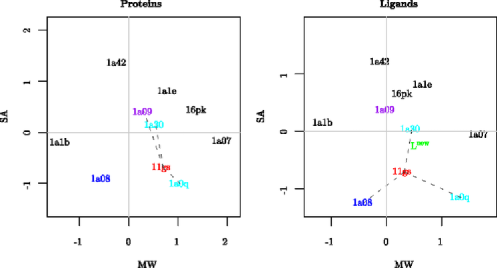
Figure 2: Toy example data. The points highlighted in red correspond to the protein–ligand pair 11gs, and the points connected to it by dashed black lines are its three nearest neighbors in each space. The observations highlighted in cyan are neighbors in both spaces, and those highlighted in blue and purple are neighbors only in the protein, and ligand spaces, respectively. The green point ${L}^{\mathrm{new}}$ in the ligand space corresponds to a weighted average (discussed in Section 5) of the cyan points and the purple point, that is, of the nearest neighbors of 11gs in the protein space.

From Figure 2 it can be seen that the distribution of points in the two spaces are quite similar in the sense that the location of corresponding points in the two spaces are close. The points connected to 11gs (red) by dashed black lines are its three nearest neighbors. The cyan points are neighbors shared in both spaces and the blue and purple points are mismatched. Two of three neighbors are shared in common (in the Euclidean sense).

Consider the case where the red point in ligand space is not observed and the task is to predict its value. Using the weighted average (see Section 5 for details on the derivation of the weights) of the points in ligand space that correspond to the nearest neighbors of the point 11gs in the protein space (points highlighted in cyan and purple in ligand space) would yield a relatively poor prediction despite the strong apparent similarity between the two distributions of points.

Next suppose that instead of carrying out the prediction of a new ligand in the original data space we carry out our prediction in canonical correlation space. Solving for $\mathbf{w}_{X}$ and $\mathbf{w}_{Y}$ in (2.1), gives us the canonical vectors shown in Figure 3. What is important to notice is how the distribution of points along the first and second canonical directions in both protein and ligand space are quite similar. This is due to the property of alignment that arises naturally from maximizing the correlation.

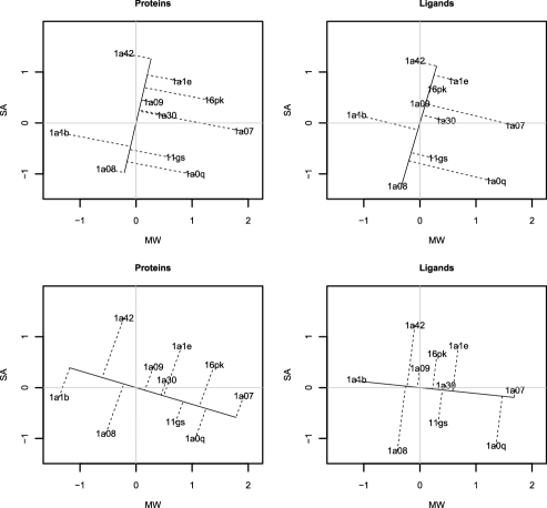
Figure 3: The direction vectors and the projected value of each point. The top row of plots shows the first direction vector and the projections onto it. The bottom row of plots show the second direction vector and the projection onto it.

Figure 4 shows the projections of the data onto the first two canonical vectors (note that separate directions are found in protein and ligand space). We can see that with the slight modification in alignment that has resulted from the CCA projections, the point 11gs now shares the same neighbors in both spaces. In particular note that now the predicted value in the projected ligand space is closer to the actual value (again using the weighted average).

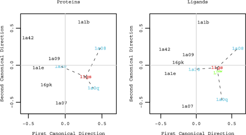
Figure 4: Projection of the data in Figure 2 onto the first and second canonical vectors. In contrast to Figure 2, the point 11gs now shares the same neighbors in both spaces and the predicted value in green is much closer to the actual value.

This example was deliberately chosen to illustrate the case where CCA is effective. However, in most cases the relationship between points in different spaces may be far more complicated, as we now illustrate.

2.2.2 Toy example 2: CCA challenge

We now consider an example where the relationship between spaces is more complex. Suppose that we have the same general framework as in Section 2.2.1 but rather than having both protein and ligand space characterized by MW and SA, we now have that the space of proteins has descriptors $d_{X}^{1}$ and $d_{X}^{2}$ and that the space of ligands has descriptors $d_{Y}^{1}$ and $d_{Y}^{2}$, shown in Figure 5. As before the observation highlighted in red, 1a94, corresponds to a new protein whose corresponding ligand we are trying to predict. The point highlighted in cyan is one of the 3-nearest neighbors of 1a94 in both spaces. Those points highlighted in purple (and blue) are nearest neighbors in only the protein (and ligand) spaces, respectively. The point $L^{\mathrm{new}}$ in the ligand space, highlighted in green is a weighted average of the nearest neighbors of the point 1a94 in protein space. Using $L^{\mathrm{new}}$ as a prediction of the new ligand would not provide a particularly accurate prediction.

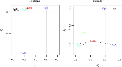
Figure 5: A plot of the data generated such that the underlying relationship between points is nonlinear. The observation highlighted in red, 1a94, is the new observation which we are trying to predict. The points joined to it by dashed black lines are its nearest neighbors. The points highlighted in cyan correspond to points that are nearest neighbors of 1a94 in both spaces. Points highlighted in purple and blue correspond to points that are only neighbors in either protein or ligand space, respectively. The point labeled $L^{\mathrm{new}}$ in ligand space corresponds to a weighted average of the points 1a08, 1a09 and 1a1b, that is, the nearest neighbors of the point 1a94 in protein space.

As before, we use CCA to try and find a linear combination of the descriptors which best align the two spaces. Figure 6 is a plot of the projections onto the first and second canonical variates in protein and ligand space. The color scheme is the same as in Figure 5. As can be seen, standard CCA does not seem to be able to find a good alignment between the two spaces, which is confirmed by the relatively low values of the canonical correlations, 0.79 and 0.54, respectively, for the first and second directions.

In Section 3 we show how mappings into a kernel induced feature space can be used to improve prediction. This will lead to our discussion of KCCA.

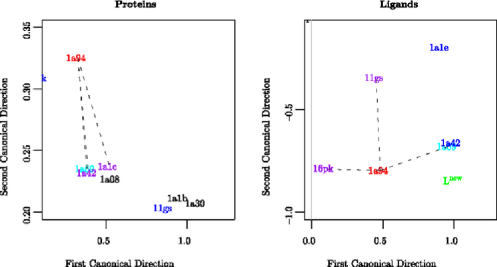
Figure 6: A plot of the data projected onto the first two canonical vectors in both protein and ligand spaces. The directions found by standard CCA do not provide a good alignment between the two spaces.

3 Kernel canonical correlation

3.1 Toy example 2: CCA challenge (motivating KCCA)

Returning to the example in Section 2.2.2, suppose it is believed that some type of functional relationship exists between the descriptors across spaces that is best characterized by looking at the second order polynomials of the descriptors within each space, that is,

$$\Phi_{X}\dvtx(d_{X}^{1},d_{X}^{2}) \rightarrow ((d_{X}^{1})^{2},(d_{X}^{2})^{2},d_{X}^{1}d_{X}^{2}),$$

$$\Phi_{Y}\dvtx(d_{Y}^{1},d_{Y}^{2}) \rightarrow ((d_{Y}^{1})^{2},(d_{Y}^{2})^{2},d_{Y}^{1}d_{Y}^{2}).$$

Figure 7 shows plots of proteins and ligands embedded into this three dimensional space. As can be seen there are now two neighbors shared in common between spaces (colored in cyan). Furthermore the prediction of the new observation, $L^{\mathrm{new}}$ (in green) by a weighted average of its three nearest neighbors in feature space is, by comparison, much closer to the actual value than the corresponding prediction in object space.

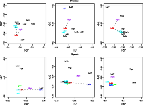
Figure 7: A plot of protein and ligand data in feature space. The color scheme is the same as in Figure 5. Looking at the plots on the top and bottom (corresponding to protein and ligand space, respectively), the overall correspondence between points in protein space and ligand space is much better than in the original (object) space. This improved mapping will allow CCA to do a better job aligning the two spaces.

As before CCA is used on this transformed data, now in feature space, to align the space of proteins and ligands. Figure 8 shows a plot of the projected data. Note that now both the new protein and its ligand (highlighted in red) share three neighbors and that the distribution of points within each of the spaces is quite similar. The quality of the alignment is further confirmed by looking at the canonical correlation values which are near 1 for each of the first two directions. Since the value of the third canonical correlation is considerably smaller (approximately 0.2) we only project onto the first two directions.

It is worth noting that, as a result of overfitting, the kernel canonical correlation values can sometimes be artificially large due to strong correlation between features in kernel space. Regularization methods for helping to control these effects in the kernel case will be discussed in Section 3.2.

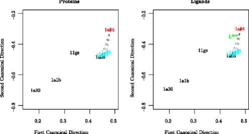
Figure 8: This is a plot of the projection of the data in protein and ligand feature space onto the first and second canonical vectors (note that we do not project onto the third canonical vector as the corresponding canonical correlation is relatively small, approximately 0.2). As can be seen, not only does the new observation 1a94 (red) have three neighbors in common in both protein and ligand space but the prediction of the new ligand using a weighted average, $L^{\mathrm{new}}$ highlighted in green on the plot on the right is close to the actual value of 1a94.

In general, finding explicit mappings such as those in (3.1) is impractical or simply not possible as in some cases this would require an infinite dimensional feature space. As we will see in the following section, kernels allow us to avoid such issues.

3.2 Kernel canonical correlation analysis

KCCA [Bach and Jordan(2002), Lai and Fyfe (2000), Hardoon, Szedmak and Shawe-Taylor (2004)] extends CCA by finding directions of maximum correlation in a kernel induced feature space. Let $\phi_{X}$ and $\phi_{Y}$ be the feature space maps for proteins and ligands, respectively. The sample of pairs, now mapped into feature space, are collected in matrices $\Phi_{X}$ and $\Phi_{Y}$ with $\phi_{X}(\mathbf{x}_{i})$ and $\phi_{Y}(\mathbf{y}_{i})$ as their respective row elements. The objective, as before, is to find linear combinations, $\Phi_{X}\mathbf{w}_{X}$ and $\Phi_{Y}\mathbf{w}_{Y}$ such that the correlation, $\operatorname{corr}(\Phi_{X}\mathbf{w}_{X}$, $\Phi_{Y}\mathbf{w}_{Y})$, is maximized. Note that because $\mathbf{w}_{X}$ and $\mathbf{w}_{Y}$ lie in the span of $\Phi_{X}$ and $\Phi_{Y}$, these can be re-expressed by the linear transformations $\mathbf{w}_{X}=\Phi_{X}\alpha_{X}$ and $\mathbf{w}_{Y}=\Phi_{Y}\alpha_{Y}$. Letting $\mathbf{K}_{X}=\Phi_{X}\Phi_{X}^{T}$ and $\mathbf{K}_{Y}=\Phi_{Y}\Phi_{Y}^{T}$ with $k_{X}$ and $k_{Y}$ being the associated kernel functions for each space, respectively, the CCA optimization problem in (2.1) now becomes

$$\hskip 35.0pt\rho_{\mathcal{H}}=\max_{\mathbf{w}_{X},\mathbf{w}_{Y}}\operatorname{corr}(\Phi_{X}\mathbf{w}_{X},\Phi_{Y}\mathbf{w}_{Y})=\max_{\alpha_{X},\alpha_{Y}}\operatorname{corr}(\mathbf{K}_{X}\alpha_{X},\mathbf{K}_{Y}\alpha_{Y})$$

subject to (4)

$$\hskip 35.0pt\mathbf{w}_{X}^{T}\Phi_{X}^{T}\Phi_{X}\mathbf{w}_{X}=\alpha_{X}^{T}\mathbf{K}_{X}^{2}\alpha_{X}=1\ \ \mbox{and}\ \ \mathbf{w}_{Y}^{T}\Phi_{Y}^{T}\Phi_{Y}\mathbf{w}_{Y}=\alpha_{Y}^{T}\mathbf{K}_{Y}^{2}\alpha_{Y}=1.$$

Here the subscript $\mathcal{H}$ in $\rho_{\mathcal{H}}$ is included to emphasize the fact that the space of functions we are considering are in a RKHS. Subsequent directions are found by including the additional constraints that $\alpha_{X}^{iT}\mathbf{K}_{X}^{2}\alpha_{X}^{j}=\alpha_{Y}^{iT}\mathbf{K}_{Y}^{2}\alpha_{Y}^{j}=\alpha_{X}^{iT}\mathbf{K}_{X}\mathbf{K}_{Y}\alpha_{Y}^{j}=0$ for $i\neq j$, and $\alpha_{X}^{iT}\mathbf{K}_{X}^{2}\alpha_{X}^{i}=\alpha_{Y}^{iT}\mathbf{K}_{Y}^{2}\alpha_{Y}^{i}=1$, $i,j=1,\ldots,n$.

In order to avoid trivial solutions, we penalize the directions $\alpha_{X}$ and $\alpha_{Y}$ modifying the constraints in (3.2) to be

$$\alpha_{X}^{T}\mathbf{K}_{X}^{2}\alpha_{X}+\kappa\alpha_{X}^{T}\alpha_{X}=\alpha_{Y}^{T}\mathbf{K}_{Y}^{2}\alpha_{Y}+\kappa\alpha_{Y}^{T}\alpha_{Y}=1.$$ (5)

Here $\kappa$ is a regularization parameter.

Note that the geometric interpretation of (unregularized) KCCA, provided that data have been centered in feature space, is the same as CCA. The only difference lies in the fact that the space in which this geometry is observed is in feature space rather than object space.

In order for KCCA to be understood as maximizing correlation in feature space centering must be performed in feature space. Centering in feature space can be done as follows. Let $\bar{\Phi}=\frac{1}{n}\mathbf{J}\Phi$ where $\mathbf{J}$ is an $n\times n$ matrix of ones, then

$$(\Phi-\bar{\Phi})(\Phi-\bar{\Phi})^{T} = \Phi\Phi^{T}-\Phi\bar{\Phi}^{T}-\bar{\Phi}\Phi^{T}+\bar{\Phi}\bar{\Phi}^{T}$$

$$= \mathbf{K}-\frac{1}{n}\mathbf{J}\mathbf{K}-\frac{1}{n}\mathbf{K}\mathbf{J}+\frac{1}{n^{2}}\mathbf{J}\mathbf{K}\mathbf{J}$$

$$= \biggl{(}\mathbf{I}-\frac{1}{n}\mathbf{J}\biggr{)}\mathbf{K}\biggl{(}\mathbf{I}-\frac{1}{n}\mathbf{J}\biggr{)}.$$

We assume throughout that the kernel matrices are centered.

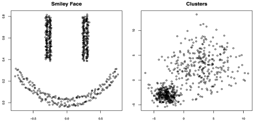
Figure 9: A toy example illustrating the cases when the distribution of points within a space is nonstandard and heterogeneous.

The predictive accuracy of this approach was discussed in Section 1, with results summarized in Figure 1. Recall that the cyan line in Figure 1 corresponds to the average predicted rank using KCCA which is an improvement over both Oloff et al. (2006) and CCA.

3.3 Toy example 3: KCCA challenge

We saw in Section 3.1 that KCCA was able to overcome some of the obstacles encountered by standard CCA. Where KCCA begins to encounter problems is when the distribution of points within a space is nonstandard and/or heterogeneous. To illustrate this consider the example shown in Figure 9, as with the protein–ligand matching problem, there is a one-to-one correspondence between points in the two spaces.

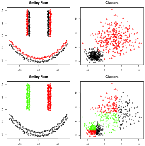
Figure 10: These plots highlight how the distribution of points in one space is related to the distribution of points in the other. Looking at the plots on the left in Figure 10, each of the three clusters is in fact composed of two subclusters. Likewise, each of the two clusters in the plots on the right are composed of three subclusters.

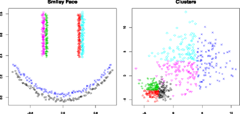
Figure 11: In this plot each of the six underlying subgroups shown in Figure 10 is highlighted.

The underlying structure between these spaces is illustrated in Figure 10. The top row of plots tells us about how the distribution of points on the right (cluster space) relates to the distribution of points on the left (smiley face space). The bottom set of plots tells us about how the distribution of points on the left is related to distribution of points on the right.

If we were to look at the two spaces as marginal distributions, there is a distinct impression of the three clusters in the left, and two in the right. The joint distribution, however, has six distinct groups. Looking at the plots on the left in Figure 10, each of the three clusters is in fact composed of two subclusters. Likewise, each of the two clusters in the plots on the right are composed of three subclusters. Ideally, the projections onto the KCCA directions would identify each of these six groups, shown in Figure 11.

Using an RBF kernel with $\sigma=1/2$ we look at the first five canonical directions. Ideally, what we would see is a separation of each of the groups as well as a strong alignment between each of the spaces. What we find looking at Figure 12, a scatter plot matrix of the first five kernel canonical variates (KCV), is that while the leading correlations are large (0.98, 0.97, 0.95, 0.80, 0.75), we are not able to find the structure in the data we were looking for, that is, separating out the six groups (with each of the colors corresponding to one of the six groups). Note that only the projections in the smiley face space are shown since the cluster space projections look essentially the same.

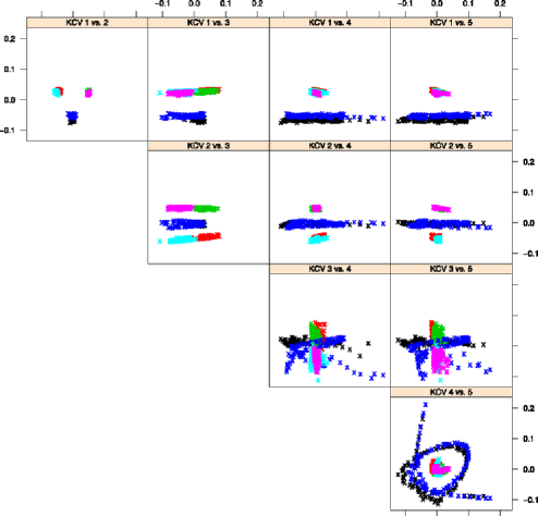
Figure 12: Scatterplot matrix of the first five KCCA direction vectors for the data shown in Figure 9. Each of the colors in this plot corresponds to one of the six underlying subpopulation in the data (see Figure 10 for details).

In the context of the protein–ligand matching problem this type of situation presents a potential problem. Suppose a new point, say in the space with the smiley face, is projected into KCCA space. As can be seen in Figure 12, there is a great deal of overlap between each of the six subgroups in the projected space. In particular note that each of the overlapped groups is composed of, respectively, the left eye, right eye and mouth. The reason this type of behavior presents a problem is that each of the eyes and the mouth are actually composed of two different subpopulations where each of the populations correspond to very different groups in the space with the two clusters. So while we may be able to accurately predict the location of a new point in KCCA space the interpretation of its surrounding neighbors may not be so meaningful.

4 Indefinite kernel canonical correlation analysis

A potential shortcoming of standard KCCA, which was illustrated in the example presented in Figure 9, is that standard positive definite kernels can be limited in their ability to capture nonstandard heterogeneous behavior in the data. A more general class of kernels which is better suited to handle this type of behavior takes the form

$$K(\mathbf{x}_{i},\mathbf{x}_{j})=\cases{\displaystyle w(\mathbf{x}_{i},\mathbf{x}_{j}),&\quad if $\mathbf{x}_{j}\in N(\mathbf{x}_{i})$,\cr 0,&\quad otherwise.}$$ (6)

Here $N(\mathbf{x})$ denotes some neighborhood of the observation $\mathbf{x}$, such as a $k(\in\mathbb{Z}_{+})$ nearest neighborhood or a fixed radius $\varepsilon(>0)$-neighborhood. Kernels of this form restrict attention to the local structure of the data and allow for a flexible definition of similarity.

Our motivation for considering this class of kernels in the context of the protein–ligand matching problem is the following. In the RLP800 dataset there are approximately 150 important subgroups in the data. These subgroups correspond to unique proteins, or more specifically their binding pockets, which typically have three or four different conformations specific to a particular ligand. Exploitation of this group structure in the data can help improve prediction. This can be accomplished by using a “local kernel” function that allows us to capture these groups more readily than, say, the RBF kernel. The intuition here follows from the example presented in Section 3.3 where we saw that the type of groups that an RBF kernel will be able to find will be dictated by the choice of the bandwidth parameter $\sigma$. The local kernel overcomes this by adjusting locally to the data. By adjusting to the data locally it is better able to exploit this group structure.

In summary, given a new protein, its projection in this local kernel CCA space will be more likely to fall into a group of similar proteins. Then, as before, the goal is that the ligands associated with this group of proteins provide an accurate representation of the ligand we are trying to predict.

This improved performance exploiting group structure in the data comes at some price. In particular, the problem encountered with this class of kernels is that they are frequently indefinite (see the discussion following Definition 4.1). As a result of the indefiniteness, many of the properties and optimality guarantees no longer hold.

Indefinite kernels have recently gained increased interest [Ong, Canu and Smola (2004a), Haasdonk (2005), Chen and Ye (2008), Luss and d’Aspremont (2008)] where, rather than defining $K$ to be a function defined in a RKHS, $K$ is defined in a space characterized by an indefinite inner product called a Krein space. In Section 4.1 we provide an overview of some of the definitions and theoretical results about Krein spaces [following the discussion of Ong, Canu and Smola (2004a)].

Before discussing IKCCA, we will need to provide some definitions and theorems related to indefinite inner product spaces, that is, Krein spaces [more details can be found in Ong, Canu and Smola (2004a)].

4.1 Indefinite kernels

Definition 4.1 ((Inner product)).

Let $\mathcal{K}$ be a vector space on the scalar field. An inner product $\langle\cdot,\cdot\rangle_{\mathcal{K}}$ on $\mathcal{K}$ is a bilinear form where for all $f,g,h\in\mathcal{K}$, $\alpha\in\mathbb{R}$:

• $\langle f,g\rangle_{\mathcal{K}}=\langle g,f\rangle_{\mathcal{K}}$;

• $\langle\alpha f+g,h\rangle_{\mathcal{K}}=\alpha\langle f,h\rangle_{\mathcal{K}}+\langle g,h\rangle_{\mathcal{K}}$;

• $\langle f,g\rangle_{\mathcal{K}}=0$ for all $g\in\mathcal{K}$ implies $\Rightarrow f=0$.

The importance of $\mathcal{K}$ being a vector space on a scalar field is that it allows for a flexible definition of an inner product (i.e., the scalar in one of the dimensions could be complex or negative as we will see below). An inner product is said to be positive if for all $f\in\mathcal{K}$, $\langle f,f\rangle_{\mathcal{K}}\geq 0$. It is called a negative inner product, if for all $f\in\mathcal{K}$, $\langle f,f\rangle_{\mathcal{K}}\leq 0$. An inner product is called indefinite if it is neither strictly positive nor strictly negative.

Remark 4.1.

To illustrate how indefinite inner products arise in the context of our problem, consider the following. Suppose we have a symmetric kernel function $K$, which is indefinite, the implication of this is that the resulting kernel matrix $\mathbf{K}=\{K_{ij}\}_{i=1}^{n}$ is indefinite and that it therefore contains positive and negative eigenvalues. Let $\mathbf{K}=\mathbf{U}\bolds{\Lambda}\mathbf{U}^{T}$ be the eigendecomposition of $\mathbf{K}$, where $\mathbf{U}$ are the eigenvectors and $\bolds{\Lambda}$ is the diagonal matrix of eigenvalues starting with the $p$ positive eigenvalues, followed by the $q$ negative ones and the $n-p-q$ eigenvalues equal to 0. To see how $\mathbf{K}$ can be interpreted as a matrix composed of inner products in this indefinite inner product space consider the following representation of its eigendecomposition:

$$\mathbf{K}=\mathbf{U}|\bolds{\Lambda}|^{{1}/{2}}\operatorname{diag}(\mathbf{1}_{p},-\mathbf{1}_{q},\mathbf{0}_{n-p-q})|\bolds{\Lambda}|^{{1}/{2}}\mathbf{U}^{T}.$$

Let $\mathbf{M}=\operatorname{diag}(\mathbf{1}_{p},-\mathbf{1}_{q})$ and $\bolds{\Phi}$ be equal to the first $p+q$ columns of $\mathbf{U}|\bolds{\Lambda}|^{{1}/{2}}$. Define the $i$th row of $\bolds{\Phi}$ to be equal to

$$\Phi_{i}=(\underbrace{\phi_{i,1},\ldots,\phi_{i,p}}_{=\Phi_{i}^{+}},\underbrace{\phi_{i,p+1},\ldots,\phi_{i,p+q}}_{=\Phi_{i}^{-}}).$$

We then have a kernel matrix composed of elements

$$K_{ij} = \Phi_{i}^{T}\mathbf{M}\Phi_{j}$$

$$= (\Phi_{i}^{+})^{T}\Phi_{j}^{+}-(\Phi_{i}^{-})^{T}\Phi_{j}^{-}$$

$$= \langle\Phi_{i},\Phi_{j}\rangle_{\mathcal{H}_{+}}-\langle\Phi_{i},\Phi_{j}\rangle_{\mathcal{H}_{-}}$$

$$= \langle\Phi_{i},\Phi_{j}\rangle_{\mathcal{K}}.$$

From (4.1) we can see that unlike PSD kernels where $\mathbf{a}^{T}\mathbf{K}\mathbf{a}\geq 0$ for any $\mathbf{a}\in\mathbb{R}^{n}$, with indefinite kernels $\mathbf{a}^{T}\mathbf{K}\mathbf{a}$ can take on any value, making optimization over such a quantity challenging.

Despite this difference, many of the properties that hold for reproducing kernel Hilbert spaces (RKHS), such as (and perhaps most importantly) the reproducing property [Schölkopf and Smola (2002)], also hold for these indefinite inner product spaces [see Ong, Canu and Smola (2004b) for details]. The key difference lies in the fact that rather than minimizing (maximizing) a regularized risk functional, as in the RKHS setting, the corresponding optimization problem becomes that of finding a stationary point of a similar risk functional.

4.2 Indefinite kernel canonical correlation

Section 4.1 provided some insight into the challenges that arise from dealing with indefinite kernels. In particular, Remark 4.1 points to the fact that the solution that we find may not be globally, or even locally, optimal (as it may be a saddle point). The form of the IKCCA problem we present in this section is motivated by the discussion of the previous section and the works of Ong, Canu and Smola (2004b) and Luss and d’Aspremont (2008). In particular, the addition of a stabilizing function on the indefinite inner product $\langle f,f\rangle_{\mathcal{K}}$ as discussed in Ong, Canu and Smola (2004b) led us to consider introducing a constraint on the behavior on the indefinite kernels matrix itself.

In the following, let $\|\cdot\|_{F}$ denote the Frobenius norm. Define $\mathbf{M}\succeq 0$ to mean that the matrix $\mathbf{M}$ is positive semi-definite and let $\lambda_{X},\lambda_{Y}\in\mathbb{R}^{+}\cup\infty$ be tuning parameters (discussed in more detail later this section). Here $\mathbf{K}_{X}^{0}$ and $\mathbf{K}_{Y}^{0}$ are the (potentially) indefinite kernels and $\mathbf{K}_{X}$ and $\mathbf{K}_{Y}$ will be the positive semi-definite approximations of these kernels. With this notation in mind, we now define the IKCCA optimization problem:

$$\rho_{\mathcal{H}}=\max_{\mathbf{A}_{X},\mathbf{A}_{Y}}\min_{\mathbf{K}_{X},\mathbf{K}_{Y}}\operatorname{Tr}(\mathbf{A}_{X}^{T}\mathbf{K}_{X}\mathbf{K}_{Y}\mathbf{A}_{Y})+\lambda_{X}\|\mathbf{K}_{X}-\mathbf{K}_{X}^{0}\|_{F}^{2}$$

$$\hphantom{\rho_{\mathcal{H}}=}{}+\lambda_{Y}\|\mathbf{K}_{Y}-\mathbf{K}_{Y}^{0}\|_{F}^{2},$$

subject to

$$\mathbf{A}_{X}^{T}\mathbf{K}_{X}^{2}\mathbf{A}_{X}+\kappa\mathbf{A}_{X}^{T}\mathbf{A}_{X}=\mathbf{I}_{n},$$

$$\mathbf{A}_{Y}^{T}\mathbf{K}_{Y}^{2}\mathbf{A}_{Y}+\kappa\mathbf{A}_{Y}^{T}\mathbf{A}_{Y}=\mathbf{I}_{n},$$ (8)

$$(\alpha_{X}^{i})^{T}\mathbf{K}_{X}\mathbf{K}_{Y}\alpha_{Y}^{j}=0\qquad\mbox{for }i\neq j,i,j=1,\ldots,n,$$

$$\mathbf{K}_{X}\succeq\mathbf{0},$$

$$\mathbf{K}_{Y}\succeq\mathbf{0},$$

where $\mathbf{A}_{X}=(\alpha_{X}^{1},\ldots,\alpha_{X}^{n})$ and $\mathbf{A}_{Y}=(\alpha_{Y}^{1},\ldots,\alpha_{Y}^{n})$. Note that this optimization problem and the KCCA optimization problem are only equivalent when the kernel matrices $\mathbf{K}_{X}^{0}$ and $\mathbf{K}_{Y}^{0}$ are positive semi-definite (see the Supplementary Material [Samarov et al. (2011)] for details on the equivalency between the optimization problem in (4.2) and (3.2) and a proof of Theorem 4.3).

Theorem 4.2

Letting $\lambda_{X},\lambda_{Y}\rightarrow\infty$, the optimization problem in $(\ref{sccaoptim})$ is concave in $\alpha_{X}^{i}$ and $\alpha_{Y}^{i}$, $i=1,\ldots,n,$ and convex in $\mathbf{K}_{X}$ and $\mathbf{K}_{Y}$.

See the Supplementary Material for a proof. Let $(\mathbf{X})_{+}$ denote the positive part of the matrix $\mathbf{X}$, that is, $(\mathbf{X})_{+}=\sum_{i}\max(0,\lambda_{i})\mathbf{v}_{i}\mathbf{v}_{i}^{T}$, where $\lambda_{i}$ and $\mathbf{v}_{i}$ are $i$th eigenvalue–eigenvector pair of the matrix $\mathbf{X}$. With this in mind, we have the following theorem.

Theorem 4.3

Letting $\lambda_{X},\lambda_{Y}\rightarrow\infty$, and given the optimization problem in $(\ref{sccaoptim})$ the optimal values for $\mathbf{K}_{X}$ and $\mathbf{K}_{Y}$ are given by

$$\mathbf{K}_{X} = (\mathbf{K}_{X}^{0})_{+},$$

$$\mathbf{K}_{Y} = (\mathbf{K}_{Y}^{0})_{+}.$$

The proof of Theorem 4.3 makes use of the following lemma. Let $\mathbf{M}_{0}\in\mathbb{R}^{n\times n}$ be a known, square, not necessarily positive-definite matrix, and $\mathbf{M}\in\mathbb{R}^{n\times n}$ a square, unknown matrix, then:

Lemma 4.1.

The solution to the optimization problem

$$\operatorname{arg}\min_{\mathbf{M}\succeq 0}\|\mathbf{M}-\mathbf{M}_{0}\|^{2}_{F},$$

is

$$\mathbf{M}=(\mathbf{M}_{0})_{+}.$$

The proofs of Theorem 4.3 and Lemma 4.1 can be found in the Supplemen- tary Material.

Points $\mathbf{x}\in\mathbb{R}^{d_{X}}$ and $\mathbf{y}\in\mathbb{R}^{d_{Y}}$ are projected onto their first $p$ canonical directions as follows: first compute their kernelization, using the indefinite kernel functions $K_{X}^{0}$ and $K_{Y}^{0}$,

$$K_{X}^{0}(\mathbf{x},\cdot) = (K_{X}^{0}(\mathbf{x},\mathbf{x}_{1}),\ldots,K_{X}^{0}(\mathbf{x},\mathbf{x}_{n}))^{T},$$

$$K_{Y}^{0}(\mathbf{x},\cdot) = (K_{Y}^{0}(\mathbf{y},\mathbf{y}_{1}),\ldots,K_{Y}^{0}(\mathbf{y},\mathbf{y}_{n}))^{T}.$$

Then calculate

$$K_{X}^{0}(\mathbf{x},\cdot)\mathbf{A}_{X}^{p},$$

$$K_{Y}^{0}(\mathbf{y},\cdot)\mathbf{A}_{Y}^{p},$$

where $\mathbf{A}_{X}^{p}=(\alpha_{X}^{1},\ldots,\alpha_{X}^{p})$ and $\mathbf{A}_{Y}^{p}=(\alpha_{Y}^{1},\ldots,\alpha_{Y}^{p})$.

4.3 Toy example 3: KCCA challenge (motivating IKCCA)

We now return to the example in Section 3.3 using the kernel defined in (6) with weights (10). Note that this kernel is closely related to the Normalized Graph Laplacian (NGL) kernel used in Spectral Clustering; see von Luxburg (2007) for an overview of Spectral Clustering methods. From Figure 13, it can be seen that we are now able to capture the underlying structure of the data, identifying each of the six subpopulations:

$$a_{ij}=\cases{\displaystyle\exp\biggl{\{}-\frac{1}{2\sigma_{ij}}\|\mathbf{x}_{i}-\mathbf{x}_{j}\|^{2}\biggr{\}},&\quad if $\mathbf{x}_{j}\in N_{k}(\mathbf{x}_{i})$,\cr\displaystyle 0,&\quad otherwise,}$$

and

$$w_{ij}=\frac{a_{ij}}{\sqrt{\sum_{i^{\prime}}a_{i^{\prime}j}}\sqrt{\sum_{j^{\prime}}a_{ij^{\prime}}}}.$$ (10)

Here $N_{k}(\mathbf{x}_{i})$ is the symmetric $k$-neighborhood of the point $\mathbf{x}_{i}$ [i.e., if $\mathbf{x}_{j}\in N_{k}(\mathbf{x}_{i})$ then $\mathbf{x}_{i}\in N_{k}(\mathbf{x}_{j})$] and

$$\sigma_{ij}^{2}=\|\mathbf{x}_{i}-\mathbf{x}_{i}^{k}\|\|\mathbf{x}_{j}-\mathbf{x}_{j}^{k}\|,$$

where $\mathbf{x}_{i}^{k}$ is the $k$th neighbor of the point $\mathbf{x}_{i}$.

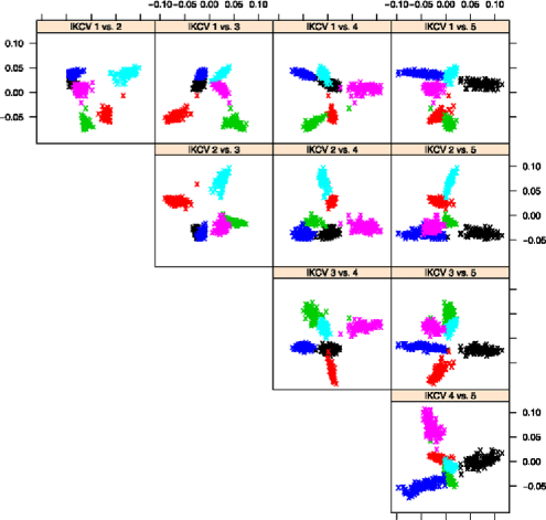
Figure 13: Continuation from the example in Section 4.3. This is a scatter plot matrix of the projections onto the first five IKCCA variates (IKCV) using the kernel in (6) with weights (10). Unlike the projections shown in Figure 12, here we are able to separate out the six groups.

Looking at plots of the first four eigenvectors (Figures 14 and 15) in both the smiley face space and the cluster space, we can see how the behavior of the eigenvectors causes the segmentation of the data that we observe in Figure 13. First, we discuss how these figures are generated and then what it is they are telling us. [(3)]

Generate an equally spaced dimensional grid spanning the range of values in each space.

Calculate the kernel representation and projection of each grid point into IKCCA space.

Use the projected values to assign color intensities to each point in the grid of each space (darker for negative values, lighter for positive values).

Plot the grid and for each point using the colors calculated from the previous step. The important thing to note in both of these figures is the distribution of positive and negative projected values and how these are driving the segmentation, which we observe in Figure 13. For example, in Figure 14 the first canonical variate segments out one of the faces (red) from the other (blue).

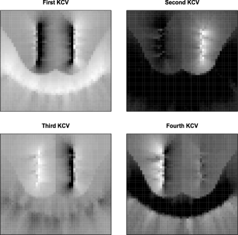
Figure 14: A plot of the first four indefinite kernel canonical direction vectors in the smiley face space from the example in Section 4.3 using the kernel in (6) with weights (10). These plots allow us to visualize how the canonical vectors separate out each of the clusters.

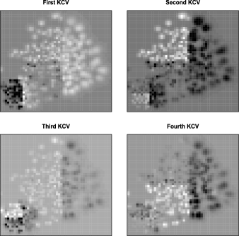
Figure 15: A plot of the first four indefinite kernel canonical directions vectors in the cluster space from the example in Section 4.3 using the kernel in (6) with weights (10).

5 Ligand prediction

5.1 Prediction

Let us define the projected values of the observations in protein and ligand space onto their first $p$ canonical vectors as $\mathbf{x}_{i,p}^{w}=(\mathbf{w}_{X}^{1},\ldots,\mathbf{w}_{X}^{p_{X}})^{T}\mathbf{x}_{i}$, $\mathbf{x}_{i,p}^{w}\in\mathbb{R}^{p}$, and $\mathbf{y}_{i,p}^{w}=(\mathbf{w}_{Y}^{1},\ldots,\mathbf{w}_{Y}^{p_{Y}})^{T}\mathbf{y}_{i}$, $\mathbf{y}_{i,p}^{w}\in\mathbb{R}^{p}$, $i=1,\ldots,n$. The predicted value of $\mathbf{y}^{w}_{\mathrm{new},p}$ is calculated as follows [using a modification of the LLE algorithm of Saul and Roweis (2003)]: [(3)]

Compute the $k$ neighbors of the data point $\mathbf{x}^{w}_{\mathrm{new},p}$ (the projected value of $\mathbf{x}_{\mathrm{new}}$ into canonical correlation space). Define $N_{k}(\mathbf{x})$ to be the $k$ nearest neighbors of the point $\mathbf{x}$.

Compute weights $\beta_{\mathrm{new},j}$ that best reconstruct the data point $\mathbf{x}^{w}_{\mathrm{new},p}$ from its neighbors, minimizing the cost

$$L(\beta_{\mathrm{new}})=\biggl{(}\mathbf{x}^{w}_{\mathrm{new},p}-\sum_{j\dvtx\mathbf{x}_{j}\in N_{k}(\mathbf{x}^{w}_{\mathrm{new},p})}\beta_{\mathrm{new},j}\mathbf{x}^{w}_{j,p}\biggr{)}^{2},$$

subject to (11)

$$\sum_{j\dvtx\mathbf{x}_{j}\in N_{k}(\mathbf{x}^{w}_{\mathrm{new},p})}\beta_{\mathrm{new},j}=1.$$

The new observation is then calculated as

$$\hat{\mathbf{y}}^{w}_{\mathrm{new},p}=\sum_{j\dvtx\mathbf{x}_{j}\in N_{k}(\mathbf{x}^{w}_{\mathrm{new},p})}\beta_{\mathrm{new},j}\mathbf{y}^{w}_{j,p}.$$

Recall that CCA finds directions which best align two spaces. Thus, assuming that directions $\mathbf{w}_{X}^{i}$ and $\mathbf{w}_{Y}^{i}$, $i=1,\ldots,p$, have been found such that the correlation between spaces is strong, using the weights $\beta_{\mathrm{new},j}$ found in protein space should provide a reliable estimate of $\mathbf{y}^{w}_{\mathrm{new},p}$.

5.2 Tuning parameter selection

Values for the tuning parameters, $\kappa=\kappa_{X}=\kappa_{Y}$ (the regularization parameter), $p=p_{X}=p_{Y}$ (the number of dimensions we are projecting into), $k_{\mathrm{LLE}}$ (the neighborhood for the LLE-based prediction), $\sigma$ (for the RBF kernel) and $k_{\mathrm{NGL}}$ (for the NGL kernel) are found by searching over a suitable $3\times 3\times 3\times 3$ grid for each. The final set of parameters are selected based on which produces the lowest average rank (discussed in Section 1).

[id=samarovTech2010] Local kernel canonical correlation analysis with application to virtual drug screening [doi]10.1214/11-AOAS472SUPP [url]http://lib.stat.cmu.edu/aoas/472/supplement.pdf .pdf Drug discovery is the process of identifying compounds which have potentially meaningful biological activity. A major challenge that arises is that the number of compounds to search over can be quite large, sometimes numbering in the millions, making experimental testing intractable. For this reason computational methods are employed to filter out those compounds which do not exhibit strong biological activity. This filtering step, also called virtual screening reduces the search space, allowing for the remaining compounds to be experimentally tested.
In this paper we propose several novel approaches to the problem of virtual screening based on Canonical Correlation Analysis (CCA) and on a kernel based extension. Spectral learning ideas motivate our proposed new method called Indefinite Kernel CCA (IKCCA). We show the strong performance of this approach both for a toy problem as well as using real world data with dramatic improvements in predictive accuracy of virtual screening over an existing methodology.

References

- Abraham (2003) {bbook}[auto:STB—2011/08/01—08:01:26] \bauthor\bsnmAbraham, \bfnmD. J.\binitsD. J. (\byear2003). \btitleBurger’s Medicinal Chemistry and Drug Discovery, \bedition6th ed. \bseriesDrug Discovery \bvolume1. \bpublisherWiley, \baddressNew York. \bptokimsref \endbibitem
- Anderson (2003) {bbook}[mr] \bauthor\bsnmAnderson, \bfnmT. W.\binitsT. W. (\byear2003). \btitleAn Introduction to Multivariate Statistical Analysis, \bedition3rd ed. \bpublisherWiley-Interscience, \baddressHoboken, NJ. \bidmr=1990662 \bptokimsref \endbibitem
- Bach and Jordan (2002) {barticle}[mr] \bauthor\bsnmBach, \bfnmFrancis R.\binitsF. R. and \bauthor\bsnmJordan, \bfnmMichael I.\binitsM. I. (\byear2002). \btitleKernel independent component analysis. \bjournalJ. Mach. Learn. Res. \bvolume3 \bpages1–48. \biddoi=10.1162/153244303768966085, issn=1532-4435, mr=1966051 \bptnotecheck year\bptokimsref \endbibitem
- Chen and Ye (2008) {bincollection}[auto:STB—2011/08/01—08:01:26] \bauthor\bsnmChen, \bfnmJ.\binitsJ. and \bauthor\bsnmYe, \bfnmJ.\binitsJ. (\byear2008). \btitleTraining svm with indefinite kernels. In \bbooktitleICML’08: Proceedings of the 25th International Conference on Machine Learning \bpages136–143. \bpublisherACM Press, \baddressNew York. \bptokimsref \endbibitem
- Daylight (2004) {bmisc}[auto:STB—2011/08/01—08:01:26] \borganizationDaylight (\byear2004). \bhowpublishedWorld drug index. Available at www.daylight.com. \bptokimsref \endbibitem
- Haasdonk (2005) {barticle}[auto:STB—2011/08/01—08:01:26] \bauthor\bsnmHaasdonk, \bfnmB.\binitsB. (\byear2005). \btitleFeature space interpretation of svms with indefinite kernels. \bjournalIEEE Transaction on Pattern Analysis and Machine Intelligence \bvolume27 \bpages482–492. \bptokimsref \endbibitem
- Hardoon and Shawe-Taylor (2008) {bmisc}[auto:STB—2011/08/01—08:01:26] \bauthor\bsnmHardoon, \bfnmD.\binitsD. and \bauthor\bsnmShawe-Taylor, \bfnmJ.\binitsJ. (\byear2008). \bhowpublishedSparse canonical correlation analysis. Technical report, PASCAL EPrints [http://eprints.pascal-network.org/perl/oai2] (United Kingdom). Available at http://eprints.pascal-network.org/archive/ 00004673/. \bptokimsref \endbibitem
- Hardoon, Szedmak and Shawe-Taylor (2004) {barticle}[pbm] \bauthor\bsnmHardoon, \bfnmDavid R.\binitsD. R., \bauthor\bsnmSzedmak, \bfnmSandor\binitsS. and \bauthor\bsnmShawe-Taylor, \bfnmJohn\binitsJ. (\byear2004). \btitleCanonical correlation analysis: An overview with application to learning methods. \bjournalNeural Comput. \bvolume16 \bpages2639–2664. \biddoi=10.1162/0899766042321814, issn=0899-7667, pmid=15516276 \bptokimsref \endbibitem
- Hotelling (1936) {barticle}[auto:STB—2011/08/01—08:01:26] \bauthor\bsnmHotelling, \bfnmH.\binitsH. (\byear1936). \btitleRelations between two sets of variates. \bjournalBiometrika \bvolume28 \bpages321–377. \bptokimsref \endbibitem
- Kitchen et al. (2004) {bmisc}[auto:STB—2011/08/01—08:01:26] \bauthor\bsnmKitchen, \bfnmD. B.\binitsD. B., \bauthor\bsnmDecornez, \bfnmH.\binitsH., \bauthor\bsnmFurr, \bfnmJ. R.\binitsJ. R. and \bauthor\bsnmBajorath, \bfnmJ.\binitsJ. (\byear2004). \bhowpublishedDocking and scoring in virtual screening for drug discovery: Methods and application. Nature Reviews Drug Discovery 3 935–949. \bptokimsref \endbibitem
- Kuss and Graepel (2002) {bmisc}[auto:STB—2011/08/01—08:01:26] \bauthor\bsnmKuss, \bfnmM.\binitsM. and \bauthor\bsnmGraepel, \bfnmT.\binitsT. (\byear2002). \bhowpublishedThe geometry of kernel canonical correlation analysis. Technical report, Max Planck Institute for Biological Cybernetics, Tubingen, Germany. \bptokimsref \endbibitem
- Lai and Fyfe (2000) {barticle}[pbm] \bauthor\bsnmLai, \bfnmP. L.\binitsP. L. and \bauthor\bsnmFyfe, \bfnmC.\binitsC. (\byear2000). \btitleKernel and nonlinear canonical correlation analysis. \bjournalInt. J. Neural. Syst. \bvolume10 \bpages365–377. \bidissn=0129-0657, pmid=11195936 \bptokimsref \endbibitem
- Luss and d’Aspremont (2008) {bmisc}[auto:STB—2011/08/01—08:01:26] \bauthor\bsnmLuss, \bfnmR.\binitsR. and \bauthor\bsnmd’Aspremont, \bfnmA.\binitsA. (\byear2008). \bhowpublishedSupport vector machine classification with indefinite kernels. CoRR abs/0804.0188. \bptokimsref \endbibitem
- Oloff et al. (2006) {barticle}[pbm] \bauthor\bsnmOloff, \bfnmScott\binitsS., \bauthor\bsnmZhang, \bfnmShuxing\binitsS., \bauthor\bsnmSukumar, \bfnmNagamani\binitsN., \bauthor\bsnmBreneman, \bfnmCurt\binitsC. and \bauthor\bsnmTropsha, \bfnmAlexander\binitsA. (\byear2006). \btitleChemometric analysis of ligand receptor complementarity: Identifying complementary ligands based on receptor information (CoLiBRI). \bjournalJ. Chem. Inf. Model. \bvolume46 \bpages844–851. \biddoi=10.1021/ci050065r, issn=1549-9596, mid=NIHMS144502, pmcid=2755506, pmid=16563016 \bptokimsref \endbibitem
- Ong, Canu and Smola (2004a) {bmisc}[auto:STB—2011/08/01—08:01:26] \bauthor\bsnmOng, \bfnmC. S.\binitsC. S., \bauthor\bsnmCanu, \bfnmS.\binitsS. and \bauthor\bsnmSmola, \bfnmA. J.\binitsA. J. (\byear2004a). \bhowpublishedLearning with non-positive kernels. In Proc. of the 21st International Conference on Machine Learning (ICML) 639–646. \bptokimsref \endbibitem
- Ong, Canu and Smola (2004b) {bmisc}[auto:STB—2011/08/01—08:01:26] \bauthor\bsnmOng, \bfnmC. S.\binitsC. S., \bauthor\bsnmCanu, \bfnmS.\binitsS. and \bauthor\bsnmSmola, \bfnmA. J.\binitsA. J. (\byear2004b). \bhowpublishedLearning with non-positive kernels. In Proc. of the 21st International Conference on Machine Learning (ICML) 639–646. \bptokimsref \endbibitem
- Parkhomenko (2008) {bmisc}[auto:STB—2011/08/01—08:01:26] \bauthor\bsnmParkhomenko, \bfnmE.\binitsE. (\byear2008). \bhowpublishedSparse canonical correlation analysis. Ph.D. thesis, Dept. Biostatistics, Univ. Toronto. \bptokimsref \endbibitem
- Samarov et al. (2011) {bmisc}[auto:STB—2011/08/01—08:01:26] \bauthor\bsnmSamarov, \bfnmDaniel\binitsD., \bauthor\bsnmMarron, \bfnmJ. S.\binitsJ. S., \bauthor\bsnmLiu, \bfnmYufeng\binitsY., \bauthor\bsnmGrulke, \bfnmChristopher\binitsC. and \bauthor\bsnmTropsha, \bfnmAlexander\binitsA. (\byear2011). \bhowpublishedSupplement to “Local kernel canonical correlation analysis with application to virtual drug screening.” DOI:10.1214/11-AOAS472SUPP. \endbibitem
- Saul and Roweis (2003) {barticle}[mr] \bauthor\bsnmSaul, \bfnmLawrence K.\binitsL. K. and \bauthor\bsnmRoweis, \bfnmSam T.\binitsS. T. (\byear2003). \btitleThink globally, fit locally: Unsupervised learning of low dimensional manifolds. \bjournalJ. Mach. Learn. Res. \bvolume4 \bpages119–155. \biddoi=10.1162/153244304322972667, issn=1532-4435, mr=2050880 \bptnotecheck year\bptokimsref \endbibitem
- Schölkopf and Smola (2002) {bbook}[auto:STB—2011/08/01—08:01:26] \bauthor\bsnmSchölkopf, \bfnmB.\binitsB. and \bauthor\bsnmSmola, \bfnmA. J.\binitsA. J. (\byear2002). \btitleLearning with Kernels. \bpublisherMIT Press, \baddressCambridge, MA. \bptokimsref \endbibitem
- Todeschini and Consonni (2009a) {bmisc}[auto:STB—2011/08/01—08:01:26] \bauthor\bsnmTodeschini, \bfnmR.\binitsR. and \bauthor\bsnmConsonni, \bfnmV.\binitsV. (\byear2009a). \bhowpublishedMolecular Descriptors for Chemoinformatics: Volume I: Alphabetical Listing 1. Wiley, New York. \bptokimsref \endbibitem
- Todeschini and Consonni (2009b) {bmisc}[auto:STB—2011/08/01—08:01:26] \bauthor\bsnmTodeschini, \bfnmR.\binitsR. and \bauthor\bsnmConsonni, \bfnmV.\binitsV. (\byear2009b). \bhowpublishedMolecular Descriptors for Chemoinformatics: Volume II: Appendices, References (Methods and Principles in Medicinal Chemistry) 1. Wiley, New York. \bptokimsref \endbibitem
- Tropsha (2003) {bbook}[auto:STB—2011/08/01—08:01:26] \bauthor\bsnmTropsha, \bfnmA.\binitsA. (\byear2003). \btitleRecent Trends in Quantitative Structure-Activity Relationships, \bedition6th ed. \bpublisherWiley, \baddressNew York. \bptokimsref \endbibitem
- Vinod (1976) {barticle}[auto:STB—2011/08/01—08:01:26] \bauthor\bsnmVinod, \bfnmH.\binitsH. (\byear1976). \btitleCanonical ridge and econometrics of joint production. \bjournalJ. Econometrics \bvolume4 \bpages147–166. \bptokimsref \endbibitem
- von Luxburg (2007) {barticle}[mr] \bauthor\bparticlevon \bsnmLuxburg, \bfnmUlrike\binitsU. (\byear2007). \btitleA tutorial on spectral clustering. \bjournalStat. Comput. \bvolume17 \bpages395–416. \biddoi=10.1007/s11222-007-9033-z, issn=0960-3174, mr=2409803 \bptokimsref \endbibitem
- Wang et al. (2004) {barticle}[pbm] \bauthor\bsnmWang, \bfnmRenxiao\binitsR., \bauthor\bsnmFang, \bfnmXueliang\binitsX., \bauthor\bsnmLu, \bfnmYipin\binitsY. and \bauthor\bsnmWang, \bfnmShaomeng\binitsS. (\byear2004). \btitleThe PDBbind database: Collection of binding affinities for protein–ligand complexes with known three-dimensional structures. \bjournalJ. Med. Chem. \bvolume47 \bpages2977–2980. \biddoi=10.1021/jm030580l, issn=0022-2623, pmid=15163179 \bptokimsref \endbibitem
- Warren et al. (2006) {barticle}[pbm] \bauthor\bsnmWarren, \bfnmGregory L.\binitsG. L., \bauthor\bsnmAndrews, \bfnmC. Webster\binitsC. W., \bauthor\bsnmCapelli, \bfnmAnna-Maria\binitsA.-M., \bauthor\bsnmClarke, \bfnmBrian\binitsB., \bauthor\bsnmLaLonde, \bfnmJudith\binitsJ., \bauthor\bsnmLambert, \bfnmMillard H.\binitsM. H., \bauthor\bsnmLindvall, \bfnmMika\binitsM., \bauthor\bsnmNevins, \bfnmNeysa\binitsN., \bauthor\bsnmSemus, \bfnmSimon F.\binitsS. F., \bauthor\bsnmSenger, \bfnmStefan\binitsS., \bauthor\bsnmTedesco, \bfnmGiovanna\binitsG., \bauthor\bsnmWall, \bfnmIan D.\binitsI. D., \bauthor\bsnmWoolven, \bfnmJames M.\binitsJ. M., \bauthor\bsnmPeishoff, \bfnmCatherine E.\binitsC. E. and \bauthor\bsnmHead, \bfnmMartha S.\binitsM. S. (\byear2006). \btitleA critical assessment of docking programs and scoring functions. \bjournalJ. Med. Chem. \bvolume49 \bpages5912–5931. \biddoi=10.1021/jm050362n, issn=0022-2623, pmid=17004707 \bptokimsref \endbibitem
- Witten and Tibshirani (2009) {barticle}[mr] \bauthor\bsnmWitten, \bfnmDaniela M.\binitsD. M. and \bauthor\bsnmTibshirani, \bfnmRobert J.\binitsR. J. (\byear2009). \btitleExtensions of sparse canonical correlation analysis with applications to genomic data. \bjournalStat. Appl. Genet. Mol. Biol. \bvolume8 \bpagesArt. 28, 29. \bidissn=1544-6115, mr=2533636 \bptokimsref \endbibitem
- Witten, Tibshirani and Hastie (2009) {barticle}[pbm] \bauthor\bsnmWitten, \bfnmDaniela M.\binitsD. M., \bauthor\bsnmTibshirani, \bfnmRobert\binitsR. and \bauthor\bsnmHastie, \bfnmTrevor\binitsT. (\byear2009). \btitleA penalized matrix decomposition, with applications to sparse principal components and canonical correlation analysis. \bjournalBiostatistics \bvolume10 \bpages515–534. \biddoi=10.1093/biostatistics/kxp008, issn=1468-4357, pii=kxp008, pmcid=2697346, pmid=19377034 \bptokimsref \endbibitem