Magnetic field amplification during gravitational collapse - Influence of initial conditions on dynamo evolution and saturation

Abstract

We study the influence of initial conditions on the magnetic field amplification during the collapse of a magnetised gas cloud. We focus on the dependence of the growth and saturation level of the dynamo generated field on the turbulent properties of the collapsing cloud. In particular, we explore the effect of varying the initial strength and injection scale of turbulence and the initial uniform rotation of the collapsing magnetised cloud. In order to follow the evolution of the magnetic field in both the kinematic and the nonlinear regime, we choose an initial field strength of $\simeq 1\,\,{\rm\mu G}$ with the magnetic to kinetic energy ratio, $E_{\rm m}/E_{\rm k}\sim 10^{-4}$. Both gravitational compression and the small-scale dynamo initially amplify the magnetic field. Further into the evolution, the dynamo-generated magnetic field saturates but the total magnetic field continues to grow because of compression. The saturation of the small-scale dynamo is marked by a change in the slope of $B/\rho^{2/3}$ and by a shift in the peak of the magnetic energy spectrum from small scales to larger scales. For the range of initial Mach numbers explored in this study, the dynamo growth rate increases as the Mach number increases from $v_{\rm rms}/c_{\rm s}\sim 0.2$ to $0.4$ and then starts decreasing from $v_{\rm rms}/c_{\rm s}\sim 1.0$. We obtain saturation values of $E_{\rm m}/E_{\rm k}=0.2-0.3$ for these runs. Simulations with different initial injection scales of turbulence also show saturation at similar levels. For runs with different initial rotation of the cloud, the magnetic energy saturates at $E_{\rm m}/E_{\rm k}\sim 0.2-0.4$ of the equipartition value. The overall saturation level of the magnetic energy, obtained by varying the initial conditions are in agreement with previous analytical and numerical studies of small-scale dynamo action where turbulence is driven by an external forcing instead of gravitational collapse.

1 Introduction

Magnetic fields are ubiquitous in astrophysical systems and their study forms an active area of research today. Radio observations over the last few decades have revealed that galaxies and galaxy clusters host magnetic fields. The total magnetic field strength in nearby spiral galaxies is $\sim 9-15\,\,{\rm\mu G}$ (Beck & Hoernes, 1996; Beck, 2004) while observations of cluster magnetic fields show that fields are at the $\,{\rm\mu G}$ level, with values up to tens of $\,{\rm\mu G}$ at the center of cooling core clusters (Carilli & Taylor, 2002; Govoni & Feretti, 2004). Recent observations also point to the existence of magnetic fields in the high-redshift universe (Bernet et al., 2008). One plausible mechanism of the origin of such magnetic fields is the dynamo process where energy in the turbulent fluid motions is tapped to amplify the magnetic field. Turbulence is ubiquitous in all astrophysical systems ranging from protostellar accretion disks in individual star forming clouds to the interstellar medium (ISM) in galaxies and possibly also in the gaseous media of galaxy clusters and cosmic filaments. In fluid dynamics, turbulence is described as a flow regime characterised by chaotic motions and involves the cascade of energy from the scale of the largest eddy to the smallest scale eddy. In particular, the small-scale dynamo process (Kazantsev, 1968; Vainshtein, 1982; Schekochihin et al., 2002; Boldyrev & Cattaneo, 2004; Sur et al., 2010; Federrath et al., 2011b; Schober et al., 2011) can lead to rapid amplification of initial seed magnetic fields (see Brandenburg & Subramanian, 2005, for a review). Earlier work by Beck et al. (1994) proposed that such dynamo action is responsible for producing seed magnetic fields for the galactic large-scale dynamo. The same mechanism is found to amplify magnetic fields in galaxy clusters (Dolag et al., 1999; Subramanian et al., 2006; Xu et al., 2009, 2011) and also in the cosmological large-scale structure (Ryu et al., 2008). Mergers during cluster formation can also lead to turbulence and intense random vortical flows (Schindler & Mueller, 1993; Kulsrud et al., 1997; Bryan & Norman, 1998; Miniati et al., 2001; Ricker & Sarazin, 2001; Subramanian et al., 2006) capable of amplifying magnetic fields by the dynamo process (Subramanian et al., 2006).

A potential application of small-scale dynamos concerns the formation of the first stars and the first galaxies where high-resolution simulations have revealed the ubiquity of turbulence in the early Universe suggesting that the primordial gas is highly turbulent (Abel et al., 2002; O’Shea & Norman, 2007; Wise & Abel, 2007; Yoshida et al., 2008; Greif et al., 2008; Turk et al., 2009). This has strong implications for the exponential amplification of magnetic fields by the small-scale dynamo process during the formation of the first stars and in first galaxies (Schleicher et al., 2010; Sur et al., 2010; Federrath et al., 2011b; Turk et al., 2011). High-resolution three-dimensional magnetohydrodynamics (MHD) simulations of collapsing magnetized primordial clouds by Sur et al. (2010) and Federrath et al. (2011b) (hereafter Paper I and II respectively) show that the turbulence is driven by the gravitational collapse on scales of the order of the local Jeans length. This leads to an exponential growth of the magnetic field by random stretching, folding and twisting of the field lines. In the kinematic stage, the dynamo amplification occurs on the eddy-turnover time scale, $t_{\rm ed}=l/v$ where, $l$ and $v$ are the typical turbulent scale and turbulent velocity respectively. In a collapsing magnetized system, field amplification by the turbulent dynamo should occur on a time scale smaller than the free-fall time, $t_{\rm ff}\sim 1/\sqrt{G\,\rho}$ to enable field growth faster than the rate at which gravitational compression would amplify the field (Papers I and II). Here $\rho$ is the total mass density and $G$ is the gravitational constant. We note here that the efficiency of the dynamo process depends on the Reynolds number and is thus related to how well the turbulent motions are resolved in numerical simulations. Higher Reynolds number would yield faster field amplification. Indeed, in the limit of infinite magnetic Prandtl number (i.e., ${\rm Pr}={\rm Rm}/{\rm Re}\rightarrow\infty$) , Schober et al. (2011) find a dependence of the growth rate on ${\rm Re}$,

$$\Gamma\sim f\,{\rm Re}^{(1-\xi)/(1+\xi)}$$ (1)

where $\xi=1/3$ and $f=1.027$ or $\xi=1/2$ and $f=0.184$ for Kolmogorov and Burgers turbulence respectively.

However, the exorbitant computational costs associated with these simulations and the fact that current simulations largely underestimate the growth rate of the dynamo due to the modest Reynolds numbers achievable, restrict following the field evolution to only the kinematic phase of the dynamo. An important question concerning the magnetic field growth by the small-scale dynamo process is at what strength does the dynamo generated field saturate and what is the structure of those fields. Addressing this issue is important to obtain an estimate of the typical saturated field strengths to be expected in the protostellar cores. Saturation of the field is expected to occur when back reactions either via the Lorentz force (Subramanian, 1999; Schekochihin et al., 2004) or via non-ideal MHD effects such as ambipolar diffusion (Pinto & Galli, 2008) become important. In simulations of dynamo action with randomly forced turbulence in a box, saturation of the dynamo is achieved when the magnetic energy associated with the small-scale field grows to a fraction of the equipartition value (Haugen et al., 2004; Schekochihin et al., 2004; Brandenburg & Subramanian, 2005; Federrath et al., 2011a). However, the exact meaning of saturation and saturated field strengths in a self-gravitating system is far from clear. In this case, the magnetic field is amplified by both turbulence and gravitational compression of the field lines. Therefore, saturation in a self-gravitating system involves also the gravitational energy and hence the ratio of magnetic to kinetic energies $E_{\rm m}/E_{\rm k}$, does not converge to a constant value i.e., $E_{\rm m}/E_{\rm k}\sim\rho^{1/3}$ (using the fact that the collapse speed $v(\rho)$ approaches a constant during the collapse (Larson, 1969)). Here, $E_{\rm m}\sim B^{2}\,V$ and $E_{\rm k}\sim\rho\,v^{2}\,V$ with $B$ being the magnetic field, $v,\rho$ and $V$ are the velocity, density and the volume respectively. Thus, we use $B\sim\rho^{2/3}$ to define dynamo saturation in our case.

The dynamo amplification of magnetic fields is driven by turbulent fluid motions. Detailed parameter study of small-scale dynamo action in driven turbulence in a box by Federrath et al. (2011a) show that the growth rate and the saturation level of the dynamo are sensitive to the Mach number and the turbulence injection mechanism. It is therefore crucial to explore how variations in the turbulent properties of a gas cloud influence the small-scale dynamo evolution and saturation in self-gravitating systems. In this spirit, we investigate the effects of environment on the gravitational collapse and magnetic field amplification in this paper. The key questions that we intend to address are the following: how does the collapse, growth and saturation level of the magnetic field depend on the initial strength and injection scale of the turbulent velocity? What information concerning dynamo saturation can be obtained from the spectra of magnetic fields? We also seek to understand the collapse dynamics and the field amplification when the imposed uniform rotation of the cloud is varied. We address these questions using the initial conditions described in Papers I and II focussing on the collapse of a primordial gas cloud.

An important issue when studying such systems is the choice of the initial field strength. The field strengths obtained from either cosmological processes like Inflation or phase transition mechanisms or from astrophysical mechanisms are weak and have large uncertainties (see Grasso & Rubinstein, 2001, for a review). Recent FERMI observations of TeV-blazars by Neronov & Vovk (2010) and Tavecchio et al. (2010) have however reported a lower bound of about $(10^{-15}-10^{-16})\,{\rm Gauss}$ for the primordial field. Numerical simulations starting with such weak values for the initial field strength render it almost impossible to probe the saturation level of the dynamo generated fields due to the $\sim{\rm Re}^{1/2}$ scaling of the magnetic field growth rate (therefore requiring higher numerical resolution) and the high computational costs associated. Therefore, it is reasonable to start with a stronger seed field which allows us to probe the field amplification in both the kinematic and the nonlinear stage of the collapse. In all the simulations presented here, we therefore start with an initial field strength of $\sim 1\,\,{\rm\mu G}$ with a ratio $E_{\rm m}/E_{\rm k}\sim 10^{-4}$ well below equipartition. In this sense, our simulations are to be viewed as controlled numerical experiments focussing on exploring the influence of certain parameters (e.g., the initial strength and injection scale of turbulence) on the collapse and magnetic field amplification.

The paper is organized as follows. The numerical setup, initial conditions and the analysis methods of our simulations are outlined in Section 2. We present the results obtained from each of the three different parameter regimes i.e., varying the initial strength and injection scale of the turbulence, and the amount of initial rotation and in Section 3. Finally, we summarize and discuss the implications of our results in Section 4.

2 Method

To study the complex system involving self-gravity, turbulence and magnetic fields, we resort to high-resolution three-dimensional MHD simulations of a magnetised collapsing cloud using the adaptive-mesh refinement (AMR) technique.

2.1 Numerical setup and initial conditions

The basic numerical setup is adopted from the one reported in Papers I and II. We focus on the gravitational collapse and magnetic field amplification of a dense gas cloud, using a simplified setup, where we assume a polytropic equation of state, $P\propto\rho^{\Gamma}$, which relates the pressure $P$ to the density $\rho$ with an exponent $\Gamma=1.1$ in the density range $\rho\sim(10^{-20}-10^{-14})\,\rm{g}\,\,{\rm cm}^{-3}$. Note that this almost isothermal equation of state is a good representation of the thermal behavior of the primordial gas at the densities considered here (Omukai et al., 2005; Clark et al., 2011). The numerical simulations presented here were performed with the AMR code, FLASH2.5 (Fryxell et al., 2000). We solve the equations of ideal MHD, including self-gravity with a refinement criterion guaranteeing that the Jeans length,

$$\lambda_{\rm J}=\left(\frac{\pi c_{\rm s}^{2}}{G\,\rho}\right)^{1/2}$$ (2)

with sound speed $c_{\rm s}$, the gravitational constant $G$ and the density $\rho$ is always refined with a user defined number of cells. The applicability of ideal MHD in our simulations depends on the strength of the coupling between the gas and magnetic fields in primordial clouds. Work by Maki & Susa (2004, 2007) focussing on detailed models of magnetic energy dissipation via Ohmic and ambipolar diffusion find that the ionization degree is sufficiently high in the primordial clouds to ensure a strong coupling between ions and neutrals, thereby maintaining perfect flux-freezing. This is specifically true for the primordial clouds which we address here. On the other hand, we expect a higher ionization degree and thus a more idealized situation, in the presence of additional radiation backgrounds in the later Universe. However, non-ideal MHD effects may eventually become important at very high densities, as suggested by simulations of contemporary star formation (e.g., Hennebelle & Teyssier, 2008; Duffin & Pudritz, 2009). These effects are not included in the present calculations, but should be the subject of future studies. It is to be noted that since we use ideal MHD, the magnetic Prandtl number in our simulations is $\sim O(1)$. From earlier studies, we recall that the dynamo amplification requires a threshold resolution of about $30$ grid cells per Jeans length (see Papers I and II). Simulations performed with a resolution below 30 grid cells are unable to resolve the dynamo amplification of magnetic fields. We therefore perform simulations resolving the local Jeans length with a minimum of $64$ cells to a maximum of $128$ cells to explore the influence of initial conditions and the saturated field strengths on the small-scale dynamo generated field. We use the new HLL3R scheme for ideal MHD (Waagan et al., 2011), which employs a 3-wave approximate MHD Riemann solver (Bouchut et al., 2007; Waagan, 2009; Bouchut et al., 2010). The MHD scheme preserves physical states (e.g., positivity of mass density and pressure) by construction, and is highly efficient and accurate in modeling astrophysical MHD problems involving turbulence and shocks (Waagan et al., 2011).

Similar to the studies reported in Papers I and II, we model the gas cloud as an overdense Bonnor-Ebert (BE) sphere (Ebert, 1955; Bonnor, 1956) with a core density of $\rho_{\rm BE}=4.68\times 10^{-20}\,\rm{g}\,\,{\rm cm}^{-3}$ at a temperature of $T=300\,{\rm K}$. Since the aim of this study is to investigate the influence of initial conditions on the evolution of the magnetic field, we choose our initial conditions in a way that allows us to perform a controlled numerical experiment. The initial random seed magnetic field of $1\,\,{\rm\mu G}$ with a power-law dependence $P(k)\sim k^{-2}$ was constructed in Fourier space from the magnetic vector potential which automatically guarantees a divergence-free magnetic field. The turbulence is also modeled with an initial random velocity field with the same power-law dependence as for the initial magnetic field. The parameters of the suite of different simulations we perform is summarized in Table 1. The parameters $\alpha$ and $\beta$ quantify the ratio of initial turbulent energy and the rotational energy to the magnitude of the gravitational energy, respectively. Note that extremely high values of $\alpha$ may prevent the cloud from collapsing under its own gravity. Therefore, we choose initial turbulent velocities in the range $v_{\rm rms}\sim 0.2\,c_{\rm s}-4\,c_{\rm s}$ such that $\alpha$ varies from a minimum of $9.3\times 10^{-3}$ to a maximum of $\sim 3.723$. As for the initial injection scale of turbulence, we focus on two cases, one where the initial turbulence peaks on scales of the order of the initial Jeans length of the core ($l_{\rm inj}=0.7\,\lambda_{\rm J}$) and the other where it peaks on scales $l_{\rm inj}=0.17\,\lambda_{\rm J}$. The initial uniform rotation of the cloud is varied from $\beta=0\%$ to $8\%$.

Simulation	Resolution	Initial Turbulent	Initial Injection	Initial turbulence	Initial rotation
Run	$[\#{\rm of\,cells}/\lambda_{\rm J}]$	velocity $[v_{\rm rms}]$	scale $[l_{\rm int}]$	$\alpha=E_{\rm turb}/|E_{\rm grav}|$	$\beta=E_{\rm rot}/|E_{\rm grav}|$
R64M0.2rot0	64	0.2 $c_{\rm s}$	0.7 $\lambda_{\rm J}$	9.30 $\times 10^{-3}$	0%
R64M0.4rot0	64	0.4 $c_{\rm s}$	0.7 $\lambda_{\rm J}$	3.72$\times 10^{-2}$	0%
R64M1.0rot0	64	1.0 $c_{\rm s}$	0.7 $\lambda_{\rm J}$	0.232	0%
R64M2.0rot0	64	2.0 $c_{\rm s}$	0.7 $\lambda_{\rm J}$	0.930	0%
R64M4.0rot0	64	4.0 $c_{\rm s}$	0.7 $\lambda_{\rm J}$	3.723	0%
R64M1.0rot0lj0.17	64	$c_{\rm s}$	0.17 $\lambda_{\rm J}$	0.233	0%
R128M1.0rot0	128	$c_{\rm s}$	0.7 $\lambda_{\rm J}$	0.232	0%
R128M1.0rot4	128	$c_{\rm s}$	0.7 $\lambda_{\rm J}$	0.232	4%
R128M1.0rot8	128	$c_{\rm s}$	0.7 $\lambda_{\rm J}$	0.232	8%
R16M1.0rot4	16	$c_{\rm s}$	0.7 $\lambda_{\rm J}$	0.232	4%

Table 1: Summary of the simulation runs. These fall in three broad categories : Runs with varying amplitude of the initial turbulence (runs R64M0.2rot0 to R64M4.0rot0) followed by a run (R64M1.0rot0lj0.17) with a different injection scale of the initial turbulence. Finally, runs with with different amounts of initial rotation (runs R16M1.0rot4 to R128M1.0rot8).

2.2 Analysis in the collapsing frame of reference

To understand the behavior of the system quantitatively, we need to follow its dynamical contraction in an appropriate frame of reference. First, we note that the physical time scale becomes progressively shorter during the collapse. We therefore define a dimensionless time coordinate $\tau$ (see Papers I and II),

$$\tau=\int\frac{1}{t_{\mathrm{ff}}(t)}\,dt\,,$$ (3)

which is normalized in terms of the local free-fall time,

$$t_{\mathrm{ff}}(t)=\left(\frac{3\pi}{32\,G\rho_{\rm m}(t)}\right)^{1/2},$$ (4)

where $\rho_{\rm m}(t)$ is the mean density in the central Jeans volume, $V_{\mathrm{J}}=4\pi(\lambda_{\rm J}/2)^{3}/3$. If not otherwise stated, we obtain all dynamical quantities of interest within this contracting Jeans volume, which is centered on the position of the maximum density. This approach enables us to study the turbulence and magnetic field amplification in the collapsing frame of reference. We also note that for runs with different initial conditions, like varying degree of initial rotation, it is more meaningful to compare different simulations at the same central density rather than at the same $\tau$. This is because, runs with different initial conditions are in different phases of the collapse at any given $\tau$. Wherever possible, we therefore show plots of physical quantities as a function of the central mean density. With this in mind, we now proceed to discuss the effects of different initial conditions on the gravitational collapse and magnetic field amplification.

3 Results

In this section, we present the results obtained from numerical simulations of magnetic fields in a collapsing environment. We report on the influence of varying the initial strength and injection scale of the turbulence and, the amount of initial rotation on the collapse dynamics and magnetic field amplification of a magnetized gas cloud. We note that there are two main time scales in the problem - the free-fall time, $t_{\rm ff}\sim 1/\sqrt{G\,\rho}$ and the eddy turnover time scale, $t_{\rm ed}=l/v(l)$. For a $k^{-2}$ spectrum which we adopt here, $v(l)\sim l^{1/2}$ and therefore, $t_{\rm ed}\sim l^{1/2}$ on scales smaller than the injection scale. In paper II we showed that the driving scale of turbulence generated during gravitational collapse is of the order of the local Jeans length. Klessen & Hennebelle (2010) show that it is the very process of formation of structures in the Universe on all scales that drives the turbulence. Given our initial core density, (subsection 2.1) and using the fact that turbulence is driven on the local Jeans length ($\lambda_{\rm J}\sim 1.5\,{\rm pc}$ at $\tau=0$) in our simulations, we have $t_{\rm ed}\sim 68.157\,{\rm yr}$ which is much smaller than the initial free-fall time scale $t_{\rm ff}=0.56\,{\rm Myr}$. On a scale $\sim 0.1\,\lambda_{\rm J}$, the eddy turnover time scale is even smaller which demonstrates that significant dynamo action will occur on smaller scales provided such scales are resolved. In addition to the above two time scales, in presence of rotation, there is an additional time scale $t_{\rm rot}\sim\Omega^{-1}$ where $\Omega$ is the angular velocity. For $\beta=8\%$, $t_{\rm rot}\sim 1.38\,{\rm Myr}$.

3.1 Effect of initial turbulence

In this section, we explore the influence of varying the initial rms turbulent velocity of the cloud on the collapse and magnetic field amplification. The ubiquity of turbulence in the cloud core is central to the idea of magnetic amplification by small-scale dynamo action. While subsonic turbulence correspond to typical velocities found in the first star-forming minihalos, supersonic velocities may correspond to more massive systems like the first galaxies (Wise et al., 2008; Greif et al., 2008).

3.1.1 Evolution of the density and the velocity

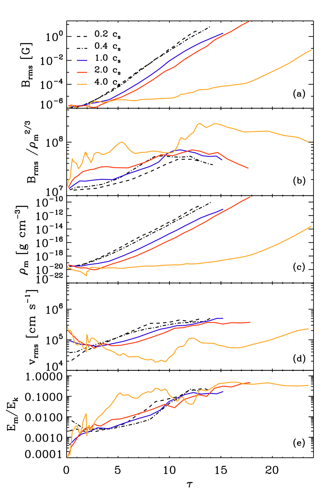
Figure 1: Evolution of the dynamical quantities in the central Jeans volume as a function of $\tau$ for runs with different initial Mach numbers of the turbulence: $v_{\rm rms}/c_{\rm s}=0.2,0.4,1.0,2.0,4.0$. Panel (a) shows the rms magnetic field strength $B_{\rm rms}$, (b) the evolution of $B_{\rm rms}/\rho_{\rm m}^{2/3}$, showing the turbulent dynamo amplification by dividing out the maximum possible amplification due to perfect flux freezing during spherical collapse, (c) the evolution of the mean density $\rho_{\rm m}$, (d) the rms velocity $v_{\rm rms}$, and (e) the ratio of magnetic to kinetic energy, $E_{\rm m}/E_{\rm k}$. All the simulations correspond to a resolution of 64 cells and do not include any initial rotation of the cloud.

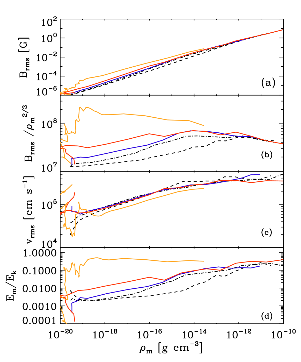
Figure 2: Same as Fig. 1, but now plotted as a function of $\rho_{\rm m}$.

In order to focus on the effects of turbulence, we do not include any ordered rotation of the primordial cloud. Figs. 1 and 2 show the plot of different physical quantities against the normalized time, $\tau$ and the mean density $\rho_{\rm m}$ respectively, for five different values of the initial rms turbulent velocity, $v_{\rm rms}=0.2\,c_{\rm s},0.4\,c_{\rm s},c_{\rm s},2\,c_{\rm s}$ and $4\,c_{\rm s}$. The $\alpha$ parameter corresponding to these values are shown in Table 1. We first focus on the hydrodynamic aspects of these curves, namely the evolution of the mean density (panel c in Fig. 1) and the rms velocity (panels d and c in Figs. 1 and 2 respectively). It turns out that initializing the collapse with different values of the rms turbulent velocity has an effect on how early or late runaway collapse sets in. This is partly due to the fact that the turbulent kinetic energy density prevents the gas from collapsing at the outset for initial transonic and supersonic velocities, while for subsonic velocities, the gas goes into collapse from $\tau\sim 1$. This is shown in the evolutionary behavior of the mean density ($\rho_{\rm m}$). The run with an initial $v_{\rm rms}\sim 4\,c_{\rm s}$ does not undergo runaway collapse till about $\tau\sim 11-12$ because the initial $\alpha$ parameter ($\alpha=3.72$) is high enough to prevent the runaway collapse till the time, the turbulence has decayed. The early stage of the evolution is marked by frequent changes in the rms velocity (panel (c) in Fig. 2) in the density range $(\sim 10^{-20}-10^{-19})\,\rm{g}\,\,{\rm cm}^{-3}$. The evolution of the rms velocity for runs with initial $v_{\rm rms}=1\,c_{\rm s},2\,c_{\rm s}$ is marked by a distinct decay phase till $\tau\sim 3$, after which both curves start to increase as the collapse regenerates the turbulence.

3.1.2 Magnetic field evolution and signatures of dynamo saturation

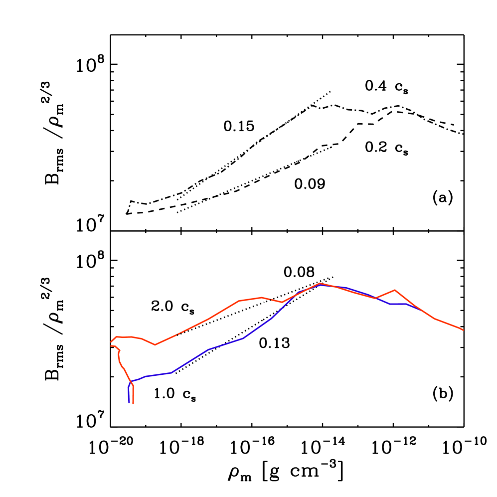
Figure 3: Growth rate of $B_{\rm rms}/\rho_{\rm m}^{2/3}$ for runs with $v_{\rm rms}=0.2\,c_{\rm s},0.4\,c_{\rm s},1.0\,c_{\rm s}$ and $2.0\,c_{\rm s}$. The growth rates for the different runs are computed in the density interval $\rho_{\rm m}\sim 10^{-18}-10^{-14}\,\rm{g}\,\,{\rm cm}^{-3}$ when all the different runs are in identical stages of gravitational collapse. The growth rate of the dynamo generated magnetic field at first increases with increasing subsonic Mach numbers and then starts to decrease in the supersonic regime.

The total magnetic field is amplified by more than 6 orders of magnitude, reaching peak values of $\sim 1\,{\rm G}$ at densities of $\sim 10^{-12}\,\rm{g}\,\,{\rm cm}^{-3}$ evident from panel (a) in Fig. 2. The evolution of the dynamo generated magnetic field is shown in panel (b) of Figs. 1 and 2. Except for the run with $v_{\rm rms}=4\,c_{\rm s}$, the exponential amplification of the magnetic field by the small-scale dynamo continues till $\tau\sim 10$, illustrating the kinematic phase of the dynamo. This phase corresponds to densities up to $\approx 10^{-14}\,\rm{g}\,\,{\rm cm}^{-3}$ for runs with initial $v_{\rm rms}=(0.2-2.0)\,c_{\rm s}$. The exponential phase lasts till $\rho_{\rm m}\sim 10^{-13}\,\rm{g}\,\,{\rm cm}^{-3}$ for $v_{\rm rms}=0.1\,c_{\rm s}$. The curves attain a peak value of $B_{\rm rms}/\rho_{\rm m}^{2/3}$ in the range $\sim(2-6)\times 10^{7}$. The behavior of the run with $v_{\rm rms}=4\,c_{\rm s}$ is different. Here the small-scale dynamo field undergoes rapid fluctuations when the core density is in the range $(10^{-20}-10^{-19})\,\rm{g}\,\,{\rm cm}^{-3}$ attaining a peak value of $2\times 10^{8}$ with respect to the initial value. This is an order of magnitude higher than the other runs. It is only after attaining core densities of $\sim 10^{-18}\,\rm{g}\,\,{\rm cm}^{-3}$ by when the rearrangement is complete, that it begins to resemble the other runs. In Fig. 3, we show the estimated growth rate of $B_{\rm rms}/\rho_{\rm m}^{2/3}$ computed in the density range $\rho_{\rm m}\sim(10^{-18}-10^{-14})\,\rm{g}\,\,{\rm cm}^{-3}$ for runs with different initial Mach numbers. This approach ensures that the estimated growth rates correspond to the same stage of collapse for all the runs. The dynamo growth rate at first increases for subsonic Mach numbers and then decreases in the supersonic regime. Table 2 presents a summary of the estimated growth rates. Simulations of small-scale dynamo action by Federrath et al. (2011a) using external forcing also find a similar trend. They find a general increase of the growth rate with the Mach number, but a clear drop of the growth rate at the transition from subsonic to supersonic turbulence. They attribute this drop in the growth rate to the formation of shocks at transonic speeds, which destroy some of the coherent small-scale magnetic field structures necessary to drive dynamo amplification. The exponential phase is also marked by an increase in the ratio of the magnetic to kinetic energies, $E_{\rm m}/E_{\rm k}$ shown in panels (e) and (d) in Figs. 1 and 2.

In the density range $\rho_{\rm m}\sim(10^{-14}-10^{-10})\,\rm{g}\,\,{\rm cm}^{-3}$, panel (b) in Fig. 2 shows a clear change in the slope of $B_{\rm rms}/\rho_{\rm m}^{2/3}$. As we argued in Section 1, such a change of slope with $B_{\rm rms}/\rho_{\rm m}^{2/3}$ either remaining constant or decreasing is an indication of the fact that the dynamo proceeds to the saturation phase. The total field amplification in this phase is then only due to gravitational compression of the field lines. For an initial $v_{\rm rms}=4.0\,c_{\rm s}$, the saturation phase begins as early as $\rho_{\rm m}\sim 10^{-19}\,\rm{g}\,\,{\rm cm}^{-3}$. Panels (e) and (d) in Figs. 1 and 2 respectively also show a gradual transition to saturation with values reaching about $0.2-0.4$. Comparing the evolution of $B_{\rm rms}/\rho_{\rm m}^{2/3}$ to that of $E_{\rm m}/E_{\rm k}$, we find the former to be better suitable as a saturation indicator for small-scale dynamo action in self-gravitating systems. While there is a distinct change in the slope of $B_{\rm rms}/\rho_{\rm m}^{2/3}$ after $\rho_{\rm m}=10^{-14}\,\rm{g}\,\,{\rm cm}^{-3}$ (panel b in Fig. 2), $E_{\rm m}/E_{\rm k}$ still continues to increase mildly attaining values in the range $0.2-0.4$. However, for the run with $v_{\rm rms}=4.0\,c_{\rm s}$, both $B_{\rm rms}/\rho_{\rm m}^{2/3}$ and $E_{\rm m}/E_{\rm k}$ traces out the saturation phase equally well. A convincing probe of dynamo saturation is to explore the time evolution of the spectra of the magnetic field. However, since the resolution of all the simulations discussed in this subsection is only 64 grid cells per Jeans length, we defer the discussion of the magnetic spectra to subsection 3.3. Nevertheless, the results obtained from our Mach number study demonstrate that our choice of the initial field strength allows us to probe two regimes of field amplification - an initial phase where both gravitational compression and the small-scale dynamo amplify the field followed by a phase of saturation of the dynamo in which only compression drives the field amplification.

Simulation Run	Mach Number $[v_{\rm rms}/c_{\rm s}]$	Growth rate
R64M0.2rot0	0.2	0.09
R64M0.4rot0	0.4	0.15
R64M1.0rot0	1.0	0.13
R64M2.0rot0	2.0	0.08

Table 2: Comparison of the growth rates of $B_{\rm rms}/\rho_{\rm m}^{2/3}$ as a function of the mean density for simulations with different initial Mach numbers taken from figure 3. The growth rates are computed when the different runs are in the same stage of the collapse. The table shows that the growth rate of the dynamo generated field at first increases with the increase in initial subsonic Mach number but then starts decreasing for supersonic Mach numbers.

3.2 Effect of the injection scale

In this subsection we probe the effect of different injection scales of the initial turbulence on the gravitational collapse and magnetic field amplification by the small-scale dynamo. We consider two simulations with the injection scale peaked on scales $l_{\rm inj}/\lambda_{\rm J}=0.17$ and $l_{\rm inj}/\lambda_{\rm J}=0.7$. As before, we do not include any ordered rotation for these runs and use a resolution of $64$ cells to resolve the local Jeans length. Both the simulations start with the same value of the transonic velocity dispersion.

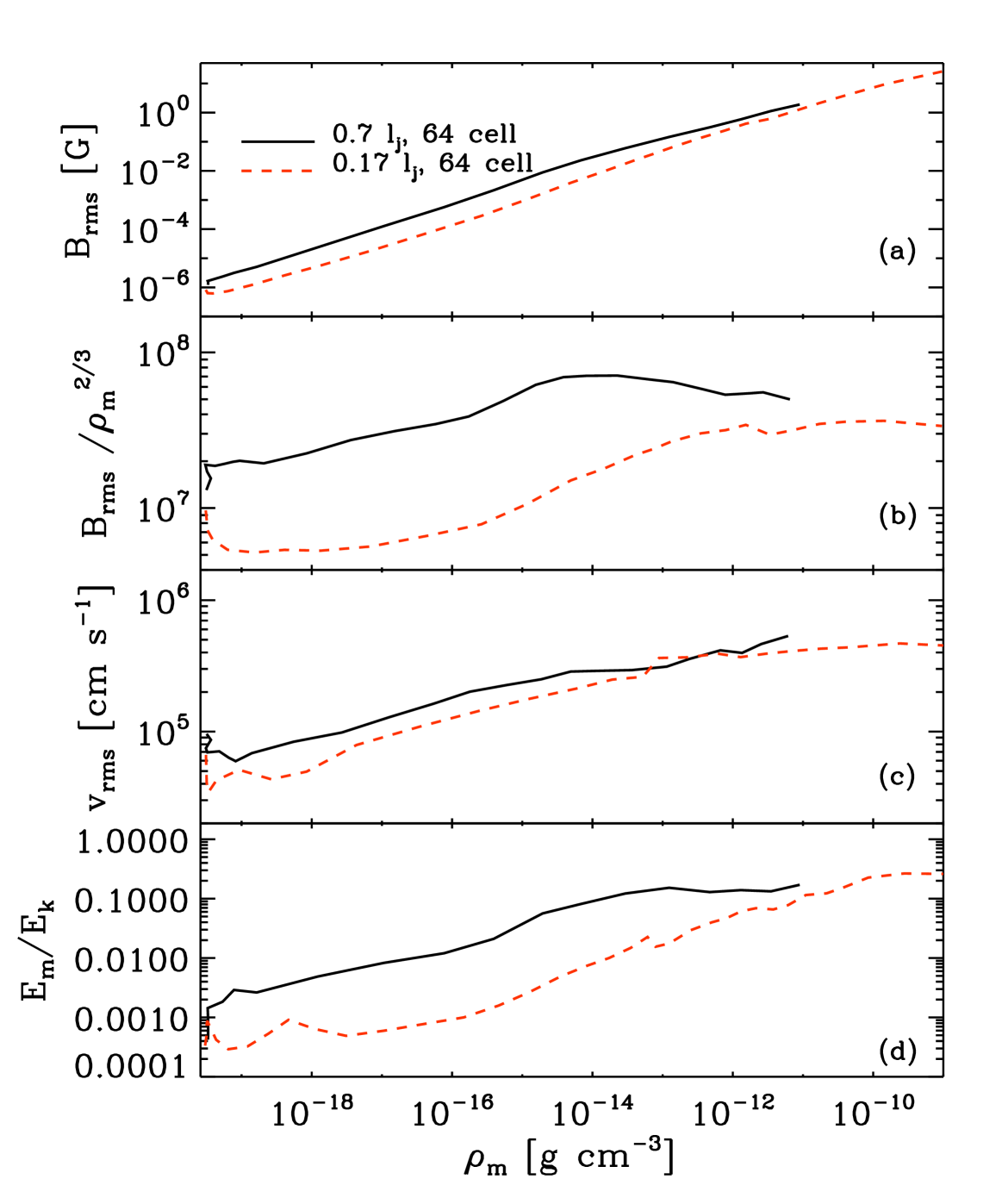
Figure 4: Same as in Fig. 2, but here we compare two runs with zero initial rotation, initial turbulence with $v_{\rm rms}/c_{\rm s}=1.0$ and Jeans resolution of 64 cells for different initial injection scales of turbulence: 0.7 $l_{\rm j}$ (black solid line) and 0.17 $l_{\rm j}$ (red dashed line). When initial turbulence is injected on a smaller scale, the turbulence decays faster leading to an initial decay of $B_{\rm rms}/\rho_{\rm m}^{2/3}$.

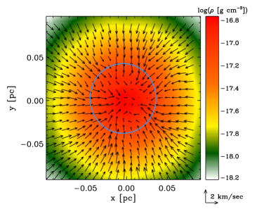
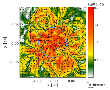
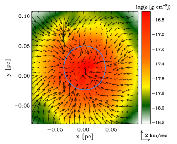
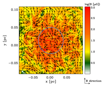
Figure 5: Two-dimensional slices of the density and the total magnetic field for runs with different initial injection scale at a time when the central core density is $\sim 10^{-17}\,\rm{g}\,\,{\rm cm}^{-3}$. The upper row is for $\l_{\rm inj}/\lambda_{\rm J}=0.17$ while the lower row corresponds to $\l_{\rm inj}/\lambda_{\rm J}=0.7$. In the density snapshots, the arrows denote the velocity vectors, while those in the total magnetic field snapshots denote the direction of the local magnetic field. The run with $\l_{\rm inj}/\lambda_{\rm J}=0.17$ shows less turbulent motions inside the Jeans volume compared to the run with $\l_{\rm inj}/\lambda_{\rm J}=0.7$. The magnetic field attains a peak value of $\sim 10^{-4}\,{\rm G}$ for $\l_{\rm inj}/\lambda_{\rm J}=0.17$ and $\sim 10^{-3}\,{\rm G}$ for $\l_{\rm inj}/\lambda_{\rm J}=0.7$ for the same central density of $\rho_{\rm m}\sim 10^{-17}\,\rm{g}\,\,{\rm cm}^{-3}$.

Figure 4 shows the variation of the various physical quantities as a function of the mean density, $\rho_{\rm m}$. With a smaller injection scale, the turbulence decays faster (panel (c) in Fig. 4) compared to the run where $l_{\rm inj}=0.7\,\lambda_{\rm J}$ as more kinetic energy has to be initialised on the smaller scales to get the same overall turbulent Mach number. This can also be seen by comparing the density snapshots in the first column of Fig. 5 where the arrows denote the velocity vectors. These correspond to times when the central core density in both the runs are $\sim 10^{-17}\,\rm{g}\,\,{\rm cm}^{-3}$. The upper plot in this column corresponds to a simulation with $l_{\rm inj}/\lambda_{\rm J}=0.17$ while the plot on the lower panel corresponds to $l_{\rm inj}/\lambda_{\rm J}=0.7$. The run with a smaller injection scale shows less turbulent motions inside the Jeans volume compared to the run where the initial injection scale is peaked on scales of the order $0.7\,\lambda_{\rm J}$.

The second column in Fig. 5 shows that the total magnetic field attains a peak value of $\sim 10^{-4}\,{\rm G}$ for $l_{\rm inj}/\lambda_{\rm J}=0.17$ and about $\sim 10^{-3}\,{\rm G}$ for the run with $l_{\rm inj}/\lambda_{\rm J}=0.7$ at $\rho_{\rm m}=10^{-17}\,\rm{g}\,\,{\rm cm}^{-3}$. The faster decay in the initial turbulence for the smaller injection scale leads to the decay in $B_{\rm rms}/\rho_{\rm m}^{2/3}$ as evident from panel (b) in Fig. 4. Over time, as the turbulence gets regenerated during the collapse, the magnetic field and hence the magnetic energy gets amplified by the dynamo process. The kinematic phase of the dynamo extends to $\rho_{\rm m}\sim 10^{-12}\,\rm{g}\,\,{\rm cm}^{-3}$ for $l_{\rm inj}=0.17\,\lambda_{\rm J}$ with a peak value of $B_{\rm rms}/\rho_{\rm m}^{2/3}\sim 2.5\times 10^{7}$ and up to $\sim 10^{-15}\,\rm{g}\,\,{\rm cm}^{-3}$ for $l_{\rm inj}=0.7\,\lambda_{\rm J}$ with a peak value of $\sim 7\times 10^{7}$. Saturation of the dynamo is once again clearly illustrated by the change in slope of $B_{\rm rms}/\rho_{\rm m}^{2/3}$. For $l_{\rm inj}=0.17\,\lambda_{\rm J}$, this occurs from a density $\sim 10^{-10}\,\rm{g}\,\,{\rm cm}^{-3}$ while for $l_{\rm inj}=0.7\,\lambda_{\rm J}$, saturation starts from $\rho_{\rm m}\sim 10^{-14}\,\rm{g}\,\,{\rm cm}^{-3}$. Comparing this with the evolution of $E_{\rm m}/E_{\rm k}$ in panel (d), we find that the ratio of the energies still continues to increase up to $\rho_{\rm m}\sim 10^{-10}\,\rm{g}\,\,{\rm cm}^{-3}$ for $l_{\rm inj}=0.17\,\lambda_{\rm J}$ and up to $\sim 10^{-13}\,\rm{g}\,\,{\rm cm}^{-3}$ for $l_{\rm inj}=0.7\,\lambda_{\rm J}$. The magnetic energy saturates at about $0.1$ of the equipartition value for this case while for a smaller injection scale, the saturation level is at $\sim 0.3$ of the equipartition value.

3.3 Effect of initial uniform rotation

Finally, we explore the effects of rotation on the collapse and magnetic field amplification. We begin by comparing simulations performed at the same resolution (128 cells per Jeans length) with the initial rotation parameter $\beta$ having values of $0\%$, $4\%$ and $8\%$.

3.3.1 Evolution of the density and the velocity

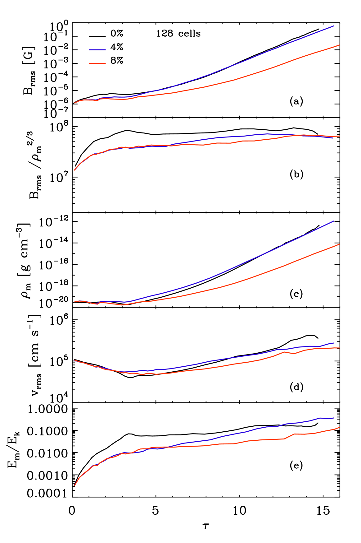
Figure 6: Evolution of the dynamical quantities in the central Jeans volume as a function of $\tau$ for runs with different initial rotation. Panel (a) shows the rms magnetic field strength $B_{\rm rms}$, (b) the evolution of $B_{\rm rms}/\rho_{\rm m}^{2/3}$, showing the turbulent dynamo amplification by dividing out the maximum possible amplification due to perfect flux freezing during spherical collapse, (c) the evolution of the mean density $\rho_{\rm m}$, (d) the rms velocity $v_{\rm rms}$, and (e) the ratio of magnetic to kinetic energy, $E_{\rm m}/E_{\rm k}$. All the simulations correspond to a resolution of 128 cells per Jeans length.

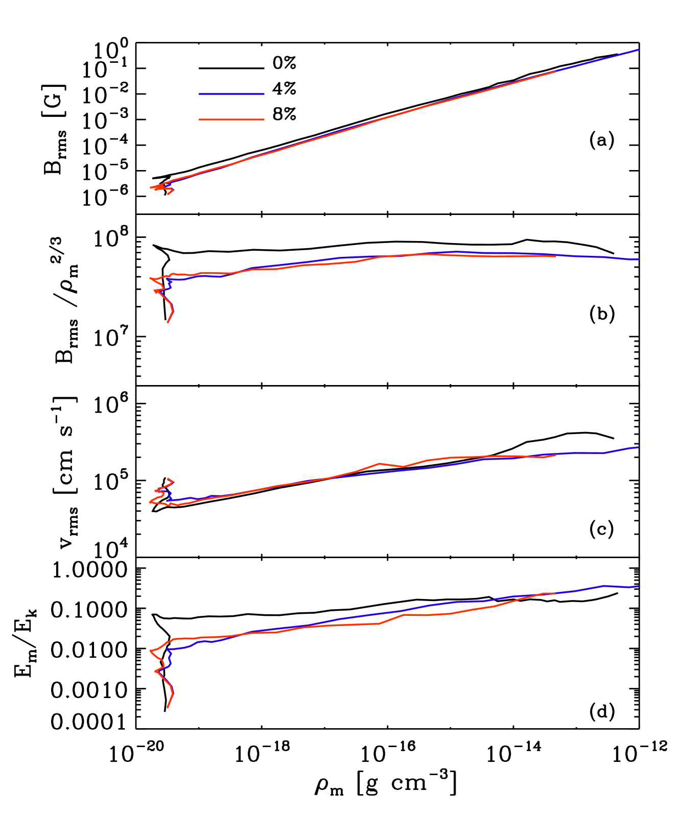
Figure 7: Same as Fig. 6, but now plotted versus the mean density.

In Fig. 6 we show the evolution of various physical quantities as a function of $\tau$ for runs with $\beta=0\%,4\%$ and $8\%$. The same physical quantities are plotted as a function of $\rho_{\rm m}$ in Fig. 7. As reported earlier in Papers I and II, the dynamical evolution of the system shows two distinct phases. First, as the initial turbulent velocity decays, the system exhibits weak oscillatory behavior (up to a time $\tau=4$) with the mean density $\rho_{\rm m}$ evolving similarly for runs with $0\%$, $4\%$ and $8\%$ initial uniform rotation. This is evident from panels (c) and (d) in Figs. 7 and 6 respectively. After this, runaway collapse sets in with peak densities of the order of $\sim 10^{-12}\,\rm{g}\,\,{\rm cm}^{-3}$ being attained for $\beta=0\%$ and $4\%$. Higher value of the initial rotation (e.g. $\beta=8\%$) leads to a delayed collapse as the cloud is more rotationally supported compared to the other two cases (panel (c) in Fig. 6). After the initial decay, the rms velocity increases as the turbulence is regenerated by the collapse.

3.3.2 Magnetic field evolution

Comparing the evolution of the rms magnetic field in the three runs we find from panel (a) in Fig. 7, the magnetic field increases by more than 5 orders of magnitude starting from $1\,\,{\rm\mu G}$ reaching strengths of $0.1\,{\rm G}$ at $\rho_{\rm m}\sim 10^{-13}\,\rm{g}\,\,{\rm cm}^{-3}$. The corresponding evolution with respect to $\tau$ shown in panel (a) of Fig. 6 may seem to suggest that the field amplification is weaker for the $8\%$ run compared to the other two. Panel (b) in both Figs. 6 and 7 shows the evolution of the magnetic field arising due to turbulent motions, i.e, due to small-scale dynamo action. For all the three different runs, the field is exponentially amplified in the initial phase of decaying turbulence (till about $\tau=3-4$). After this, the dynamo continues to amplify the field up to $\tau\sim 13$ or $\rho_{\rm m}\sim 10^{-16}\,\rm{g}\,\,{\rm cm}^{-3}$ but the amplification is no longer exponential. The ratio of the magnetic to kinetic energies (panels e and d in Figs. 6 and 7 also show similar behavior with an initial exponential increase followed by a phase of linear growth.

3.3.3 Dynamo saturation

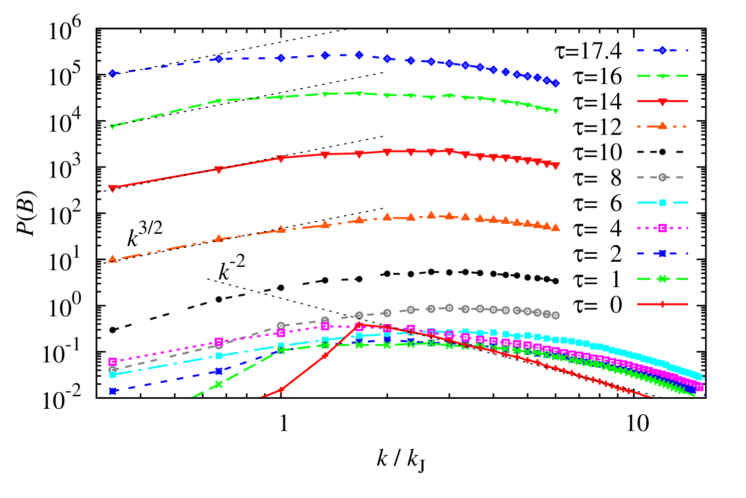
Figure 8: Time evolution of the magnetic field spectra for the run with 128 cells per Jeans length and $E_{\rm rot}/|E_{\rm grav}|=8\%$. The spectra are plotted against the wavenumber normalised to the local Jeans wavenumber. The initial magnetic field spectrum ($\tau=0$) follows a $k^{-2}$ power-law on scales smaller than the peak scale, $k/k_{\rm J}\approx 1.4$ as determined by the initial conditions. After the initial decay of the magnetic energy, the peak of the spectra shifts to $k/k_{\rm J}\approx 3-4$ and stays constant in this range up to $\tau=12$. Because of the smaller eddy turnover times, these high $k/k_{\rm J}$ modes (smaller scales) attain saturation first. The field in the $k/k_{\rm J}<3-4$ modes attain saturation beyond $\tau=12$ with the peak of the spectra now shifted to $k/k_{\rm J}\approx 1$ by the end of the simulation. In addition to the amplification by the dynamo, the magnetic field is also simultaneously amplified by gravitational compression. This leads to an overall rise of the spectrum with time.

Saturation of the dynamo occurs from $\rho_{\rm m}\sim 10^{-15}\,\rm{g}\,\,{\rm cm}^{-3}$ when all the three curves of $B_{\rm rms}/\rho_{\rm m}^{2/3}$ shows a change in slope. From panel (b) in Fig. 7, these curves tend to remain almost constant (red curve) or decay slightly (black and blue curves). However, the $E_{\rm m}/E_{\rm k}$ ratio plotted in panel (d) continues to increase with a weak dependence on the mean density eventually saturating at values of $0.2-0.4$. This once again highlights the fact that $B_{\rm rms}/\rho_{\rm m}^{2/3}$ is a better indicator of dynamo saturation in gravitating systems. A more detailed analysis of dynamo saturation can be obtained from a Fourier analysis of the spectra of the magnetic field. We recall that in Kolmogorov turbulence, the eddy turnover time $t_{\rm ed}=l/v\sim l^{2/3}$. Thus, smaller scale eddies amplify the magnetic field faster due to their shorter eddy turnover times. Therefore, saturation of the magnetic field should first occur on the smaller scales and then gradually be attained on the larger scales. To illustrate this phenomena in a more quantitative fashion, we perform a Fourier analysis of the magnetic field spectra in the collapsing frame of reference for one of our rotation runs with $\beta=8\%$. To compute the spectra, we extract the AMR data in a cube about three times the size of the local Jeans length. For more details on the data extraction procedure and the Fourier analysis we refer the reader to subsection 2.4 of Paper II. Figure 8 shows the time evolution of the magnetic energy spectrum as a function of the wavenumber, $k/k_{\rm J}$, i.e., normalized to the local Jeans wavenumber. Consistent with our initial conditions, the spectrum at $\tau=0$ shows the $P(B)\propto k^{-2}$ power-law scaling. In addition, the initial spectrum is peaked at $k/k_{\rm J}\approx 1.4$ which is in good agreement with our initial conditions where the initial Jeans length of the core is $1.5\,{\rm pc}$ and the peak of magnetic power spectrum is at $0.8\,{\rm pc}$. The time evolution of the magnetic spectrum shows two important features. Firstly, the peak of the initial magnetic spectrum quickly shifts to smaller scales starting from the initial $k/k_{\rm J}=1.4$ and then stays roughly constant at $k/k_{\rm J}\approx 3-4$ till $\tau=12$. This corresponds to about 43 - 32 grid cells which is consistent with the Jeans resolution criterion proposed in Paper II. Next, from $\tau=14$, the peak of the spectrum shifts to smaller $k/k_{\rm J}$ values, i.e., to larger scales. The shift in the peak of the spectrum from $k/k_{\rm J}\approx 3-4$ to $k/k_{\rm J}\approx 1$ at late times implies that the magnetic field at first saturates on the smaller scales followed by saturation on larger scales. Thus, the information obtained from the time evolution of the magnetic field spectra is consistent with theoretical predictions (Subramanian, 1999; Brandenburg & Subramanian, 2005). The magnetic energy however continues to grow with time because the field continues to be amplified by the gravitational collapse.

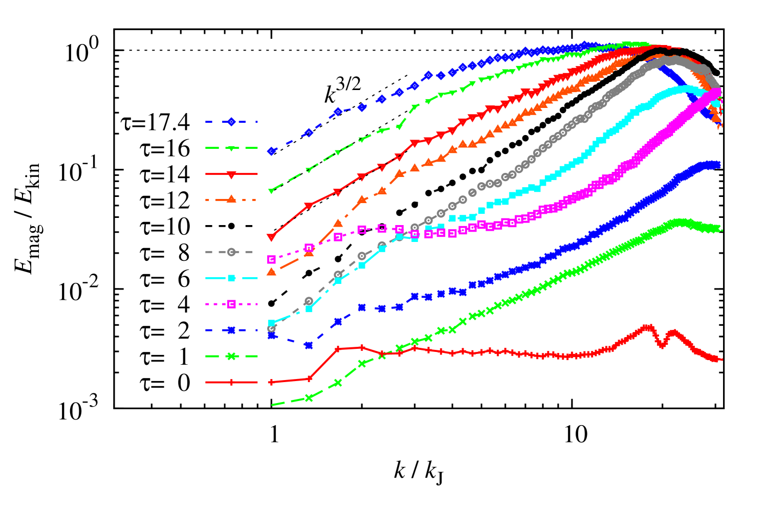
Figure 9: Time evolution of the spectra of the ratio of the magnetic to kinetic energies for the same simulation as in figure 8. As smaller scale eddies amplify the magnetic field faster, the peak of the spectrum initially shifts to smaller scales (i.e., larger $k/k_{\rm J}$ values). By $\tau\sim 10-12$, the magnetic energy attains equipartition with the kinetic energy on scales $k/k_{\rm J}\sim 20$. Further time evolution shows that the peak now spreads to larger scales (i.e., smaller $k/k_{\rm J}$ values) with the field attaining equipartition on scales $k/k_{\rm J}=7-10$ at $\tau=17.4$. This plot therefore illustrates the saturation mechanism of the dynamo in a self-gravitating system.

To further analyse the level of saturation we plot the time evolution spectra of the ratio of the magnetic to kinetic energies in Fig. 9. Since we extract about three times the volume for our Fourier analysis, we have taken a mean density of $\rho_{\rm m}\sim 10^{-21}\,\rm{g}\,\,{\rm cm}^{-3}$ resulting in an initial value of $E_{\rm m}/E_{\rm k}\sim 2\times 10^{-3}$. We also remove all large-scale velocity contributions (i.e., global rotation and infall) from the kinetic energy. Since the smaller scale eddies amplify the field faster, $E_{\rm m}/E_{\rm k}$ first starts to peak at large $k/k_{\rm J}$ for $\tau>0$. At $\tau=12$, the magnetic energy attains equipartition with the kinetic energy on a scale $k/k_{\rm J}=20$. Once saturation has been attained on this scale, the peak of the spectrum now starts to shift to smaller $k/k_{\rm J}$. By $\tau=17.4$, the peak of the spectrum occurs at $k/k_{\rm J}=7-10$, i.e., saturation of the dynamo is now achieved on larger scales. This gradual shift of the peak of $E_{\rm m}/E_{\rm k}\sim 1$ to smaller $k/k_{\rm J}$ demonstrates the saturation of the dynamo and a possible development of a large-scale coherent magnetic field if the simulation is evolved further in time. The spectra further show that the magnetic field becomes dynamically important to back react on the flow on scales $k/k_{\rm J}=20$ by $\tau=12$ with the magnetic energy attaining equipartition with the kinetic energy. By the end of the simulation, equipartition is achieved on even larger scales.

3.3.4 Radial profiles

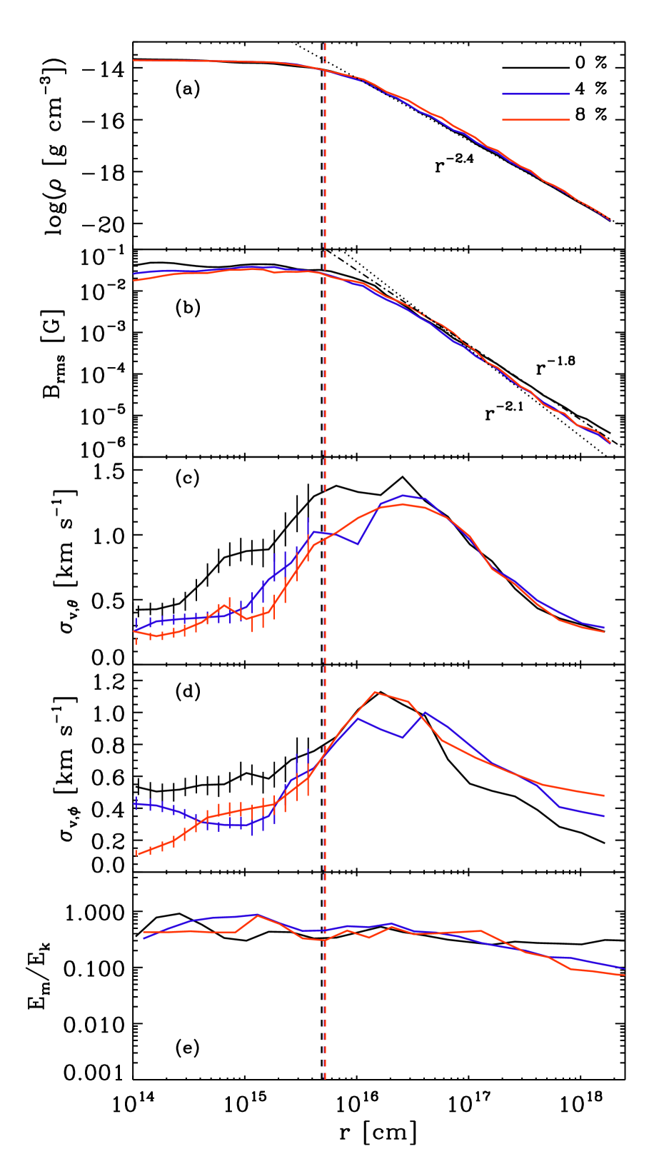
Figure 10: Radial profiles of the density in panel (a), the rms magnetic field in panel (b), components of the velocity dispersion, $\sigma_{\rm v,\theta}$ and $\sigma_{\rm v,\phi}$ in panels (c) and (d) respectively and the ratio of magnetic to kinetic energies in panel (e) at a time when runs with different initial rotation reached the same core density as shown in panel (a). Dashed vertical lines depict the local Jeans radius. Error bars are shown as solid vertical lines (panels c and d) inside the Jeans radius. The data are obtained from simulations with $\lambda_{\rm J}$ resolved by 128 cells.

Figure 10 shows the radial profile of the density, the rms magnetic field, the polar and azimuthal velocity dispersions, $\sigma_{\rm v,\theta}$ , $\sigma_{\rm v,\phi}$ and the ratio of magnetic to kinetic energies ($E_{\rm m}/E_{\rm k}$) for runs with $\beta=0,4$ and $8\%$ initial rotation at a time when all the three attain the same core density. Similar to earlier results in Papers I and II, the density develops a flat inner core and falls off as $r^{-2.4}$ due to the effective equation of state with $\Gamma=1.1$ (see Larson, 1969). Panel (b) shows that the rms magnetic field attains peak values between $0.02-0.04\,{\rm G}$ within the Jeans volume. The radial profile of $B_{\rm rms}$ shows a radial dependence $\propto(r^{-1.8}-r^{-2.1})$ for the three runs. This is significantly steeper than the expectation from pure flux freezing where $B(r)\propto r^{-4/3}$. The velocity dispersion shown in panels (c) and (d) increases in the envelope and drops inside the Jeans volume. This is most likely due to the back reaction of the strong magnetic fields generated inside the Jeans volume. The ratio of the magnetic to kinetic energies plotted in panel (e) attains values in the range $\sim 0.3-0.8$ inside the Jeans volume.

3.3.5 Morphological features

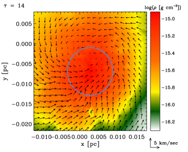
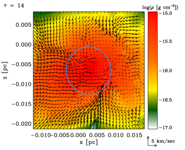
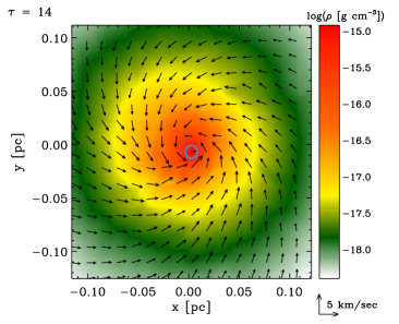
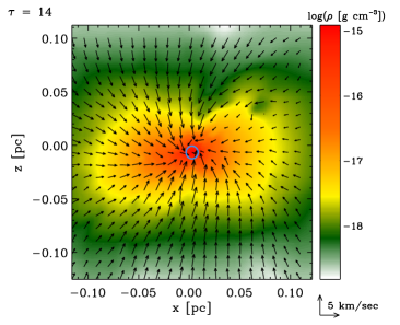
Figure 11: Morphology of the cloud: Two-dimensional slices of the density for a run with $8\%$ initial uniform rotation through the center of the collapsing core at $\tau=14$. The top row corresponds to zoomed-in slices in the $x$-$y$ plane and $x$-$z$ plane, while the bottom row corresponds to zoomed-out slices in the $x$-$y$ plane and in the $x$-$z$ plane. The arrows denote the velocity field vectors, while the circle denotes the local Jeans volume. The zoomed out $x$-$z$ slice on the bottom row shows the gradual flattening of the collapsed BE sphere due to the initial rotation.

What effect does rotation have on the morphology of the cloud and does it lead to any change in the morphology of the small-scale dynamo generated field? In Fig. 11 we show two-dimensional snapshots of the density field in two planes: $x-y$ and $x-z$ for the run with $\beta=8\%$ at a time when the central core density is $\sim 10^{-15}\,\rm{g}\,\,{\rm cm}^{-3}$. The upper panel shows the zoomed-in slices, while the lower panel shows the zoomed-out version of the density field. Turbulent motions are dominant inside the Jeans volume as can be seen from the plotted velocity vectors in the zoomed-in slice in the $x-z$ plane. Rotational motion of the gas cloud is clearly seen from the $x-y$ slice in the lower panel. In conformity with known results, uniform rotation leads to a flattening of the gas cloud shown in the $x-z$ slice illustration in the lower panel.

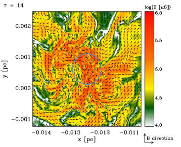
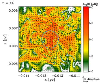
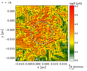
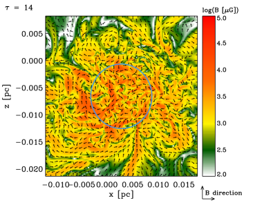
Figure 12: Magnetic field structures: Two-dimensional slices of the total magnetic field through the center of the collapsing sore at $\tau=14$. The upper row shows the $x$-$y$ and the $x$-$z$ plane snapshots for a run with no initial uniform rotation. The lower row shows the $x$-$y$ and the $x$-$z$ plane snapshots for a run with $8\%$ uniform rotation. As before, the circles depict the local Jeans volume. The arrows denote the direction of the local magnetic field.

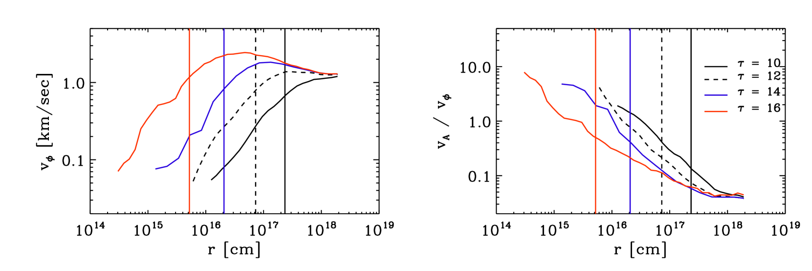
Figure 13: Radial profiles of the toroidal velocity $v_{\phi}$ (left panel) and the Alfv́en velocity $v_{\rm A}$ normalised to $v_{\phi}$ (right panel) at different times for a run with $8\%$ initial rotation. The vertical lines indicate the local Jeans radius at different times. Runs plotted here are from simulations where $\lambda_{\rm J}$ is resolved with 128 cells.

Quite interestingly, the morphology of the magnetic field in the saturated state does not seem to depend significantly on the amount of initial rotation (see Fig. 12). The magnetic field is randomly oriented within the local Jeans volume. This is reminiscent of the typical magnetic field structures seen in simulations of small-scale dynamo action where turbulence is driven artificially with random forcing (Brandenburg & Subramanian, 2005; Federrath et al., 2011a). In our case, the turbulence is driven completely by the gravitational collapse (Klessen & Hennebelle, 2010, Papers I and II). In Fig. 12 we plot the slices of the total magnetic field in $x-y$ and $x-z$ planes for two different cases: the first row corresponds to no net rotation and the second row corresponds to $8\%$ initial rotation. In both cases, the magnetic field is randomly oriented, attaining peak values of $0.1\,\,{\rm\mu G}$ within the central Jeans volume. In Fig. 13, we show the radial profiles of the toroidal velocity $v_{\phi}$ (left panel) and the ratio of the Alfv́en velocity normalized to the toroidal velocity (right panel) at different times. The toroidal velocity increases initially as we move from the outer to inner radii and then drops inside the local Jeans radius. This is because, inside the Jeans volume, a protostellar core of uniform density (see panel (a) in Fig. 10 where the density forms a flat inner core inside the Jeans radius) has formed which rotates like a solid body. The reason why uniform rotation does not introduce any morphological change in the magnetic field can be explained with the help of the radial profile of the ratio of the Alfv́en to the rotational velocity shown in the above figure. At any given time, the increase in the ratio $v_{\rm A}/v_{\phi}$ as one proceeds from the outer to inner regions implies that the magnetic field is amplified on a much shorter timescale than the orbital time of the cloud. The dynamical effect of rotation on the magnetic field morphology will become observable at much later times, when the orbital timescale and the timescale on which the magnetic field is amplified become comparable.

3.3.6 Resolution effects

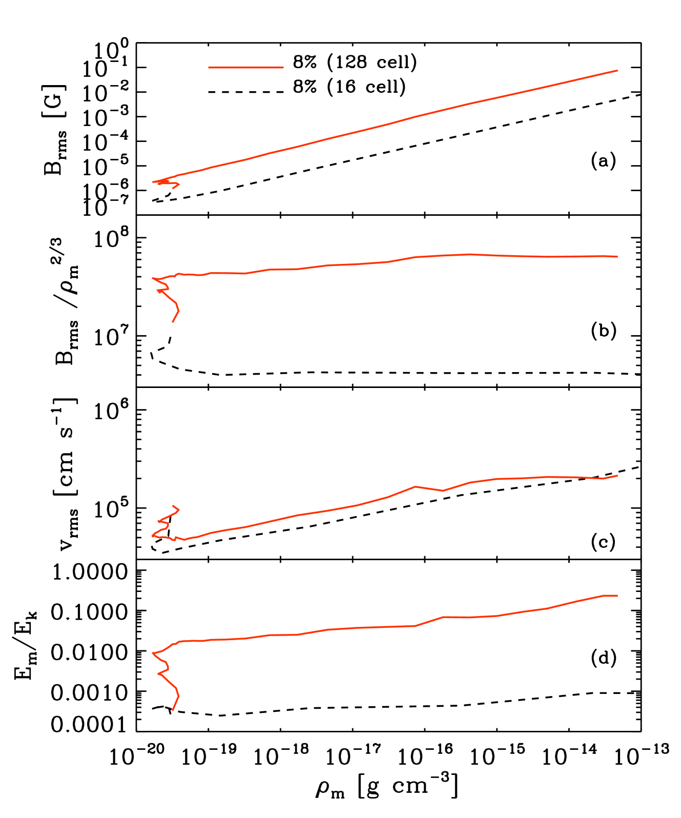
Figure 14: Comparison between two runs with initial rotation of $E_{\rm rot}/|E_{\rm grav}|=8\%$, where the Jeans length was resolved by 128 cells (solid line) and 16 cells (dashed line), respectively. In comparison to our highest resolution simulation (128 cells), this leads to an order of magnitude difference in the magnetic field amplification. No dynamo amplification occurs in the 16 cell run as is evident from panel b (see also Papers I and II for a more detailed study of the resolution effects).

To make a direct comparison of how the collapse and field amplification are affected by rotation, we compare two simulations with the same value of the $\beta$ parameter, but at two different resolutions, one at $16$ cells and the other at a resolution of $128$ cells. The utility of this approach lies in the fact that when the local Jeans length is resolved by only $16$ cells, the small-scale dynamo is not excited (as turbulent motions are under-resolved) and the magnetic field is only amplified by gravitational compression in a rotating gas cloud. The comparison is shown in Fig. 14, between a 16 cell and a 128 cell run both having $\beta=8\%$ initial uniform rotation. For the 16 cells run, the field amplification arises purely due gravitational compression of the field lines. This leads to an order of magnitude difference in the evolution of the rms magnetic field (panel (a) in Fig. 14 ). However, as explained earlier, the growth rate of the small-scale dynamo depends on the resolution. Thus, an order of magnitude difference in this case should be taken as a lower limit. The plot in panel (b) confirms the absence of any small-scale dynamo for the 16 cell run as the $B_{\rm rms}/\rho_{\rm m}^{2/3}$ curve at first decays and then stays roughly constant while for the 128 cell run, there is an initial increase in $B_{\rm rms}/\rho_{\rm m}^{2/3}$ followed by saturation at a value $B_{\rm rms}/\rho_{\rm m}^{2/3}\sim 6\times 10^{7}$. Also, from panel (d), we find that while the ratio of $E_{\rm m}/E_{\rm k}$ increases rapidly to values $\sim 10^{-2}$ for the 128 cell run, there is no corresponding increase for the 16 cell run. We refer the reader to Papers I and II for a more detailed analysis of resolution effects.

4 Summary and Conclusions

In this paper, we have presented a detailed study of the influence of initial conditions on the gravitational collapse and magnetic field amplification of a dense gas cloud. We chose initial and environmental conditions that are reminiscent of the conditions in primordial mini-halos that lead to the formation of the first stars in the Universe. We purposely chose the initial strength of the magnetic field to be $\sim 1\,\,{\rm\mu G}$ with an $E_{\rm m}/E_{\rm k}\sim 10^{-4}$ to capture the saturation of the small-scale dynamo. In this respect, this study goes beyond our earlier studies (Papers I and II) where we only considered the kinematic regime of the dynamo growth. Since dynamo amplification of the magnetic field occurs due to turbulent fluid motions, we varied the strength and injection scale of the initial turbulence in this study. In addition, we have also studied the influence of initial uniform rotation on the collapse and magnetic field amplification. The general behavior of the magnetic field amplification presented here reveals two distinct phases: first, the total magnetic field is amplified by both the gravitational compression and the small-scale dynamo. Later, the small-scale dynamo saturates after which the field amplification is driven only by compression. Our main results obtained from the systematic study are summarised as follows:

• We started by exploring the effect of varying the initial strength of the turbulent velocity. The parameter range we explored concerns an initial $v_{\rm rms}/c_{\rm s}=0.2,0.4,1.0,2.0$ and $4.0$. The total magnetic field in these simulations is amplified by more than 6 orders of magnitude, reaching peak values of $\sim 1\,{\rm G}$ at densities of $\sim 10^{-12}\,\rm{g}\,\,{\rm cm}^{-3}$. Initially, the small-scale dynamo provides additional field amplification to the regular amplification occurring due to gravitational compression. Later, we find that the small-scale dynamo saturates. In almost all the cases, except when the initial $v_{\rm rms}=4\,c_{\rm s}$, the amplification of the magnetic field by the small-scale dynamo continues till $\sim\tau=10$. This corresponds to the kinematic phase of the dynamo. In this phase, $B_{\rm rms}/\rho_{\rm m}^{2/3}$ attains a peak value in the range $\sim(2-6)\times 10^{7}$ (with respect to the initial value) in the density range $\rho_{\rm m}\sim(10^{-13}-10^{-10})\,\rm{g}\,\,{\rm cm}^{-3}$. The growth rate of $B_{\rm rms}/\rho_{\rm m}^{2/3}$ at first increases with the increase in initial subsonic Mach numbers and then decreases in the supersonic regime. Federrath et al. (2011a), also report a similar behavior with Mach number in forced turbulence-in-a-box simulations of small-scale dynamo action. Beyond $\rho_{\rm m}\sim 10^{-14}\,\rm{g}\,\,{\rm cm}^{-3}$, $B_{\rm rms}/\rho_{\rm m}^{2/3}$ shows a distinct change in slope indicating that the dynamo reaches saturation. The total field amplification in the saturated phase is now only due to gravitational compression. The magnetic energy still shows a mild increase reaching values of $0.2-0.4$ of the equipartition strength for the parameter range we explore. Thus, $B_{\rm rms}/\rho_{\rm m}^{2/3}$ is a more suitable indicator of dynamo saturation in self-gravitating systems.
  

• Next, we explored the effect of varying the initial injection scale of turbulence. We compared two simulations with $l_{\rm inj}=0.17\,\lambda_{\rm J}$ and $0.7\,\lambda_{\rm J}$. With a smaller injection scale, the turbulence decays faster as more kinetic energy has to be initialized on the smaller scales to get the same overall turbulent Mach number. The smaller scales are therefore dissipated more quickly resulting in the early collapse by $\tau\sim 1$ compared to the other run where runaway collapse sets in at $\tau\sim 4$. The kinematic phase of the dynamo extends to $\rho_{\rm m}\sim 10^{-12}\,\rm{g}\,\,{\rm cm}^{-3}$ for $l_{\rm inj}=0.17\,\lambda_{\rm J}$ and up to $\sim 10^{-15}\,\rm{g}\,\,{\rm cm}^{-3}$ for $l_{\rm inj}=0.7\,\lambda_{\rm J}$. Saturation of the dynamo is once again clearly illustrated by the change in slope of $B_{\rm rms}/\rho_{\rm m}^{2/3}$ compared to the evolution of $E_{\rm m}/E_{\rm k}$. For $l_{\rm inj}=0.17\,\lambda_{\rm J}$, this occurs from a density $\sim 10^{-10}\,\rm{g}\,\,{\rm cm}^{-3}$ while for $l_{\rm inj}=0.7\,\lambda_{\rm J}$, saturation starts from $\rho_{\rm m}\sim 10^{-14}\,\rm{g}\,\,{\rm cm}^{-3}$. By the end of the simulation, the magnetic energy attains values in the range $0.1-0.3$ of the equipartition values for these two runs.
  

• Finally, we explored the effect of uniform initial rotation. We considered three simulations where the rotation parameter $\beta$ has values of $0\%,4\%$ and $8\%$. The dynamical evolution of the system shows two distinct phases: an initial turbulent decay phase followed by a runaway collapse phase where the turbulence gets regenerated by the gravitational collapse. The dynamo generated magnetic field $B_{\rm rms}/\rho_{\rm m}^{2/3}$ saturates for all the three runs when the central core density $\rho_{\rm m}\sim 10^{-15}\,\rm{g}\,\,{\rm cm}^{-3}$. The saturation behavior is clearly revealed in the time evolution of magnetic field spectra (Fig. 8) where the peak of the spectrum gradually shifts to larger scales (i.e., smaller $k/k_{\rm J}$ values) at late times. Consistent with earlier theoretical predictions, magnetic energy attains equipartition with the kinetic energy first on smaller scales and then gradually on larger scales. This is shown in Fig. 9. Our resolution study further shows that the dynamo amplification leads to an order of magnitude difference in the magnetic field amplification. Since the dynamo amplification is resolution dependent (higher resolution leads to stronger field amplification), this difference should be taken as a lower bound.

In summary, using idealized simulations, our systematic study has probed for the first time, the effect of different initial conditions on the dynamo amplification of the magnetic field and its saturation for the specific case of primordial cloud collapse. Our choice of the initial field strength allowed us to probe both the kinematic and the saturation regime of the small-scale dynamo. Detailed analysis of the magnetic field spectra shows that saturation is achieved initially on smaller scales and then later on, the magnetic field saturates on larger scales. In all our simulations presented here, the magnetic energy continues to grow at the expense of the kinetic energy eventually attaining values in the range, $E_{\rm m}/E_{\rm k}\sim 0.1-0.4$. This range of values are roughly in agreement with previous analytical (Subramanian, 1999) and numerical work on small-scale dynamo action in forced turbulence (Haugen et al., 2004; Brandenburg & Subramanian, 2005; Federrath et al., 2011a). For the case of a primordial cloud collapse which we explore here, the small-scale dynamo comes across as an efficient process to generate strong seed fields on scales comparable to the scale of turbulence (in our case, the local Jeans length). These strong seed fields could potentially lead to the generation of large-scale coherent magnetic fields on scales much larger than the scale of turbulence (in our case on scales $k/k_{\rm J}\ll 1$) via large-scale dynamo mechanisms (Ruzmaikin et al., 1988; Hanasz et al., 2009; Jedamzik & Sigl, 2011). The implications of such coherent magnetic fields has been previously explored in the works of Pudritz & Silk (1989) and Tan & Blackman (2004). Starting from seed magnetic fields such as the ones generated by a small-scale dynamo, Tan & Blackman (2004) show that coherent magnetic fields can be produced in situ in primordial star forming disks.

Numerical simulations with an initially coherent magnetic field have previously shown the formation of jets and bipolar outflows (e.g., Banerjee & Pudritz, 2006; Machida et al., 2006; Banerjee & Pudritz, 2007; Machida et al., 2008). Recent work by Pietarila Graham et al. (2010) find evidence of small-scale dynamo action in the solar surface. Silk & Langer (2006) infer that magnetic fields can be amplified by the magneto-rotational instability (MRI) in the disk leading to coherent magnetic fields. The presence of a small-scale dynamo can potentially further amplify the seed fields in the disk. It remains to be seen what effect, if such large-scale magnetic fields generated during the primordial collapse, have for example - on the formation process of the first stars. Recent hydrodynamical calculations of first star formation (Greif et al., 2011; Clark et al., 2011) have shown that the disks that formed around the first young stars were unstable to gravitational fragmentation, possibly leading to the formation of small binary and higher-order systems. Whether or not, magnetic fields generated and amplified by dynamo processes can influence this scenario is an open question. Magnetic fields may also have a bearing on the rotation speed of the first stars (Stacy et al., 2011). Moreover, magnetic fields generated by dynamo processes in the primordial universe and ejected in outflows will have implications for the formation of the second generation of stars and the first galaxies. More detailed investigations including other relevant physics and additional processes like primordial chemistry and cooling, non-ideal MHD and radiative feedback effects are needed in the near future to address these possibilities.

References

- Abel et al. (2002) Abel, T., Bryan, G. L., & Norman, M. L. 2002, Science, 295, 93
- Banerjee & Pudritz (2006) Banerjee, R., & Pudritz, R. E. 2006, ApJ, 641, 949
- Banerjee & Pudritz (2007) —. 2007, ApJ, 660, 479
- Beck (2004) Beck, R. 2004, Astrophysics & Space Science, 289, 293
- Beck & Hoernes (1996) Beck, R., & Hoernes, P. 1996, Nature, 379, 47
- Beck et al. (1994) Beck, R., Poezd, A. D., Shukurov, A., & Sokoloff, D. D. 1994, A&A, 289, 94
- Bernet et al. (2008) Bernet, M. L., Miniati, F., Lilly, S. J., Kronberg, P. P., & Dessauges-Zavadsky, M. 2008, Nature, 454, 302
- Boldyrev & Cattaneo (2004) Boldyrev, S., & Cattaneo, F. 2004, Physical Review Letters, 92, 144501
- Bonnor (1956) Bonnor, W. B. 1956, MNRAS, 116, 351
- Bouchut et al. (2007) Bouchut, F., Klingenberg, C., & Waagan, K. 2007, Numerische Mathematik, 108, 7
- Bouchut et al. (2010) —. 2010, Numerische Mathematik, 115, 647
- Brandenburg & Subramanian (2005) Brandenburg, A., & Subramanian, K. 2005, Phys. Rep., 417, 1
- Bryan & Norman (1998) Bryan, G. L., & Norman, M. L. 1998, ApJ, 495, 80
- Carilli & Taylor (2002) Carilli, C. L., & Taylor, G. B. 2002, Ann. Rev. Astron. Astrophys., 40, 319
- Clark et al. (2011) Clark, P. C., Glover, S. C. O., Smith, R. J., Greif, T. H., Klessen, R. S., & Bromm, V. 2011, Science, 331, 1040
- Dolag et al. (1999) Dolag, K., Bartelmann, M., & Lesch, H. 1999, A&A, 348, 351
- Duffin & Pudritz (2009) Duffin, D. F., & Pudritz, R. E. 2009, ApJ, 706, L46
- Ebert (1955) Ebert, R. 1955, Zeitschrift fur Astrophysik, 37, 217
- Federrath et al. (2011a) Federrath, C., Chabrier, G., Schober, J., Banerjee, R., Klessen, R. S., & Schleicher, D. R. G. 2011a, Physical Review Letters, 107, 114504
- Federrath et al. (2011b) Federrath, C., Sur, S., Schleicher, D. R. G., Banerjee, R., & Klessen, R. S. 2011b, ApJ, 731, 62
- Fryxell et al. (2000) Fryxell, B., Olson, K., Ricker, P., Timmes, F. X., Zingale, M., Lamb, D. Q., MacNeice, P., Rosner, R., Truran, J. W., & Tufo, H. 2000, ApJS, 131, 273
- Govoni & Feretti (2004) Govoni, F., & Feretti, L. 2004, International Journal of Modern Physics D, 13, 1549
- Grasso & Rubinstein (2001) Grasso, D., & Rubinstein, H. R. 2001, Phys. Rep., 348, 163
- Greif et al. (2011) Greif, T., Springel, V., White, S., Glover, S., Clark, P., Smith, R., Klessen, R., & Bromm, V. 2011, ArXiv e-prints
- Greif et al. (2008) Greif, T. H., Johnson, J. L., Klessen, R. S., & Bromm, V. 2008, MNRAS, 387, 1021
- Hanasz et al. (2009) Hanasz, M., Wóltański, D., & Kowalik, K. 2009, ApJL, 706, L155
- Haugen et al. (2004) Haugen, N. E., Brandenburg, A., & Dobler, W. 2004, Phys. Rev. E, 70, 016308
- Hennebelle & Teyssier (2008) Hennebelle, P., & Teyssier, R. 2008, A&A, 477, 25
- Jedamzik & Sigl (2011) Jedamzik, K., & Sigl, G. 2011, Phys. Rev. D, 83, 103005
- Kazantsev (1968) Kazantsev, A. P. 1968, Soviet Journal of Experimental and Theoretical Physics, 26, 1031
- Klessen & Hennebelle (2010) Klessen, R. S., & Hennebelle, P. 2010, A&A, 520, A17+
- Kulsrud et al. (1997) Kulsrud, R. M., Cen, R., Ostriker, J. P., & Ryu, D. 1997, ApJ, 480, 481
- Larson (1969) Larson, R. B. 1969, MNRAS, 145, 271
- Machida et al. (2008) Machida, M. N., Inutsuka, S.-i., & Matsumoto, T. 2008, ApJ, 676, 1088
- Machida et al. (2006) Machida, M. N., Omukai, K., Matsumoto, T., & Inutsuka, S. 2006, ApJ, 647, L1
- Maki & Susa (2004) Maki, H., & Susa, H. 2004, ApJ, 609, 467
- Maki & Susa (2007) —. 2007, PASJ, 59, 787
- Miniati et al. (2001) Miniati, F., Jones, T. W., Kang, H., & Ryu, D. 2001, ApJ, 562, 233
- Neronov & Vovk (2010) Neronov, A., & Vovk, I. 2010, Science, 328, 73
- Omukai et al. (2005) Omukai, K., Tsuribe, T., Schneider, R., & Ferrara, A. 2005, ApJ, 626, 627
- O’Shea & Norman (2007) O’Shea, B. W., & Norman, M. L. 2007, ApJ, 654, 66
- Pietarila Graham et al. (2010) Pietarila Graham, J., Cameron, R., & Schüssler, M. 2010, ApJ, 714, 1606
- Pinto & Galli (2008) Pinto, C., & Galli, D. 2008, A&A, 484, 17
- Pudritz & Silk (1989) Pudritz, R. E., & Silk, J. 1989, ApJ, 342, 650
- Ricker & Sarazin (2001) Ricker, P. M., & Sarazin, C. L. 2001, ApJ, 561, 621
- Ruzmaikin et al. (1988) Ruzmaikin, A. A., Sokolov, D. D., & Shukurov, A. M., eds. 1988, Astrophysics and Space Science Library, Vol. 133, Magnetic fields of galaxies
- Ryu et al. (2008) Ryu, D., Kang, H., Cho, J., & Das, S. 2008, Science, 320, 909
- Schekochihin et al. (2002) Schekochihin, A. A., Boldyrev, S. A., & Kulsrud, R. M. 2002, ApJ, 567, 828
- Schekochihin et al. (2004) Schekochihin, A. A., Cowley, S. C., Taylor, S. F., Maron, J. L., & McWilliams, J. C. 2004, ApJ, 612, 276
- Schindler & Mueller (1993) Schindler, S., & Mueller, E. 1993, Astron. Astrophys., 272, 137
- Schleicher et al. (2010) Schleicher, D. R. G., Banerjee, R., Sur, S., Arshakian, T. G., Klessen, R. S., Beck, R., & Spaans, M. 2010, A&A, 522, A115+
- Schober et al. (2011) Schober, J., Schleicher, D., Federrath, C., Klessen, R., & Banerjee, R. 2011, ArXiv e-prints
- Silk & Langer (2006) Silk, J., & Langer, M. 2006, MNRAS, 371, 444
- Stacy et al. (2011) Stacy, A., Bromm, V., & Loeb, A. 2011, MNRAS, 413, 543
- Subramanian (1999) Subramanian, K. 1999, Phys. Rev. Lett., 83, 2957
- Subramanian et al. (2006) Subramanian, K., Shukurov, A., & Haugen, N. E. L. 2006, MNRAS, 366, 1437
- Sur et al. (2010) Sur, S., Schleicher, D. R. G., Banerjee, R., Federrath, C., & Klessen, R. S. 2010, ApJ, 721, L134
- Tan & Blackman (2004) Tan, J. C., & Blackman, E. G. 2004, ApJ, 603, 401
- Tavecchio et al. (2010) Tavecchio, F., Ghisellini, G., Foschini, L., Bonnoli, G., Ghirlanda, G., & Coppi, P. 2010, MNRAS, 406, L70
- Turk et al. (2009) Turk, M. J., Abel, T., & O’Shea, B. 2009, Science, 325, 601
- Turk et al. (2011) Turk, M. J., Oishi, J. S., Abel, T., & Bryan, G. 2011, ArXiv e-prints
- Vainshtein (1982) Vainshtein, S. I. 1982, Zhurnal Eksperimental noi i Teoreticheskoi Fiziki, 83, 161
- Waagan (2009) Waagan, K. 2009, Journal of Computational Physics, 228, 8609
- Waagan et al. (2011) Waagan, K., Federrath, C., & Klingenberg, C. 2011, Journal of Computational Physics, 230, 3331
- Wise & Abel (2007) Wise, J. H., & Abel, T. 2007, ApJ, 665, 899
- Wise et al. (2008) Wise, J. H., Turk, M. J., & Abel, T. 2008, ApJ, 682, 745
- Xu et al. (2009) Xu, H., Li, H., Collins, D. C., Li, S., & Norman, M. L. 2009, ApJ, 698, L14
- Xu et al. (2011) —. 2011, ArXiv e-prints
- Yoshida et al. (2008) Yoshida, N., Omukai, K., & Hernquist, L. 2008, Science, 321, 669