Greedy Sequential Maximal Independent Set and Matching
are Parallel on Average

The greedy sequential algorithm for maximal independent set (MIS) loops over the vertices in arbitrary order adding a vertex to the resulting set if and only if no previous neighboring vertex has been added. In this loop, as in many sequential loops, each iterate will only depend on a subset of the previous iterates (i.e. knowing that any one of a vertex’s neighbors is in the MIS, or knowing that it has no previous neighbors, is sufficient to decide its fate one way or the other). This leads to a dependence structure among the iterates. If this structure is shallow then running the iterates in parallel while respecting the dependencies can lead to an efficient parallel implementation mimicking the sequential algorithm.

In this paper, we show that for any graph, and for a random ordering of the vertices, the dependence length of the sequential greedy MIS algorithm is polylogarithmic ($O(\log^{2}n)$ with high probability). Our results extend previous results that show polylogarithmic bounds only for random graphs. We show similar results for a greedy maximal matching (MM). For both problems we describe simple linear work parallel algorithms based on the approach. The algorithms allow for a smooth tradeoff between more parallelism and reduced work, but always return the same result as the sequential greedy algorithms. We present experimental results that demonstrate efficiency and the tradeoff between work and parallelism.

Keywords: Parallel algorithms, maximal independent set, maximal matching

1 Introduction

The maximal independent set (MIS) problem is given an undirected graph $G=(V,E)$ to return a subset $U\subseteq V$ such that no vertices in $U$ are neighbors of each other (independent set), and all vertices in $V\setminus U$ have a neighbor in $U$ (maximal). The MIS is a fundamental problem in parallel algorithms with many applications [17]. For example if the vertices represent tasks and each edge represents the constraint that two tasks cannot run in parallel, the MIS finds a maximal set of tasks to run in parallel. Parallel algorithms for the problem have been well studied [16, 17, 1, 12, 9, 11, 10, 7, 4]. Luby’s randomized algorithm [17], for example, runs in $O(\log|V|)$ time on $O(|E|)$ processors of an CRCW PRAM and can be converted to run in linear work. The problem, however, is that on a modest number of processors it is very hard for these parallel algorithms to outperform the very simple and fast sequential greedy algorithm. Furthemore the parallel algorithms give different results than the sequential algorithm. This can be undesirable in a context where one wants to choose between the algorithms based on platform but wants deterministic answers.

In this paper we show that, perhaps surprisingly, a trivial parallelization of the sequential greedy algorithm is in fact highly parallel (polylogarithmic time) when the order of vertices is randomized. In particular simply by processing each vertex as in the sequential algorithm but as soon as it has no earlier neighbors gives a parallel linear work algorithm. The MIS returned by the sequential greedy algorithm, and hence also its parallelization, is referred to as the lexicographically first MIS [6]. In a general undirected graph and an arbitrary order, the problem of finding a lexicographically first MIS is P-complete [6, 13], meaning that it is unlikely that any efficient low-depth parallel algorithm exists for this problem. Moreover, it is even P-complete to approximate the size of the lexicographically first MIS [13]. Our results show that for any graph and for the vast majority of orders the lexicographically first MIS has polylogarithmic depth.

Beyond theoretical interest the result has important practical implications. Firstly it allows for a very simple and efficient parallel implementation of MIS that can trade off work with depth. The approach is instead of processing all vertices in parallel to process prefixes of the vertex ordering in parallel. Using smaller prefixes reduces parallelism but also reduces redundant work. The limit of a prefix of size one gives the sequential algorithm with no redundant work. We show bounds on prefix size that guarantee linear work. The second implication is that once an ordering is fixed, the approach guarantees the same result whether run in parallel or sequentially or, in fact, choosing any schedule of the iterations that respects the dependences. Such determinism can be an important property of parallel algorithms [3, 2].

Our results generalize the work of Coppersmith et al. [7] (CRT) and Calkin and Frieze [4] (CF). CRT provide a greedy parallel algorithm for finding a lexicographically first MIS for a random graph $G_{n,p}$, $0\leq p\leq 1$, where there are $n$ vertices and the probability that an edge exists between any two vertices is $p$. It runs in $O(\log^{2}n/\log\log n)$ expected depth on a linear number of processors. CF give a tighter analysis showing that this algorithm runs in $O(\log n)$ expected depth. They rely heavily on the fact that edges in a random graph are uncorrelated, which is not the case for general graphs so their results do not extend to our context. We however use a similar approach of analyzing prefixes of the sequential ordering.

The maximal matching (MM) problem is given an undirected graph $G=(V,E)$ to return a subset $E^{\prime}\subseteq E$ such that no edges in $E^{\prime}$ share an endpoint, and all edges in $E\setminus E^{\prime}$ have a neighboring edge in $E^{\prime}$. The MM of $G$ can be solved by finding an MIS of its line graph (the graph representing adjacencies of edges in $G$), but the line graph can be asymptotically larger than $G$. Instead, the efficient (linear time) sequential greedy algorithm goes through the edges in an arbitrary order adding an edge if no adjacent edge has already been added. As with MIS this is naturally parallelized by adding in parallel all edges that have no earlier neighboring edges. Our results on MIS directly imply that this algorithm has polylogarithmic depth for random edge ordering with high probability. We also show how to make the algorithm linear work, which requires modifications to the MIS algorithm. Previous work has also shown polylogarithmic depth and linear work algorithms for the MM problem [15, 14] but as with MIS ours approach returns the same results as the sequential algorithm and leads to very efficient code.

Our experiments show how the choice of prefix size affects total work performed, parallelism, and overall running time. With a careful choice of prefix size, our algorithms indeed achieve very good speed-up (14–24x on 32 processors) and require only a modest number of processors to outperform optimized sequential implementations. Our efficient implementation of Luby’s algorithm requires many more processors to outperform its sequential counterpart. Our prefix-based MIS algorithm is always 4–8 times faster than the implementation of Luby’s algorithm, since our prefix-based algorithm performs less work in practice.

2 Notation and Preliminaries

Throughout the paper, we use $n$ and $m$ to refer to the number of vertices and edges, respectively, in the graph. For a graph $G=(V,E)$ we use $N_{G}(V)$ (or $N(V)$ when clear) to denote the set of all neighbors of vertices in $V$, and $N_{G}(E)$ the neighboring edges of $E$ (ones that share a vertex). A maximal independent set $U\subset V$ is thus one that satisfies $N_{G}(U)\cap U=\emptyset$ and $N_{G}(U)\cup U=V$, and a maximal matching $E^{\prime}$ is one that satisfies $N(E^{\prime})\cap E^{\prime}=\emptyset$ and $N(E^{\prime})\cup E^{\prime}=E$. We use $N(v)$ as a shorthand for $N(\left\{v\right\})$ when $v$ is a single vertex. We use $G[U]$ to denote the vertex-induced subgraph of $G$ by vertex set $U$, i.e., $G[U]$ contains all vertices in $U$ along with edges with both endpoints in $U$. We use $G[E^{\prime}]$ to denote the edge-induced subgraph of $G$, i.e., $G[E^{\prime}]$ contains all edges $E^{\prime}$ along with the incident vertices of $G$.

Throughout this paper, we use the concurrent-read concurrent-write (CRCW) parallel random access machine (PRAM) model for analyzing algorithms. We assume arbitrary write version. Our results are stated in the work-depth model where work is equal to the number of operations (equivalently the product of the time and processors) and depth is equal to the number of time steps.

3 Maximal independent set

The sequential algorithm for computing the MIS of a graph is a simple greedy algorithm, shown in Algorithm 1. In addition to a graph $G$ the algorithm takes an arbitrary total ordering on the vertices $\pi$. We also refer to $\pi$ as priorities on the vertices. The algorithm adds the first remaining vertex $v$ according to $\pi$ to the MIS and then removes $v$ and all of $v$’s neighbors from the graph, repeating until the graph is empty. The MIS returned by this sequential algorithm is defined as the lexicographically first MIS for $G$ according to $\pi$.

Algorithm 1 Sequential greedy algorithm for maximal independent set

1:procedure Sequential-Greedy-MIS($G=(V,E)$, $\pi$ )

2:     if  $|V|=0$  then return $\O$

3:     else

4:         let $v$ be the first vertex in $V$ by the ordering $\pi$

5:         $V^{\prime}=V\setminus(v\cup N(v))$

6:         return $v$ $\cup$ Sequential-Greedy-MIS($G[V^{\prime}]$, $\pi$ )      

Algorithm 2 Parallel greedy algorithm for maximal independent set

1:procedure Parallel-greedy-MIS($G=(V,E)$, $\pi$ )

2:     if  $|V|=0$  then return $\O$

3:     else

4:         let $W$ be the set of vertices in $V$ with no earlier neighbors (based on $\pi$)

5:         $V^{\prime}=V\setminus(W\cup N(W))$

6:         return $W$ $\cup$ Parallel-greedy-MIS( $G[V^{\prime}]$, $\pi$ )      

By allowing vertices to be added to the MIS as soon as they have no earlier neighbor we get the parallel Algorithm 2. It is not difficult to see that this algorithm returns the same MIS as the sequential algorithm. A simple proof proceeds by induction on vertices in order. (A vertex $v$ may only be resolved when all of its earlier neighbors have been classified. If its earlier neighbors match the sequential algorithm, then it does too.) Naturally, the parallel algorithm may (and should, if there is to be any speedup) accept some vertices into the MIS at an earlier time than the sequential algorithm but the final set produced is the same.

We also note that if Algorithm 2 regenerates the ordering $\pi$ randomly on each recursive call then the algorithm is effectively the same as Luby’s Algorithm A [17]. It is the fact that we use the same permutation which makes this Algorithm 2 more difficult to analyze.

The priority DAG.

A perhaps more intuitive way to view this algorithm is in terms of a directed acyclic graph (DAG) over the input vertices where edges are directed from higher priority to lower priority endpoints based on $\pi$. We call this DAG the priority DAG. We refer to each recursive call of Algorithm 2 as a step. Each step adds the roots of the priority DAG to the MIS and removes them and their children from the priority DAG. This process continues until no vertices remain. We define the number of iterations to remove all vertices from the priority DAG (equivalently, the number of recursive calls in Algorithm 2) as its dependence length. The dependence length is upper bounded by the longest directed path in the priority DAG, but in general could be significantly less. Indeed for a complete graph the longest directed path in the priority DAG is $\Omega(n)$, but the dependence length is $O(1)$.

The main goal of this section is to show that the dependence length is polylogarithmic for most orderings $\pi$. Instead of arguing this fact directly, we consider priority DAGs induced by subsets of vertices and show that these have small longest paths and hence small dependence length. Aggregating across all sub-DAGs gives an upper bound on the total dependence length.

Analysis via modified parallel algorithm

Analyzing the depth of Algorithm 2 directly seems difficult as once some vertices are removed, the ordering among the set of remaining vertices may not be uniformly random. Rather than analyzing the algorithm directly, we preserve sufficient independence over priorities by adopting an analysis framework similar to [7, 4]. Specifically, for the purpose of analysis, we consider a more restricted, less parallel algorithm given by Algorithm 3.

Algorithm 3 Modified parallel greedy algorithm for maximal independent set

1:procedure Modified-Parallel-MIS( $G=(V,E)$, $\pi$ )

2:     if  $|V|=0$  then return $\O$

3:     else

4:         choose prefix-size parameter $\delta$ $\triangleright$ $\delta$ may be a function of $G$

5:         let $P=P(V,\pi,\delta)$ be the vertices in the prefix

6:         $W=$ Parallel-greedy-MIS( $G[P]$, $\pi$ )

7:         $V^{\prime}=V\setminus(P\cup N(W))$

8:         return $W$ $\cup$ Modified-Parallel-MIS( $G[V^{\prime}]$, $\pi$ )      

Algorithm 3 differs from Algorithm 2 in that it considers only a prefix of the remaining vertices rather than considering all vertices in parallel. This modification may cause some vertices to be processed later than they would in Algorithm 2, which can only increase the total number of steps of the algorithm. We will show that Algorithm 3 has a polylogarithmic number of steps, and hence Algorithm 2 also does.

We refer to each iteration (recursive call) of Algorithm 3 as a round. For an ordered set $V$ of vertices and fraction $0<\delta\leq 1$, we define the $\delta$-prefix of $V$, denoted by $P(V,\pi,\delta)$, to be the subset of vertices corresponding to the $\delta\left|V\right|$ earliest in the ordering $\pi$. During each round, the algorithm selects the $\delta$-prefix of remaining vertices for some value of $\delta$ to be discussed later. An MIS is then computed on the vertices in the prefix using Algorithm 3, ignoring the rest of the graph. When the call to Algorithm 3 finishes, all vertices in the prefix have been processed and either belong to the MIS or have a neighbor in the MIS. All neighbors of these newly discovered MIS vertices and their incident edges are removed from the graph to complete the round.

The advantage of analyzing Algorithm 3 instead of Algorithm 2 is that at the beginning of each round, the ordering among remaining vertices is still uniform, as the only information the algorithm has discovered about each vertex is that it appears after the last prefix. The goal of the analysis is then to argue a) that the number of steps in each parallel round is small, and that b) the number of rounds is small. The latter can be accomplished directly by selecting prefixes that are “large enough,” and constructively using a small number of rounds. Larger prefixes increase the number of steps within each round, however, so some care must be taken in tuning the prefix sizes.

Our analysis assumes that the graph is arbitrary (i.e., adversarial), but that the ordering on vertices is random. In contrast, the previous analysis in this style [7, 4] assume that the underlying graph is random, a fact which is exploited to show that the number of steps within each round is small. Our analysis, on the other hand, must cope with nonuniformity on the permutations of (sub)prefixes as the prefix is processed with Algorithm 2.

Reducing vertex degrees

A significant difficulty in analyzing the number of steps of a single round of Algorithm 3 (i.e., the execution of Algorithm 2 on a prefix) is that the steps of Algorithm 2 are not independent given a single random permutation that is not regenerated after each iteration. The dependence, however, arises partly due to vertices of drastically different degree, and can be bounded by considering only vertices of nearly the same degree during each round.

Let $\Delta$ be the a priori maximum degree in the graph. We will select prefix sizes so that after the $i$th round, all remaining vertices have degree at most $\Delta/2^{i}$ with high probability . After $\log\Delta<\log n$ rounds, all vertices have degree 0, and thus can be removed in a single step. Bounding the number of steps in each round to $O(\log n)$ then implies that Algorithm 3 has $O(\log^{2}n)$ total steps, and hence so does Algorithm 2.

The following lemma and corollary state that after the first $\Omega(n\log(n)/d)$ vertices have been processed, all remaining vertices have degree at most $d$.

Lemma 3.1

Suppose that the ordering on vertices is uniformly random, and consider the $(\ell/d)$-prefix for any positive $\ell$ and $d\leq n$. If a lexicographically first MIS of the prefix and all of its neighbors are removed from $G$, then all remaining vertices have degree at most $d$ with probability at least $1-n/e^{\ell}$.

Proof.  Consider the following sequential process, equivalent to the sequential Algorithm 1 (in this proof we will refer to a recursive call of Algorithm 1 as a step). The process consists of $\ell/d$ steps. Initially, all vertices are live. Vertices become dead either when they are added to the MIS or when a neighbor is added to the MIS. During each step, randomly select a vertex $v$, without replacement. The selected vertex may be live or dead. If $v$ is live, it has no earlier neighbors in the MIS. Add $v$ to the MIS, after which $v$ and all of its neighbors become dead. If $v$ is already dead, do nothing. Since vertices are selected in a random order, this process is equivalent to choosing a permutation first then processing the prefix.

Fix any vertex $u$. We will show that by the end of this sequential process, $u$ is unlikely to have more than $d$ live neighbors. (Specifically, during each step that it has $d$ neighbors, it is likely to become dead; thus, if it remains live, it is unlikely to have many neighbors.) Consider the $i$th step of the sequential process. If either $u$ is dead or $u$ has fewer than $d$ live neighbors, then the claim holds. Suppose instead that $u$ has at least $d$ live neighbors. Then the probability that the $i$th step selects one of these neighbors is at least $d/(n-i)>d/n$. If the live neighbor is selected, that neighbor is added to the MIS and $u$ becomes dead. The probability that $u$ remains live during this step is thus at most $1-d/n$. Since each step selects the next vertex uniformly at random, the probability that no step selects any of the $d$ neighbors of $u$ is at most $(1-d/n)^{\delta n}$, where $\delta=\ell/d$. This failure probability is at most $((1-d/n)^{n/d})^{\ell}<(1/e)^{\ell}$. Taking a union bound over all vertices completes the proof. $\sqcap$$\sqcup$

Corollary 3.2

Let $\Delta$ be the a priori maximum vertex degree. Setting $\delta=\Omega(2^{i}\log(n)/\Delta)$ for the $i$th round of Algorithm 3, all remaining vertices after the $i$th round have degree at most $\Delta/2^{i}$, with high probability.

Proof.  This follows from Lemma 3.1 with $\ell=\Omega(\log(n))$ and $d=\Delta/2^{i}$. $\sqcap$$\sqcup$

Bounding the number of steps in each round

To bound the dependence length of each prefix in Algorithm 3, we compute an upper bound on the length of the longest path in the priority DAG induced by the prefix, as this path length provides an upper bound on the dependence length.

The following lemma says that as long as the prefix is not too large with respect to the maximum degree in the graph, then the longest path in the priority DAG of the prefix has length $O(\log n)$.

Lemma 3.3

Suppose that all vertices in a graph have degree at most $d$, and consider a randomly ordered $\delta$-prefix. For any $\ell$ and $r$ with $\ell\geq r\geq 1$, if $\delta<r/d$, then the longest path in the priority DAG has length $O(\ell)$ with probability at least $1-(r/\ell)^{\ell}$.

Proof.  Consider an arbitrary set of $k$ positions in the prefix—there are ${\delta n\choose k}$ of these, where $n$ is the number of vertices in the graph. Label these positions from lowest to highest $(x_{1},\ldots,x_{k})$. To have a directed path in these positions, there must be an edge between $x_{i}$ and $x_{i+1}$ for $1\leq i<k$. For a random graph, the probability of each edge is independent, so the probability of a path is easy to bound. For an arbitrary graph, however, the edge probabilities are not independent. Having the prefix be randomly ordered is equivalent to first selecting a random vertex for position $x_{1}$, then $x_{2}$, then $x_{3}$, and so on. The probability of an edge existing between $x_{1}$ and $x_{2}$ is at most $d/(n-1)$, as $x_{1}$ has at most $d$ neighbors and there are $n-1$ other vertices remaining to sample from. The probability of an edge between $x_{2}$ and $x_{3}$ then becomes at most $d/(n-2)$. (In fact, the numerator should be $d-1$ as $x_{1}$ already has an edge to $x_{0}$, but rounding up here only weakens the bound.) In general, the probability of an edge existing between $x_{i}$ and $x_{i+1}$ is at most $d/(n-i)$, as $x_{i}$ may have $d$ other neighbors and $n-i$ nodes remain in the graph. The probability increases with each edge in the path since once $x_{1},\ldots,x_{i}$ have been fixed, we may know, for example, that $x_{i}$ has no edges to $x_{0},\ldots,x_{i-2}$. Multiplying the $k$ probabilities together gives us the probability of a directed path from $x_{1}$ to $x_{k}$, which we round up to $(d/(n-k))^{k}$.

Taking a union bound over all ${\delta n\choose k}$ sets of $k$ positions (i.e., over all length-$k$ paths through the prefix) gives us probability at most

$${\delta n\choose k}*(d/(n-k))^{k}\leq\left(\frac{e\delta n}{k}\right)^{k}*\left(\frac{d}{n-k}\right)^{k}=\left(\frac{e\delta nd}{k(n-k)}\right)^{k}\leq\left(\frac{2e\delta d}{k}\right)^{k}$$

Where the last step holds for $k<n/2$. Setting $k=2e\ell$ and $\delta<r/d$ gives a probability of at most $(r/\ell)^{\ell}$ of having a path of length $4e\ell$ or longer. Note that if we have $4e\ell>n/2$, violating the assumption that $k<n/2$, then $n=O(\ell)$, and hence the claim holds trivially. $\sqcap$$\sqcup$

Corollary 3.4

Suppose that all vertices in a graph have degree at most $d$, and consider a randomly ordered prefix. For an $O(\log(n)/d)$-prefix or smaller, the longest path in the priority DAG has length $O(\log(n))$ w.h.p. For a $(1/d)$-prefix or smaller, the longest path has length $O(\log(n)/\log\log(n))$ w.h.p.

Proof.  For the first claim, apply Lemma 3.3 with $\ell=2r=O(\log(n))$. For the second claim, use $r=1$ and $\ell=\log(n)/\log\log(n)$. $\sqcap$$\sqcup$

Note that we want our bounds to hold with high probability with respect to the original graph, so the $\log(n)$ in this corollary should be treated as a constant across the execution of the algorithm.

Parallel greedy MIS has low dependence length

We now combine the fact that there are $\log n$ rounds with the $O(\log n)$ steps per round to prove the following theorem on the number of rounds in Algorithm 2.

Theorem 3.5

For a random ordering on vertices, where $\Delta$ is the maximum vertex degree, the dependence length of the priority DAG is $O(\log\Delta\log n)=O(\log^{2}n)$ w.h.p. Equivalently, Algorithm 2 requires $O(\log^{2}n)$ iterations w.h.p.

Proof.  We first bound the number of rounds of Algorithm 3, choosing $\delta=c2^{i}\log(n)/\Delta$ in the $i$th round, for some constant $c$ and constant $\log(n)$ (i.e., $n$ here means the original number of vertices). Corollary 3.2 says that with high probability, vertex degrees decrease in each round. Assuming this event occurs (i.e., vertex degree is $d<\Delta/2^{i}$), Corollary 3.4 says that with high probability, the number of steps per round is $O(\log n)$. Taking a union bound across any of these events failing says that every round decreases the degree sufficiently and thus the number of rounds required is $O(\log n)$ w.h.p. We then multiply the number of steps in each round by the number of rounds to get the theorem bound. Since Algorithm 3 only delays processing vertices as compared to Algorithm 2, it follows that this bound on steps also applies to Algorithm 2. $\sqcap$$\sqcup$

4 Achieving a linear work MIS algorithm

While Algorithm 2 has low depth a naïve implementation will require $O(m)$ work on each step to process all edges and vertices and therefore a total $O(m\log^{2}n)$ work. Here we describe two linear work versions. The first is a smarter implementation of Algorithm 2 that directly traverses the priority DAG only doing work on the roots and their neighbors on each step—and therefore every edge is only processed once. The algorithm therefore does linear work and has computation depth that is proportional to the dependence length. The second follows the form of Algorithm 3, only processing prefixes of appropriate size. It has the advantage that it is particularly easy to implement. We use this second algorithm for our experiments.

Linear work through maintaining root sets

The idea of the linear work implementation of Algorithm 2 is to explicitly keep on each step of the algorithm the set of roots of the remaining priority DAG, e.g., as an array. With this set it is easy to identify the neighbors in parallel and remove them, but it is trickier to identify the new root set for the next step. One way to identify them would be to keep a count for each vertex of the number of neighbors with higher priorities (parents in the priority DAG), decrement the counts whenever a parent is removed, and add a vertex to the root set when its count goes to zero. The decrement, however, needs to be done in parallel since many parents might be removed simultaneously. Such decrementing is hard to do work-efficiently when only some vertices are being decremented. Instead we note that the algorithm only needs to identify which vertices have at least one edge removed on the step and then check each of these to see if all their edges have been removed. We refer to a misCheck on a vertex as the operation of checking if it has any higher priority neighbors remaining. We assume the neighbors of a vertex have been pre-partitioned into their parents (higher priorities) and children (lower priorities), and that edges are deleted lazily—i.e. deleting a vertex just marks it as deleted without removing it from the adjacency lists of its neighbors.

Lemma 4.1

For a graph with $m$ edges and $n$ vertices where vertices are marked as deleted over time, any set of $l$ misCheck operations can be done in $O(l+m)$ total work, and each operation in $O(\log n)$ depth.

Proof.  The pointers to parents are kept as an array in an arbitrary order. A vertex can be checked by examining the parents in order. If a parent is marked as deleted we remove the edge by incrementing the pointer to the array start and charging the cost to that edge. If it is not, the misCheck completes and we charge the cost to the check. Therefore the total we charge across all operations is $l+m$, each of which does constant work. To implement this in parallel we use doubling: first examine one parent, then the next two, then the next four, etc. This completes once we find one that is not deleted and within a factor of two we can charge all work to the previous ones that were deleted. This requires $O(\log n)$ steps each with $O(1)$ depth. $\sqcap$$\sqcup$

Lemma 4.2

For a graph $G$ with $m$ edges and $n$ vertices Algorithm 2 can be implemented on a CRCW PRAM in $O(m)$ total work and $O(\log n)$ depth per iteration.

Proof.  The implementation works by keeping the roots in an array, and on each step marking the roots and its neighbors as deleted, and then using misCheck on the neighbors’ neighbors to determine which ones belong in the root array for the next step. The total number of checks is at most $m$, so the total work spent on checks is $O(m)$. After the misCheck’s all vertices with no previous vertex remaining are added to the root set for the next step. Some care needs to be taken to avoid duplicates in the root array since multiple neighbors might check the same vertex. Duplicates can be avoided, however, by having the neighbor write its identifier into the checked vertex using an arbitrary concurrent write, and whichever write succeeds is responsible for the check and adding the vertex to the new root array. Each iteration can be implemented in $O(\log n)$ depth, required for the checks and for packing the successful checks into a new root set. Every vertex and its edges are visited once when removing them, and the total work on checks is $O(m)$, so the overall work is $O(m)$. $\sqcap$$\sqcup$

Linear work through smaller prefixes

The naive algorithm has high work because it processes every vertex and edge in every iteration. Intuitively, if we process small-enough prefixes (as in Algorithm 3) instead of the entire graph, there should be less wasted work. Indeed, a prefix of size 1 yields the sequential algorithm with $O(m)$ work but $\Omega(n)$ depth. There is some tradeoff here—increasing the prefix size increases the work but also increases the parallelism. This section formalizes this intuition and describes a highly-parallel algorithm that has linear work.

To bound the work, we bound the number of edges operated on while considering a prefix. For any prefix $P\subseteq V$ with respect to permutation $\pi$, we define internal edges of $P$ to be the edges in the sub-DAG induced by $P$, i.e., those edges that connect vertices in $P$. We call all other edges incident on $P$ external edges. The internal edges may be processed multiple times, but external edges are processed only once.

The following lemma states that small prefixes have few internal edges. We will use this lemma to bound the work incurred by processing edges. The important feature to note is that for very small prefixes, i.e., $\delta<k/d$ with $k\ll 1$, the number of internal edges in the prefix is sublinear in the size of the prefix, so we can afford to process those edges multiple times.

Lemma 4.3

Suppose that all vertices in a graph have degree at most $d$, and consider a randomly ordered $\delta$-prefix $P$. If $\delta<k/d$, then the expected number of internal edges in the prefix is at most $O(k\left|P\right|)$.

Proof.  Consider a particular vertex in $P$. Each of its neighbors joins the prefix with probability $<k/d$, so the expected number of neighbors is at most $k$. Summing over all vertices in $P$ gives the bound. $\sqcap$$\sqcup$

The following related lemma states that for small prefixes, most vertices have no incoming edges and can be removed immediately. We will use this lemma to bound the work incurred by processing vertices, even those that may have already been added to the MIS or implicitly removed from the graph. The same sublinearity applies here.

Lemma 4.4

Suppose that all vertices in a graph have degree at most $d$, and consider a randomly ordered $\delta$-prefix $P$. If $\delta\leq k/d$, then the expected number of vertices in P with at least 1 internal edge is at most $O(k\left|P\right|)$.

Proof.  Let $X_{E}$ be the random variable denoting the number of internal edges in the prefix, and let $X_{V}$ be the random variable denoting the number of vertices in the prefix with at least 1 internal edge. Since an edge touches (only) two vertices, we have $X_{V}\leq 2X_{E}$. It follows that $E[X_{V}]\leq 2E[X_{E}]$, and hence $E[X_{V}]=O(k\left|P\right|)$ from Lemma 4.3. $\sqcap$$\sqcup$

The preceding lemmas indicate that small-enough prefixes are very sparse. Choosing $k=1/\log n$, for example, the expected size of the subgraph induced by a prefix $P$ is $O(\left|P\right|/\log(n))$, and hence it can be processed $O(\log n)$ times without exceeding linear work. This fact suggests the following theorem. The implementation given in the theorem is relatively simple. The prefixes can be determined as a priori priority ranges, with lazy vertex status updates. Moreover, each vertex and edge is only densely packed into a new array once, with other operations being done in place on the original vertex list.

Theorem 4.5

Algorithm 3 can be implemented to run in $O(\log^{4}n)$ depth and expected $O(n+m)$ work on a common CRCW PRAM. The depth bound holds w.h.p.

Proof.  This implementation updates vertex status (entering the MIS or removed due to a neighbor) only when that vertex is part of a prefix.

Group the rounds into $O(\log n)$ superrounds, each corresponding to an $O(\log(n)/d)$-prefix. Corollary 3.2 states that all superrounds reduce the maximum degree sufficiently, w.h.p. This prefix, however, may be too dense, so we divide each superround into $\log^{2}n$ rounds, each operating on a $O((1/d)(1/\log(n))$-prefix $P$. To implement a round, first process all external edges to remove those vertices with higher-priority MIS neighbors. Then accept any remaining vertices with no internal edges into the MIS. These preceding steps are performed on the original vertex/edge lists, processing edges incident on the prefix a constant number of times. Let $P^{\prime}\subseteq P$ be the set of prefix vertices that remain at this point. Use prefix sums to count the number of internal edges for each vertex (which can be determined by comparing priorities), and densely pack $G[P^{\prime}]$ into new arrays. This packing has $O(\log n)$ depth and linear work. Finally, process the induced subgraph $G[P^{\prime}]$ using a naive implementation of Algorithm 2, which has depth $O(D)$ and work equal to $O(\left|G[P^{\prime}]\right|\cdot D)$, where $D$ is the dependence length of $P^{\prime}$. From Corollary 3.4, $D=O(\log n)$ with high probability. Combining this with expected prefix size of $E[\left|G[P^{\prime}]\right|]=O(\left|P\right|/\log n)$ from Lemmas 4.3 and 4.4 yields expected $O(\left|P\right|)$ work for processing the prefix. Summing across all prefixes implies a total of $O(n)$ expected work for Algorithm 2 calls plus $O(m)$ work in the worst case for processing external edges. Multiplying the $O(\log n)$ prefix depth across all $O(\log^{3}n)$ rounds completes the proof for depth. $\sqcap$$\sqcup$

5 Maximal Matching

One way to implement maximal matching (MM) is to reduce it to MIS by replacing each edge with a vertex, and create an edge between all adjacent edges. This reduction, however, can significantly increase the number of edges in the graph and therefore will not take work that is linear in the size of the original graph. Instead a standard greedy sequential algorithm is to process the edges in an arbitrary order and include the edge in the MM if and only if no neighboring edge on either side has already been added. As with the vertices in the greedy MIS algorithms, edges can be processed out of order when they don’t have any earlier neighboring edges. This idea leads to Algorithm 4 where $\pi$ is now an ordering of the edges.

Algorithm 4 Parallel greedy algorithm for maximal matching

1:procedure Parallel-greedy-MM( $G=(V,E)$, $\pi$ )

2:     if  $|E|=0$  then return $\O$

3:     else

4:         let $W$ be the set of edges in $E$ with no adjacent edges with higher priority by $\pi$

5:         $E^{\prime}=E\setminus(E\cup N(E))$

6:         return $W$ $\cup$ Parallel-greedy-MM( $G[E^{\prime}]$, $\pi$ )      

Lemma 5.1

For a random ordering on edges, the number of rounds of Algorithm 4 is $O(\log^{2}m)$ w.h.p.

Proof.  This follows directly from the reduction to MIS described above. In particular an edge is added or deleted in Algorithm 4 exactly on the same step it would be for the corresponding MIS graph in Algorithm 2. Therefore Lemma 3.5 applies. $\sqcap$$\sqcup$

We now show how to implement Algorithm 4 in linear work. As with the algorithm used in Lemma 4.2 we can maintain on each round an array of roots (edges that have no neighboring edges with higher priority) and use them to both delete edges and generate the root set for the next round. However, we cannot afford to look at all the neighbors’ neighbors. Instead we maintain for each vertex an array of its incident edges sorted by priority. This is maintained lazily such that deleting an edge only marks it as deleted and does not immediately remove it from its two incident vertices. We say an edge is ready if it has no remaining neighboring edges with higher priority. We use a mmcheck procedure on a vertex to which determine if any incident edge is ready and identifies the edge if so—a vertex can have at most one ready incident edge. We assume mmchecks do not happen in parallel with marking edges as deleted.

Lemma 5.2

For a graph with $m$ edges and $n$ vertices where edges are marked as deleted over time, any set of $l$ mmcheck operations can be done in $O(l+m)$ total work, and each operation in $O(\log m)$ depth.

Proof.  The mmcheck is partitioned into two phases. The first identifies the highest priority incident edge that remains, and the second checks if that edge is also the highest priority on its other endpoint and returns it if so. The first phase can be done by scanning the edges in priority order removing those that have been deleted and stopping when the first non-deleted edge is found. As in Lemma 4.1 this can be done in parallel using doubling in $O(\log m)$ depth, and the work can be charged either to a deleted edge, which is removed, or the check itself. The total work is therefore $O(l+m)$. The second phase can similarly use doubling to see if the highest priority edge is also the highest priority on the other side. $\sqcap$$\sqcup$

Lemma 5.3

Given a graph with $m$ edges, $n$ vertices, and a random permutation on the edges $\pi$, Algorithm 4 can be implemented on a CRCW PRAM in $O(m)$ total work and $O(\log^{3}m)$ depth with high probability.

Proof.  Since the edge priorities are selected at random, the initial sort to order the edges incident on each vertex can be done in $O(m)$ work and within our depth bounds w.h.p. using bucket sorting [8]. Initially the set of ready edges are selected by a using an mmcheck on all edges. On each step of Algorithm 4 we delete the set of ready edges and their neighbors (by marking them), and then check all vertices incident on the far end of each of the deleted neighboring edges. This returns the new set of ready edges in $O(\log m)$ depth. Redundant edges can easily be removed. Thus the depth per step is $O(\log m)$ and by Lemma 5.1 the total depth is $O(\log^{3}m)$. Every edge is deleted once and the total number of checks is $O(m)$, so the total work is $O(m)$. $\sqcap$$\sqcup$

6 Experiments

We performed experiments of our algorithms using varying prefix sizes, and show how prefix size affects work, parallelism, and overall running time. We also compare the performance of our prefix-based algorithms with sequential implementations and additionally for MIS we compare with an implementation of Luby’s algorithm. For our experiments we use two graph inputs—a sparse random graph with $10^{7}$ vertices and $5\times 10^{7}$ edges and an rMat graph with $2^{24}$ vertices and $5\times 10^{7}$ edges. The rMat graph [5] has a power-law distribution of degrees.

We ran our experiments on a 32-core (with hyper-threading) Dell PowerEdge 910 with $4\times 2.26\mbox{GHZ}$ Intel 8-core X7560 Nehalem Processors, a 1066MHz bus, and 64GB of main memory. The parallel programs were compiled using the cilk++ compiler (build 8503) with the -O2 flag. The sequential programs were compiled using g++ 4.4.1 with the -O2 flag.

For both MIS and MM, we observe that, as expected, increasing the prefix size increases both the total work performed (Figures 1(a), 1(d), 2(a) and 2(d)) and the parallelism, which is estimated by the number of rounds of the outer loop (selecting prefixes) the algorithm takes to complete (Figures 1(b), 1(e), 2(b) and 2(e)). As expected, the total work performed and the number of rounds taken by a sequential implementation are both equal to the input size. By examining the graphs of running time vs. prefix size (Figures 1(c), 1(f), 2(c) and 2(f)) we see that there is some optimal prefix size between 1 (fully sequential) and the input size (fully parallel). In the running time vs. prefix size graphs, there is a small bump when the prefix-to-input size ratio is between $10^{-6}$ and $10^{-4}$ corresponding to the point when the for-loop in our implementation transitions from sequential to parallel (we used a grain size of 256 for our loops).

We also compare our prefix-based algorithms to optimized sequential implementations, and additionally for MIS we compare with an optimized implementation of Luby’s algorithm. We tried different implementations of Luby’s algorithm and report the times for the fastest one. For MIS, our prefix-based implementation using the optimal prefix size obtained from experiments (see Figures 1(c) and 1(f)) is 4–8 times faster than Luby’s algorithm (shown in Figures 3(a) and 3(b)), which essentially processes the entire input as a prefix (along with reassigning the priorities of vertices between rounds which the deterministic prefix-based algorithm does not do). This demonstrates that our prefix-based approach, although sacrificing some parallelism, leads to less overall work and lower running time. When using more than 2 processors, our prefix-based implementation of MIS outperforms the serial version, while our implementation of Luby’s algorithm requires 16 or more processors to outperform the serial version. The prefix-based algorithm achieves 14–17x speedup on 32 processors. For MM, our prefix-based algorithm outperforms the corresponding serial implementation with 4 or more processors and achieves 21–24x speedup on 32 processors (Figures 4(a) and 4(b)). We note that since the serial MIS and MM algorithms are so simple, it is not easy for a parallel implementation to outperform the corresponding serial implementation.

7 Conclusion

We have shown that the “sequential” greedy algorithms for MIS and MM have polylogarithmic depth, for randomly ordered inputs (vertices for MIS and edges for MM). This gives random lexicographically first solutions for both of these problems, and in addition has important practical implications such as giving faster implementations and guaranteeing determinism. Our prefix-based approach leads to a smooth tradeoff between parallelism and total work and by selecting a good prefix size, we show experimentally that indeed our algorithms achieve very good speedup and outperform their serial counterparts using only a modest number of processors.

We believe that our approach can be applied to sequential greedy algorithms for other problems (e.g. spanning forest) and this is a direction for future work. An open question is whether the dependence length of our algorithms can be improved to $O(\log n)$.

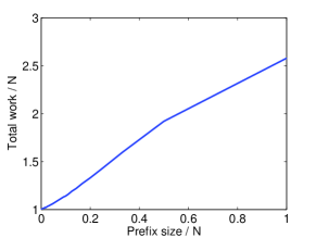
(a) Total work done vs. prefix size on a random graph ($n=10^{7},m=5\times 10^{7}$)

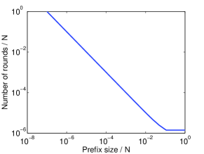
(b) Number of rounds vs. prefix size on a random graph ($n=10^{7},m=5\times 10^{7}$) in log-log scale

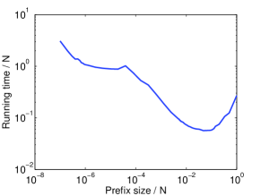
(c) Running time (32 processors) vs. prefix size on a random graph ($n=10^{7},m=5\times 10^{7}$) in log-log scale

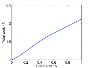
(d) Total work done vs. prefix size on a rMat graph ($n=2^{24},m=5\times 10^{7}$)

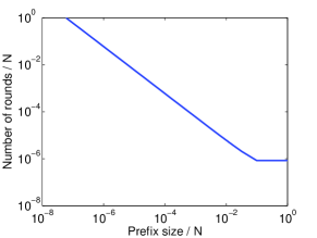
(e) Number of rounds vs. prefix size on a rMat graph ($n=2^{24},m=5\times 10^{7}$) in log-log scale

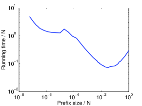
(f) Running time (32 processors) vs. prefix size on a rMat graph ($n=2^{24},m=5\times 10^{7}$) in log-log scale

Figure 1: Plots showing the tradeoff between various properties and the prefix size in maximal independent set.

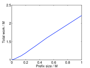
(a) Total work done vs. prefix size on a random graph ($n=10^{7},m=5\times 10^{7}$)

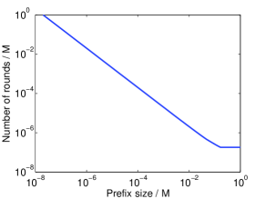
(b) Number of rounds vs. prefix size on a random graph ($n=10^{7},m=5\times 10^{7}$) in log-log scale

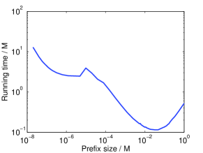
(c) Running time (32 processors) vs. prefix size on a random graph ($n=10^{7},m=5\times 10^{7}$) in log-log scale

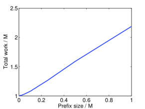
(d) Total work done vs. prefix size on a rMat graph ($n=2^{24},m=5\times 10^{7}$)

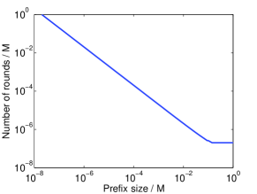
(e) Number of rounds vs. prefix size on a rMat graph ($n=2^{24},m=5\times 10^{7}$) in log-log scale

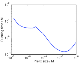
(f) Running time (32 processors) vs. prefix size on a rMat graph ($n=2^{24},m=5\times 10^{7}$) in log-log scale

Figure 2: Plots showing the tradeoff between various properties and the prefix size in maximal matching.

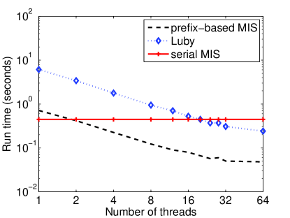
(a) Running time vs. number of threads on a random graph ($n=10^{7},m=5\times 10^{7}$) in log-log scale

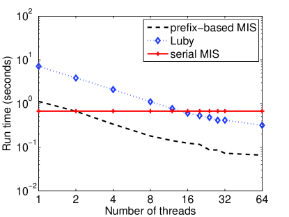
(b) Running time vs. number of threads on a rMat graph ($n=2^{24},m=5\times 10^{7}$) in log-log scale

Figure 3: Plots showing the running time vs. number of threads for the different MIS algorithms on a 32-core machine (with hyper-threading).

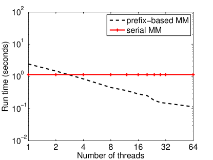
(a) Running time vs. number of threads on a random graph ($n=10^{7},m=5\times 10^{7}$) in log-log scale

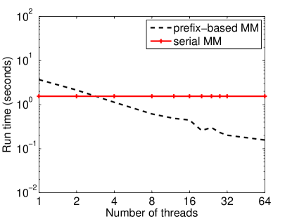
(b) Running time vs. number of threads on a rMat graph ($n=2^{24},m=5\times 10^{7}$) in log-log scale

Figure 4: Plots showing the running time vs. number of threads for the different MM algorithms on a 32-core machine (with hyper-threading).

References

- [1] Noga Alon, László Babai, and Alon Itai. A fast and simple randomized parallel algorithm for the maximal independent set problem. J. Algorithms, 7:567–583, December 1986.
- [2] Guy E. Blelloch, Jeremy T. Fineman, Phillip B. Gibbons, and Julian Shun. Internally deterministic algorithms can be fast. In Proceedings of Principles and Practice of Parallel Programming, PPoPP, 2012.
- [3] Robert L. Bocchino, Vikram S. Adve, Sarita V. Adve, and Marc Snir. Parallel programming must be deterministic by default. In Usenix HotPar, 2009.
- [4] Neil J. Calkin and Alan M. Frieze. Probabilistic analysis of a parallel algorithm for finding maximal independent sets. Random Struct. Algorithms, 1(1):39–50, 1990.
- [5] Deepayan Chakrabarti, Yiping Zhan, and Christos Faloutsos. R-MAT: A recursive model for graph mining. In SIAM SDM, 2004.
- [6] Stephen A. Cook. A taxonomy of problems with fast parallel algorithms. Inf. Control, 64:2–22, March 1985.
- [7] Don Coppersmith, Prabhakar Raghavan, and Martin Tompa. Parallel graph algorithms that are effcient on average. Inf. Comput., 81:318–333, June 1989.
- [8] Thomas H. Cormen, Charles E. Leiserson, Ronald L. Rivest, and Clifford Stein. Introduction to Algorithms (3. ed.). MIT Press, 2009.
- [9] Andrew V. Goldberg, Serge A. Plotkin, and Gregory E. Shannon. Parallel symmetry-breaking in sparse graphs. In SIAM J. Disc. Math, pages 315–324, 1987.
- [10] Mark Goldberg and Thomas Spencer. Constructing a maximal independent set in parallel. SIAM Journal on Discrete Mathematics, 2:322–328, August 1989.
- [11] Mark Goldberg and Thomas Spencer. A new parallel algorithm for the maximal independent set problem. SIAM Journal on Computing, 18:419–427, April 1989.
- [12] Mark K. Goldberg. Parallel algorithms for three graph problems. Congressus Numerantium, 54:111–121, 1986.
- [13] Raymond Greenlaw, James H. Hoover, and Walter L. Ruzzo. Limits to Parallel Computation: P-Completeness Theory. Oxford University Press, USA, April 1995.
- [14] Amos Israeli and A. Itai. A fast and simple randomized parallel algorithm for maximal matching. Inf. Process. Lett., 22:77–80, February 1986.
- [15] Amos Israeli and Y. Shiloach. An improved parallel algorithm for maximal matching. Inf. Process. Lett., 22:57–60, February 1986.
- [16] Richard M. Karp and Avi Wigderson. A fast parallel algorithm for the maximal independent set problem. In STOC, 1984.
- [17] Michael Luby. A simple parallel algorithm for the maximal independent set problem. SIAM J. Comput., 15:1036–1055, November 1986.