Analytical solutions to the spin-1 Bose-Einstein condensates

Abstract

We analytically solve the one-dimensional coupled Gross-Pitaevskii equations which govern the motion of $F=1$ spinor Bose-Einstein condensates. The nonlinear density-density interactions are decoupled by making use of the unique properties of the Jacobian elliptical functions. Several types of complex stationary solutions are deduced. Furthermore, exact non-stationary solutions to the time-dependent Gross-Pitaevskii equations are constructed by making use of the spin-rotational symmetry of the Hamiltonian. The spin-polarizations exhibit kinked configurations. Our method is applicable to other coupled nonlinear systems.

I Introduction

Most Bose-Einstein condensates (BECs) of dilute atomic gases realized thus far have internal degrees of freedom arising from spins. The spinor BECs have been realized in the optical traps which confine the atoms regardless of their spin hyperfine states. The direction of the spin can change dynamically due to collisions between the atomsBarrett ; Gorlitz ; Leanhardt . The spinor BECs exhibit a rich variety of magnetic phenomena. They give rise to phenomena that are not present in the single component BECs, including magnetic crystallization, spin textures as well as fractional vorticesStenger ; Miesner ; Kobayashi . Moreover, there exists an interplay between superfluidity and magnetism due to the spin-gauge symmetry. A ferromagnetic BEC spontaneously creates a supercurrent as the spin is locally rotatedUeda ; Kawaguchi .

A spinor condensate formed by atoms with spin $F=1$ is described by a macroscopic wave function with three components $\Psi=(\psi_{+1},\psi_{0},\psi_{-1})^{T}$. The mean-field Hamiltonian is expressed asHo ; Chang

$$H=\int d\textbf{r} \{\sum_{m=-1}^{1}\psi_{m}^{*}[-\frac{\hbar^{2}}{2M}\bigtriangledown^{2}+V(\textbf{r})]\psi_{m}$$ (1)

$$+\frac{\bar{c}_{0}}{2}n_{tot}^{2}+\frac{\bar{c}_{2}}{2}|\textbf{F}|^{2}\},$$

where the spin-polarization vector $\textbf{F}=\psi_{m}^{*}\hat{\textbf{F}}_{mn}\psi_{n}$ with $\hat{\textbf{F}}^{i}$ ($i=x,y,z$) the rotational matrices. The coupling constants $\bar{c}_{0}=(g_{0}+2g_{2})/3$ and $\bar{c}_{2}=(g_{2}-g_{0})/3$, with $g_{F}$ relating to the $s$-wave scattering length of the total spin-$F$ channel as $g_{F}=4\pi\hbar^{2}a_{F}/M$. $n_{tot}=|\psi_{1}|^{2}+\psi_{0}|^{2}+|\psi_{-1}|^{2}$ is the particle density and $V(\textbf{r})$ is the external potential. The full symmetry of the Hamiltonian is $SO(3)\times U(1)$. The energies are degenerate for an arbitrary state $\Psi$ and its globally spin-rotational states $\Psi^{\prime}=U\Psi$, where $U$ is the three-dimensional rotational matrix in the spin space which is expressed by the Euler angles as $U(\alpha,\beta,\gamma)=e^{-i\hat{F}_{z}\alpha}e^{-i\hat{F}_{y}\beta}e^{-i\hat{F}_{z}\gamma}$. In the ground state, the symmetry is spontaneously broken in several different ways, leading to a number of possible phasesHo ; Chang ; Murata ; Imambekov .

We are concerned with the quasi-one-dimensional (1D) $F=1$ BEC in a uniform external potential ($V(\textbf{r})=0$). The dynamical motions of the spinor wavefunctions are governed by $i\partial_{t}\psi_{m}=\delta H/\delta\psi_{m}^{*}$, which are explicitly written as the coupled nonlinear Gross-Pitaevskii equations (GPEs),

$$i\hbar\partial_{t}\psi_{m}=[-\frac{\hbar^{2}}{2M}\partial_{x}^{2}+c_{0}n_{tot}\\ +c_{2}(\Psi^{\dagger}\hat{F}^{i}\Psi)\hat{F}_{mn}^{i}]\psi_{n},$$ (2)

where $c_{0}=\bar{c}_{0}/2a_{\perp}^{2}$ and $c_{2}=\bar{c}_{2}/2a_{\perp}^{2}$ are the reduced coupling constants with $a_{\perp}$ the transverse width of the quasi-1D system. The GPE was first introduced for unrelated problemsGross ; Ginzburg . It has been proved to be effective in describing many phenomena observed in the dilute gas BECsDalfovo and other quantum systemsCoen ; N.Z. .

There is a lot of theoretical works that numerically solve Eqs.(2) or the corresponding stationary equationsLi ; Zhang ; Nistazakis . Nevertheless, it is of great interest if analytical solutions can be acquired. By using the so-called inverse scattering transformation method and the function transformation methodGardner ; Sedawy ; Uchiyama ; Ieda , some special solutions are obtained. The soliton solutions are obtained by the similar transformation method for systems with appropriate time or spatial variations in the coupling constantBeitia ; Theocharis ; Avelar ; Wang . Various approximations are employed to study the solitons such as bright and dark solitons in the $F=1$ spinor BECsCarr ; Bradley ; LLi ; Yan .

However, exact analytical solutions to the spinor BECs, especially in non-soliton forms, are absent in literature. Attempts in this direction are usually frustrated by the complexity of the nonlinear couplings. The challenges are two-fold: one is the nonlinear density-density interactions which is associated with the $c_{0}$ term, while the other is the spin-exchange couplings between the hyperfine states which is associated with the $c_{2}$ term. In this paper, we present several types of exact solutions by decoupling the nonlinear density-density interactions. The solutions are expressed by combinations of the Jacobian elliptic functions. Furthermore, the exact non-stationary solutions are naturally produced by making using of the spin-rotational symmetry of the Hamiltonian.

The paper is organized as follows. Section II describes exact stationary solutions to the coupled GPEs. In Sec. III, we present the associated non-stationary solutions. Section IV contains a summary of the main results.

II Stationary solutions

The most general form of the stationary equations corresponding to Eqs.(2) are obtained by substituting

$$\left(\begin{array}[]{c}\psi_{1}(x,t)\\ \psi_{0}(x,t)\\ \psi_{-1}(x,t)\\ \end{array}\right)\rightarrow\left(\begin{array}[]{c}\psi_{1}(x)e^{-i(\mu+\mu_{1})t}\\ \psi_{0}(x)e^{-i\mu t}\\ \psi_{-1}(x)e^{-i(\mu-\mu_{1})t}\\ \end{array}\right),$$ (3)

which give rise to

$$(\mu+\mu_{1})\psi_{1} = [-\frac{1}{2}\partial_{x}^{2}+(c_{0}+c_{2})(|\psi_{1}|^{2}+|\psi_{0}|^{2})$$

$$+(c_{0}-c_{2})|\psi_{-1}|^{2}]\psi_{1}+c_{2}\psi_{0}^{2}\psi_{-1}^{*},$$

$$\mu\psi_{0} = [-\frac{1}{2}\partial_{x}^{2}+(c_{0}+c_{2})(|\psi_{1}|^{2}+|\psi_{-1}|^{2})$$

$$+c_{0}|\psi_{0}|^{2}]\psi_{0}+2c_{2}\psi_{0}^{*}\psi_{1}\psi_{-1},$$

$$(\mu-\mu_{1})\psi_{-1} = [-\frac{1}{2}\partial_{x}^{2}+(c_{0}+c_{2})(|\psi_{1}|^{2}+|\psi_{0}|^{2})$$ (4)

$$+(c_{0}-c_{2})|\psi_{1}|^{2}]\psi_{-1}+c_{2}\psi_{0}^{2}\psi_{1}^{*}.$$

Here we have chosen $\hbar=M=1$ as the units for convenience. The coupling constants $c_{0}$ and $c_{2}$, or $a_{0}$ and $a_{2}$ are treated as free parameters. It is notable that the non-zero parameter $\mu_{1}$ plays an important role in the seeking of analytical solutions.

The periodic boundary conditions

$$\psi_{m}(1)=\psi_{m}(0),\hskip 11.38109pt\psi_{m}^{\prime}(1)=\psi_{m}^{\prime}(0),$$ (5)

are adopted in our calculation. In the following, we present four types of complex solutions to the Eqs.(4). All solutions have been numerically verified to be stationary by the dynamical evolution Eqs.(2).

Type A. Solution of the cn-sn form

Here, we focus on solutions with $\psi_{0}=0$. At the same time, the nonlinear density-density interactions between different components are decoupled by using the unique properties of the Jacobian elliptical functions. We first consider the following form of solution,

$$\left(\begin{array}[]{c}\psi_{1}\\ \psi_{0}\\ \psi_{-1}\\ \end{array}\right)=\left(\begin{array}[]{c}f(x)e^{i\theta(x)}\\ 0\\ D\textrm{sn}(kx,m)\\ \end{array}\right),$$ (6)

where $f(x)=\sqrt{A+B\textrm{cn}^{2}(kx,m)}$. $A$, $B$ and $D$ are real constants. sn and cn are the Jacobian elliptical functions and $k=4jK(m)$ with $m$ the modulus $(0<m<1)$. In this paper we always take the number of periods $j=2$ as examples. In order to decouple the nonlinear equations (4), we make use of the property $\textrm{sn}^{2}+\textrm{cn}^{2}=1$ to have

$$|\psi_{-1}|^{2}=(1-\frac{|\psi_{1}|^{2}-A}{B})D^{2},\ \ |\psi_{1}|^{2}=A+B(1-\frac{|\psi_{-1}|^{2}}{D^{2}}).$$ (7)

Substituting the relations into the stationary Eqs.(4), we obtain the decoupled equations

$$\tilde{\mu}_{m}\psi_{m}=-\frac{1}{2}\psi_{m}^{\prime\prime}+\tilde{\gamma}_{m}|\psi_{m}|^{2}\psi_{m},\ \ (m=0,\pm 1)$$ (8)

where the effective chemical potentials $\tilde{\mu}_{m}$ and interacting constants $\tilde{\gamma}_{m}$ are defined as

$$\left\{\begin{array}[]{ll}\tilde{\mu}_{1}=\mu+\mu_{1}-(c_{0}-c_{2})(A+B)\frac{D^{2}}{B},\\ \tilde{\gamma}_{1}=(c_{0}+c_{2})-(c_{0}-c_{2})\frac{D^{2}}{B},\end{array}\right.$$ (9)

and

$$\left\{\begin{array}[]{ll}\tilde{\mu}_{-1}=\mu-\mu_{1}-(c_{0}-c_{2})(A+B),\\ \tilde{\gamma}_{-1}=(c_{0}+c_{2})-(c_{0}-c_{2})\frac{B}{D^{2}}.\end{array}\right.$$ (10)

The Eqs.(8) can be self-consistently solved as

$$B=-\frac{m^{2}k^{2}}{\tilde{\gamma}_{1}},$$

$$A=\frac{4\mu_{1}+3m^{2}k^{2}+4(c_{0}-c_{2})B}{2(c_{0}+2c_{2})},$$

$$D^{2}=\frac{m^{2}k^{2}}{\tilde{\gamma}_{-1}},$$ (11)

with

$$\mu=\frac{6c_{0}A+k^{2}(2-m^{2})}{4},$$

$$\tilde{\gamma}_{1}=\tilde{\gamma}_{-1}=2c_{0}.$$ (12)

It implies that the effective nonlinear interactions in each component should be repulsive ($\tilde{\gamma}_{m}>0$), which impose a constraint on the value of the coupling constants $c_{0}$.

The phase $\theta(x)$ in Eqs.(6) is given by

$$\theta(x)=\int_{0}^{x}\frac{\alpha_{1}}{f(\xi)^{2}}d\xi,$$ (13)

where $\alpha_{1}=\pm(2\tilde{\mu}_{1}A^{2}-2\tilde{\gamma}_{1}A^{3}+k^{2}(1-m^{2})AB)^{\frac{1}{2}}$ is an integral constant. The periodic boundary conditions (5) require that the amplitudes and phase respectively satisfy

$$f(1)=f(0),\hskip 11.38109pt\theta(1)-\theta(0)=2j\pi\times n,$$ (14)

where $n$ is an integer. The periodic condition for the phase $\theta(x)$ can be satisfied by properly adjusting the modulus $m$ of the Jacobian elliptic functions.

Figure 1: The phase (a) and the density (b) distributions for solution (6) with $n=2$, $m=0.78$. The physical parameters are $c_{0}=4$, $c_{2}=2$, $\mu=422.4701$, and $\mu_{1}=150$. (c) The distribution of the spin-polarization.

Figure 1 display the distributions of some relevant physical quantities for the solution (6). We have chosen $c_{0}=4$, $c_{2}=2$, $\mu=422.4701$ and $\mu_{1}=150$. Fig.1(a) is the phase distribution with $j=2$, $n=2$ and $m=0.78$. Fig.1(b) is the density distributions of each hyperfine state. The spin-polarization is shown in Fig.1(c) which exhibits a kinked configuration.

Type B. Solution of the sn-cn form

We take the following form of solutions to the stationary equations (4).

$$\left(\begin{array}[]{c}\psi_{1}\\ \psi_{0}\\ \psi_{-1}\\ \end{array}\right)=\left(\begin{array}[]{c}f(x)e^{i\theta(x)}\\ 0\\ D\textrm{cn}(kx,m)\\ \end{array}\right),$$ (15)

where $f(x)=\sqrt{A+B\textrm{sn}^{2}(kx,m)}$. $A$, $B$ and $D$ are real constants. One has

$$|\psi_{-1}|^{2}=(A+B-|\psi_{1}|^{2})\frac{D^{2}}{B},\ \ |\psi_{1}|^{2}=A+B-\frac{B}{D^{2}}|\psi_{-1}|^{2}.$$ (16)

By the same means in the previous subsection, we decouple the Eqs.(4) and derive the effective chemical potentials $\tilde{\mu}_{m}$ and interacting constants $\tilde{\gamma}_{m}$ as

$$\left\{\begin{array}[]{ll}\tilde{\mu}_{1}=\mu+\mu_{1}-(c_{0}-c_{2})(A+B)\frac{D^{2}}{B},\\ \tilde{\gamma}_{1}=(c_{0}+c_{2})-(c_{0}-c_{2})\frac{D^{2}}{B},\end{array}\right.$$ (17)

and

$$\left\{\begin{array}[]{ll}\tilde{\mu}_{-1}=\mu-\mu_{1}-(c_{0}-c_{2})(A+B),\\ \tilde{\gamma}_{-1}=(c_{0}+c_{2})-(c_{0}-c_{2})\frac{B}{D^{2}}.\end{array}\right.$$ (18)

With this form of solutions, the decoupled Eqs.(8) are self-consistently solved as

$$B=\frac{m^{2}k^{2}}{\tilde{\gamma}_{1}},$$

$$A=\frac{4\mu_{1}-3m^{2}k^{2}+4(c_{0}-c_{2})B}{2(c_{0}+2c_{2})},$$

$$D^{2}=-\frac{m^{2}k^{2}}{\tilde{\gamma}_{-1}},$$

with

$$\mu=\frac{6c_{0}A+k^{2}(2-m^{2})}{4},$$

$$\tilde{\gamma}_{1}=\tilde{\gamma}_{-1}=2c_{0}.$$ (20)

One observes that $\tilde{\gamma}_{m}<0$ which imply the effective interactions in each component should be attractive. The phase is

$$\theta(x)=\int_{0}^{x}\frac{\alpha_{1}}{f(\xi)^{2}}d\xi,$$ (21)

where $\alpha_{1}=\pm(2\tilde{\mu}_{1}A^{2}-2\tilde{\gamma}_{1}A^{3}+k^{2}AB)^{\frac{1}{2}}$ is an integral constant. The amplitudes and the phase should satisfy the periodic boundary conditions (5), which can be realized by scanning the modulus $m$.

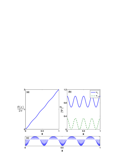
Figure 2: The same as in Fig.3 for the solution (15) with $n=1$ and $m=0.29$. The physical parameters are $c_{0}=-2$, $c_{2}=6$, $\mu=47.6088$, and $\mu_{1}=35$.

Figure 2 display the distributions of the relevant physical quantities for the solution (15). We have chosen $c_{0}=-2$, $c_{2}=6$, $\mu=47.6088$ and $\mu_{1}=35$. $n=1$ and the value $m=0.29$ is numerically scanned.

Type C. Solution of the sn-dn form

we take the following ansatz as the most solution of the nonlinear Eqs.(4).

$$\left(\begin{array}[]{c}\psi_{1}\\ \psi_{0}\\ \psi_{-1}\\ \end{array}\right)=\left(\begin{array}[]{c}f(x)e^{i\theta(x)}\\ 0\\ D\textrm{dn}(kx,m)\\ \end{array}\right),$$ (22)

where $f(x)=\sqrt{A+B\textrm{sn}^{2}(kx,m)}$. $A$, $B$ and $D$ are real constants. One has

$$|\psi_{-1}|^{2}=\frac{D^{2}}{B}(B+m^{2}A-m^{2}|\psi_{1}|^{2}),\ \ |\psi_{1}|^{2}=A+\frac{B}{m^{2}}-\frac{B}{m^{2}D^{2}}|\psi_{-1}|^{2}.$$ (23)

Similarly, the decoupled equations (8) contain the effective chemical potentials $\tilde{\mu}_{m}$ and interacting constants $\tilde{\gamma}_{m}$ as

$$\left\{\begin{array}[]{ll}\tilde{\mu}_{1}=\mu+\mu_{1}-(c_{0}-c_{2})(m^{2}A+B)\frac{D^{2}}{B},\\ \tilde{\gamma}_{1}=(c_{0}+c_{2})-(c_{0}-c_{2})\frac{m^{2}D^{2}}{B},\end{array}\right.$$ (24)

and

$$\left\{\begin{array}[]{ll}\tilde{\mu}_{-1}=\mu-\mu_{1}-(c_{0}-c_{2})(A+\frac{B}{m^{2}}),\\ \tilde{\gamma}_{-1}=(c_{0}+c_{2})-(c_{0}-c_{2})\frac{B}{m^{2}D^{2}}.\end{array}\right.$$ (25)

This form of solutions to the decoupled Eqs.(8) are self-consistently solved as

$$B=\frac{m^{2}k^{2}}{\tilde{\gamma}_{1}},$$

$$A=\frac{4\mu_{1}-3k^{2}+4(c_{0}-c_{2})\frac{B}{m^{2}}}{2(c_{0}+2c_{2})},$$

$$D^{2}=-\frac{k^{2}}{\tilde{\gamma}_{-1}},$$ (26)

with

$$\mu=\frac{6c_{0}A-k^{2}(1-2m^{2})}{4},$$

$$\tilde{\gamma}_{1}=\tilde{\gamma}_{-1}=2c_{0}.$$ (27)

The negative values of $\tilde{\gamma}_{m}<0$ for this form of complex solution imply effective attractive interactions in each component. The phase is

$$\theta(x)=\int_{0}^{x}\frac{\alpha_{1}}{f(\xi)^{2}}d\xi,$$ (28)

where $\alpha_{1}=\pm(2\tilde{\mu}_{1}A^{2}-2\tilde{\gamma}_{1}A^{3}+k^{2}AB)^{\frac{1}{2}}$ is an integral constant. The periodic boundary conditions are satisfied by properly adjusting the modulus $m$.

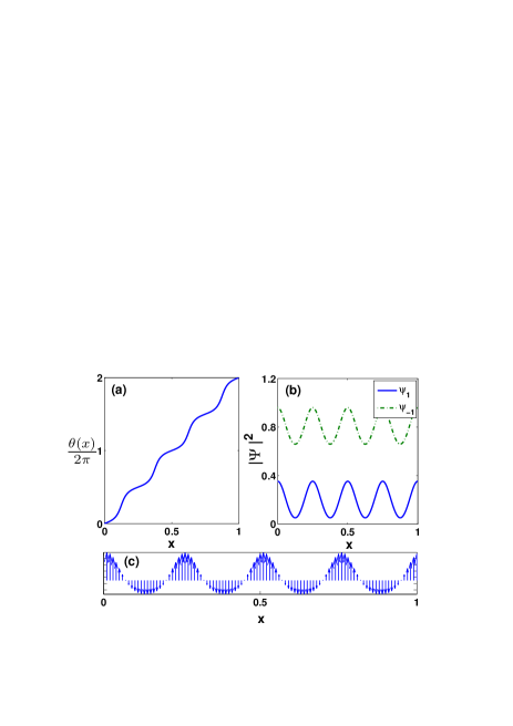
Figure 3: The phase (a) and the density (b) distributions for solution (22) with $n=1$, $m=0.56$. The physical parameters are $c_{0}=-2$, $c_{2}=4$, $\mu=-70.008$, and $\mu_{1}=90$. (c) The distribution of the spin-polarization.

Figure 3 display the distributions of the phase (Fig.3a), the density (Fig.3b) for the solution (22). The physical parameters are chosen as $c_{0}=-2$, $c_{2}=4$, $\mu=-70.008$, and $\mu_{1}=90$, whereas $n=1$ and the value $m=0.56$ is numerically scanned. The spin polarization of this solution is shown in Fig.3(c).

Type D. Solution of the dn-sn form

Consider the following form of solutions to the nonlinear stationary Eqs.(4),

$$\left(\begin{array}[]{c}\psi_{1}\\ \psi_{0}\\ \psi_{-1}\\ \end{array}\right)=\left(\begin{array}[]{c}f(x)e^{i\theta(x)}\\ 0\\ D\textrm{sn}(kx,m)\\ \end{array}\right),$$ (29)

where $f(x)=\sqrt{A+B\textrm{dn}^{2}(kx,m)}$. One has

$$|\psi_{-1}|^{2}=(A+B-|\psi_{1}|^{2})\frac{D^{2}}{m^{2}B},\ \ |\psi_{1}|^{2}=A+B-\frac{m^{2}B}{D^{2}}|\psi_{-1}|^{2}.$$ (30)

The stationary equations (4) are decouple into (8), with the effective chemical potentials $\tilde{\mu}_{m}$ and interacting constants $\tilde{\gamma}_{m}$,

$$\left\{\begin{array}[]{ll}\tilde{\mu}_{1}=\mu+\mu_{1}-(c_{0}-c_{2})(A+B)\frac{D^{2}}{m^{2}B},\\ \tilde{\gamma}_{1}=(c_{0}+c_{2})-(c_{0}-c_{2})\frac{D^{2}}{m^{2}B},\end{array}\right.$$ (31)

and

$$\left\{\begin{array}[]{ll}\tilde{\mu}_{-1}=\mu-\mu_{1}-(c_{0}-c_{2})(A+B),\\ \tilde{\gamma}_{-1}=(c_{0}+c_{2})-(c_{0}-c_{2})\frac{m^{2}B}{D^{2}}.\end{array}\right.$$ (32)

This form of solutions to the decoupled Eqs.(8) are self-consistently solved as

$$B=-\frac{k^{2}}{\tilde{\gamma}_{1}},$$

$$A=\frac{4\mu_{1}+3k^{2}+4(c_{0}-c_{2})B}{2(c_{0}+2c_{2})},$$

$$D^{2}=\frac{m^{2}k^{2}}{\tilde{\gamma}_{-1}},$$

with

$$\mu=\frac{6c_{0}A+k^{2}(2m^{2}-1)}{4},$$

$$\tilde{\gamma}_{1}=\tilde{\gamma}_{-1}=2c_{0}.$$ (34)

The positive values of $\tilde{\gamma}_{m}>0$ for this form of solution imply that effective interactions in each component are repulsive. The phase is

$$\theta(x)=\int_{0}^{x}\frac{\alpha_{1}}{f(\xi)^{2}}d\xi,$$ (35)

where $\alpha_{1}=\pm(2\tilde{\mu}_{1}A^{2}-2\tilde{\gamma}_{1}A^{3}+k^{2}(m^{2}-1)AB)^{\frac{1}{2}}$ is an integral constant. Accordingly, the amplitudes and phase should satisfy the periodic boundary conditions (5).

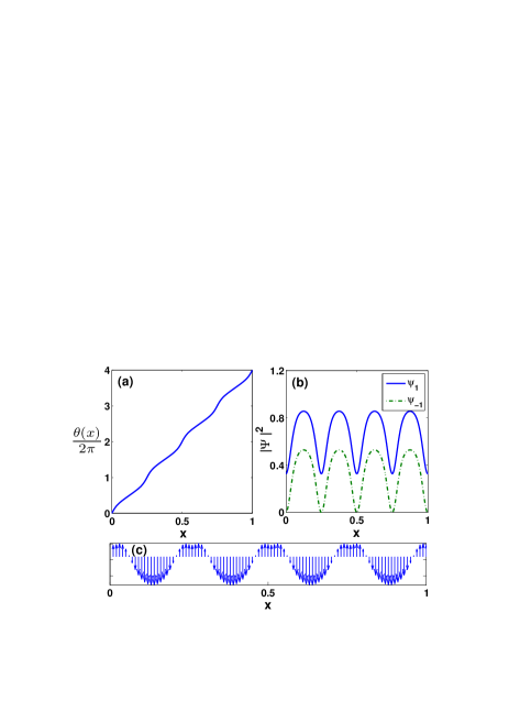
Figure 4: The same as in Fig.3 for the solution (29) with $n=2$ and $m=0.95$. The physical parameters are $c_{0}=8$, $c_{2}=2$, $\mu=588.3927$, and $\mu_{1}=90$.

Figure 4 display the distributions of the phase (Fig.4a), the density (Fig.4b) for the solution (29). The physical parameters are chosen as $c_{0}=8$, $c_{2}=2$, $\mu=588.3927$, and $\mu_{1}=90$, whereas $n=2$ and the value $m=0.95$ is numerically scanned. The spin-polarization of this solution is shown in Fig.4(c).

III Non-stationary solutions

Suppose $\Psi(x)=(\psi_{1}(x),\psi_{0}(x),\psi_{-1}(x))^{T}$ is a stationary solution to the equations (4), the full spatial and temporal form of the solution is written by adding the time factor,

$$\Psi(x,t)=\left(\begin{array}[]{c}\psi_{1}(x)e^{-i(\mu+\mu_{1})t}\\ \psi_{0}(x)e^{-i\mu t}\\ \psi_{-1}(x)e^{-i(\mu-\mu_{1})t}\\ \end{array}\right),$$ (36)

Since the Hamiltonian (1) has the $SO(3)$ spin-rotational symmetry, then $\Psi^{\prime}(x,t)=U\Psi(x,t)$ is a solution to the equations of motion (2). Here $U$ is the three-dimensional rotational matrix in the spin space expressed by the three Euler angles $(\alpha,\beta,\gamma)$,

$$U=\left(\begin{array}[]{ccc}e^{-i(\alpha+\gamma)}\cos^{2}\frac{\beta}{2}&-\frac{1}{\sqrt{2}}e^{-i\alpha}\sin\beta&e^{-i(\alpha-\gamma)}\sin^{2}\frac{\beta}{2}\\ \frac{1}{\sqrt{2}}e^{-i\gamma}\sin\beta&\cos\beta&-\frac{1}{\sqrt{2}}e^{i\gamma}\sin\beta\\ e^{i(\alpha-\gamma)}\sin^{2}\frac{\beta}{2}&\frac{1}{\sqrt{2}}e^{i\alpha}\sin\beta&e^{i(\alpha+\gamma)}\cos^{2}\frac{\beta}{2}\\ \end{array}\right).$$ (37)

Given the non-zero value of $\mu_{1}$, we observe that $\Psi^{\prime}(x,t)$ is an exact non-stationary solution. It is notable that $\Psi^{\prime}(x,0)$ is no longer the stationary solution to the Eqs.(4). In this section, we construct the corresponding non-stationary solutions associated to the stationary solutions obtained in the previous section. We will fix the Euler angles $\alpha=7\pi/13$, $\beta=\pi/4$ and $\gamma=\pi/11$.

III.1 Solution associated to Type A

By applying the spin-rotational transformation to the stationary solution (6), we obtain the the non-stationary solution as follows:

$$\Psi^{\prime}(x,t)=\left(\begin{array}[]{c}\psi_{1}e^{-i(\mu+\mu_{1})t}e^{-i(\alpha+\gamma)}\cos^{2}(\frac{\beta}{2})+\psi_{-1}e^{-i(\mu-\mu_{1})t}e^{-i(\alpha-\gamma)}\sin^{2}(\frac{\beta}{2})\\ \psi_{1}e^{-i(\mu+\mu_{1})t}e^{-i\gamma}\sin\beta/\sqrt{2}-\psi_{-1}e^{-i(\mu-\mu_{1})t}e^{i\gamma}\sin\beta/\sqrt{2}\\ \psi_{1}e^{-i(\mu+\mu_{1})t}e^{i(\alpha-\gamma)}\sin^{2}(\frac{\beta}{2})+\psi_{-1}e^{-i(\mu-\mu_{1})t}e^{i(\alpha+\gamma)}\cos^{2}(\frac{\beta}{2})\\ \end{array}\right)$$ (41)

where $\psi_{1}=\sqrt{A+B\textrm{cn}^{2}(kx,m)}e^{i\theta(x)}$ and $\psi_{-1}=D\textrm{sn}(kx,m)$. The density of each component $n_{i}(x,t)=|\psi_{i}^{\prime}(x,t)|^{2}$, $(i=1,2,3)$ is given by

$$n_{1}(x,t) = |\psi_{1}|^{2}(\cos^{2}\frac{\beta}{2})^{2}+|\psi_{-1}|^{2}(\sin^{2}\frac{\beta}{2})^{2}+2\sqrt{A+B\textrm{cn}^{2}}D\textrm{sn}\sin^{2}\frac{\beta}{2}\cos^{2}\frac{\beta}{2}\cos(2\mu_{1}t-2\gamma+\theta),$$

$$n_{0}(x,t) = |\psi_{1}|^{2}\sin^{2}\beta/2+|\psi_{-1}|^{2}\sin^{2}\beta/2-\sqrt{A+B\textrm{cn}^{2}}D\textrm{sn}\sin^{2}\beta\cos(2\mu_{1}t-2\gamma+\theta),$$

$$n_{-1}(x,t) = |\psi_{1}|^{2}(\sin^{2}\frac{\beta}{2})^{2}+|\psi_{-1}|^{2}(\cos^{2}\frac{\beta}{2})^{2}+2\sqrt{A+B\textrm{cn}^{2}}D\textrm{sn}\sin^{2}\frac{\beta}{2}\cos^{2}\frac{\beta}{2}\cos(2\mu_{1}t-2\gamma+\theta).$$

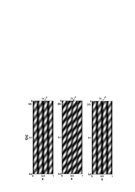
Figure 5: The density distribution of the non-stationary solution (41). The parameters are the same as in Fig.1.

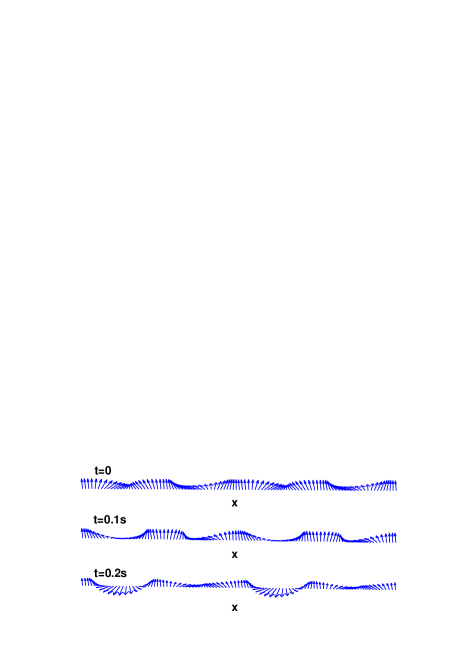
Figure 6: Snapshots of the spin-polarization distributions of the non-stationary solutions (41) at $t=0s,t=0.1s$ and $t=0.2s$, respectively.

III.2 Solution associated to Type B

By applying the spin-rotational transformation to the stationary solution (15), we obtain the non-stationary solution as follows:

$$\Psi^{\prime}(x,t)=\left(\begin{array}[]{c}\psi_{1}e^{-i(\mu+\mu_{1})t}e^{-i(\alpha+\gamma)}\cos^{2}(\frac{\beta}{2})+\psi_{-1}e^{-i(\mu-\mu_{1})t}e^{-i(\alpha-\gamma)}\sin^{2}(\frac{\beta}{2})\\ \psi_{1}e^{-i(\mu+\mu_{1})t}e^{-i\gamma}\sin\beta/\sqrt{2}-\psi_{-1}e^{-i(\mu-\mu_{1})t}e^{i\gamma}\sin\beta/\sqrt{2}\\ \psi_{1}e^{-i(\mu+\mu_{1})t}e^{i(\alpha-\gamma)}\sin^{2}(\frac{\beta}{2})+\psi_{-1}e^{-i(\mu-\mu_{1})t}e^{i(\alpha+\gamma)}\cos^{2}(\frac{\beta}{2})\\ \end{array}\right),$$ (46)

where $\psi_{1}=\sqrt{A+B\textrm{sn}^{2}(kx,m)}e^{i\theta(x)}$ and $\psi_{-1}=D\textrm{cn}(kx,m)$. The density of each component $n_{i}(x,t)=|\psi_{i}^{\prime}(x,t)|^{2}$, $(i=1,2,3)$ is given by

$$n_{1}(x,t) = |\psi_{1}|^{2}(\cos^{2}\frac{\beta}{2})^{2}+|\psi_{-1}|^{2}(\sin^{2}\frac{\beta}{2})^{2}+2\sqrt{A+B\textrm{sn}^{2}}D\textrm{cn}\sin^{2}\frac{\beta}{2}\cos^{2}\frac{\beta}{2}\cos(2\mu_{1}t-2\gamma+\theta),$$

$$n_{0}(x,t) = |\psi_{1}|^{2}\sin^{2}\beta/2+|\psi_{-1}|^{2}\sin^{2}\beta/2-\sqrt{A+B\textrm{sn}^{2}}D\textrm{cn}\sin^{2}\beta\cos(2\mu_{1}t-2\gamma+\theta),$$

$$n_{-1}(x,t) = |\psi_{1}|^{2}(\sin^{2}\frac{\beta}{2})^{2}+|\psi_{-1}|^{2}(\cos^{2}\frac{\beta}{2})^{2}+2\sqrt{A+B\textrm{sn}^{2}}D\textrm{cn}\sin^{2}\frac{\beta}{2}\cos^{2}\frac{\beta}{2}\cos(2\mu_{1}t-2\gamma+\theta).$$

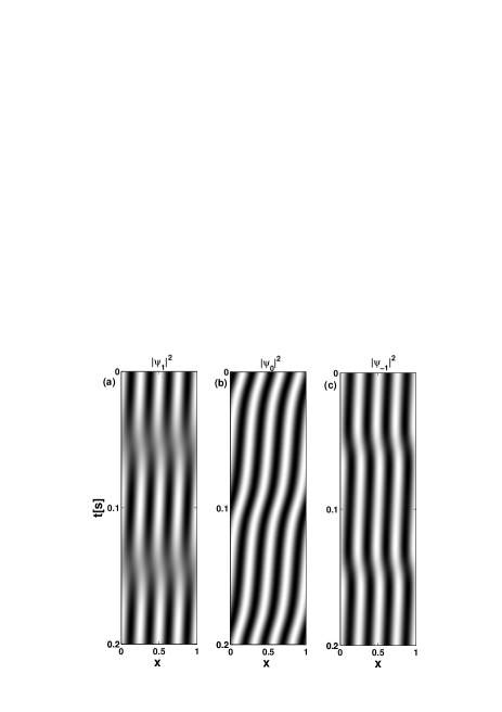
Figure 7: The density distribution of the non-stationary solution (46). The parameters are the same as in Fig.2.

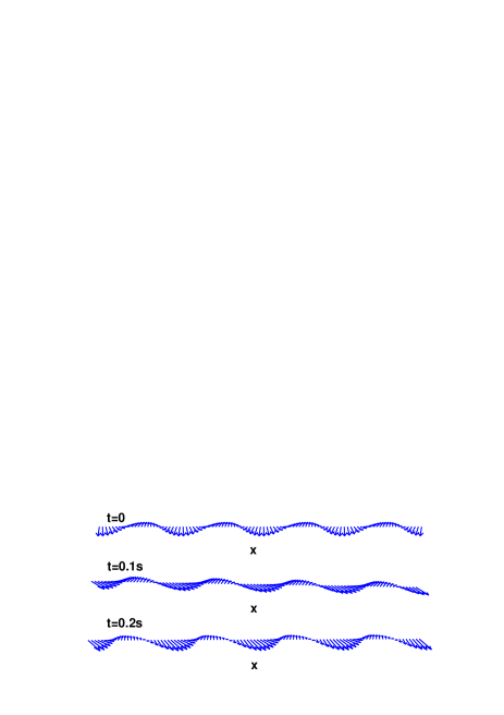
Figure 8: Snapshots of the spin-polarization distributions of the non-stationary solutions (46) at $t=0s,t=0.1s$ and $t=0.2s$, respectively.

Fig.(5) and Fig.(7) depict the temporal evolution of the density in each component from the non-stationary solutions (41) and (46). They exhibit periodical structures in both the time and the space. Fig.(6) and Fig.(8) describe the evolution of the spin-polarizations for the non-stationary solutions (41) and (46) at $t=0,t=0.1s$ and $t=0.2s$, respectively.

III.3 Solution associated to Type C

By applying the spin-rotational transformation to the stationary solution (22), we obtain the the non-stationary solution as follows:

$$\Psi^{\prime}(x,t)=\left(\begin{array}[]{c}\psi_{1}e^{-i(\mu+\mu_{1})t}e^{-i(\alpha+\gamma)}\cos^{2}(\frac{\beta}{2})+\psi_{-1}e^{-i(\mu-\mu_{1})t}e^{-i(\alpha-\gamma)}\sin^{2}(\frac{\beta}{2})\\ \psi_{1}e^{-i(\mu+\mu_{1})t}e^{-i\gamma}\sin\beta/\sqrt{2}-\psi_{-1}e^{-i(\mu-\mu_{1})t}e^{i\gamma}\sin\beta/\sqrt{2}\\ \psi_{1}e^{-i(\mu+\mu_{1})t}e^{i(\alpha-\gamma)}\sin^{2}(\frac{\beta}{2})+\psi_{-1}e^{-i(\mu-\mu_{1})t}e^{i(\alpha+\gamma)}\cos^{2}(\frac{\beta}{2})\\ \end{array}\right)$$ (51)

where $\psi_{1}=\sqrt{A+B\textrm{sn}^{2}(kx,m)}e^{i\theta(x)}$ and $\psi_{-1}=D\textrm{dn}(kx,m)$. The density of each component $n_{i}(x,t)=|\psi_{i}^{\prime}(x,t)|^{2}$, $(i=1,2,3)$ is given by

$$n_{1}(x,t) = |\psi_{1}|^{2}(\cos^{2}\frac{\beta}{2})^{2}+|\psi_{-1}|^{2}(\sin^{2}\frac{\beta}{2})^{2}+2\sqrt{A+B\textrm{sn}^{2}}D\textrm{dn}\sin^{2}\frac{\beta}{2}\cos^{2}\frac{\beta}{2}\cos(2\mu_{1}t-2\gamma+\theta),$$

$$n_{0}(x,t) = |\psi_{1}|^{2}\sin^{2}\beta/2+|\psi_{-1}|^{2}\sin^{2}\beta/2-\sqrt{A+B\textrm{sn}^{2}}D\textrm{dn}\sin^{2}\beta\cos(2\mu_{1}t-2\gamma+\theta),$$

$$n_{-1}(x,t) = |\psi_{1}|^{2}(\sin^{2}\frac{\beta}{2})^{2}+|\psi_{-1}|^{2}(\cos^{2}\frac{\beta}{2})^{2}+2\sqrt{A+B\textrm{sn}^{2}}D\textrm{dn}\sin^{2}\frac{\beta}{2}\cos^{2}\frac{\beta}{2}\cos(2\mu_{1}t-2\gamma+\theta).$$

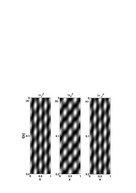
Figure 9: The density distribution of the non-stationary solution (51). The parameters are the same as in Fig.3.

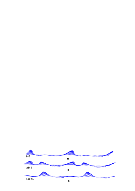
Figure 10: Snapshots of the spin-polarization distributions of the non-stationary solutions (51) at $t=0s,t=0.1s$ and $t=0.2s$, respectively.

III.4 Solution associated to Type D

By applying the spin-rotational transformation to the stationary solution (29), we obtain the the non-stationary solution as follows:

$$\Psi^{\prime}(x,t)=\left(\begin{array}[]{c}\psi_{1}e^{-i(\mu+\mu_{1})t}e^{-i(\alpha+\gamma)}\cos^{2}(\frac{\beta}{2})+\psi_{-1}e^{-i(\mu-\mu_{1})t}e^{-i(\alpha-\gamma)}\sin^{2}(\frac{\beta}{2})\\ \psi_{1}e^{-i(\mu+\mu_{1})t}e^{-i\gamma}\sin\beta/\sqrt{2}-\psi_{-1}e^{-i(\mu-\mu_{1})t}e^{i\gamma}\sin\beta/\sqrt{2}\\ \psi_{1}e^{-i(\mu+\mu_{1})t}e^{i(\alpha-\gamma)}\sin^{2}(\frac{\beta}{2})+\psi_{-1}e^{-i(\mu-\mu_{1})t}e^{i(\alpha+\gamma)}\cos^{2}(\frac{\beta}{2})\\ \end{array}\right),$$ (56)

where $\psi_{1}=\sqrt{A+B\textrm{dn}^{2}(kx,m)}e^{i\theta(x)}$ and $\psi_{-1}=D\textrm{sn}(kx,m)$. The density of each component $n_{i}(x,t)=|\psi_{i}^{\prime}(x,t)|^{2}$, $(i=1,2,3)$ is given by

$$n_{1}(x,t) = |\psi_{1}|^{2}(\cos^{2}\frac{\beta}{2})^{2}+|\psi_{-1}|^{2}(\sin^{2}\frac{\beta}{2})^{2}+2\sqrt{A+B\textrm{dn}^{2}}D\textrm{sn}\sin^{2}\frac{\beta}{2}\cos^{2}\frac{\beta}{2}\cos(2\mu_{1}t-2\gamma+\theta),$$

$$n_{0}(x,t) = |\psi_{1}|^{2}\sin^{2}\beta/2+|\psi_{-1}|^{2}\sin^{2}\beta/2-\sqrt{A+B\textrm{dn}^{2}}D\textrm{sn}\sin^{2}\beta\cos(2\mu_{1}t-2\gamma+\theta),$$

$$n_{-1}(x,t) = |\psi_{1}|^{2}(\sin^{2}\frac{\beta}{2})^{2}+|\psi_{-1}|^{2}(\cos^{2}\frac{\beta}{2})^{2}+2\sqrt{A+B\textrm{dn}^{2}}D\textrm{sn}\sin^{2}\frac{\beta}{2}\cos^{2}\frac{\beta}{2}\cos(2\mu_{1}t-2\gamma+\theta).$$

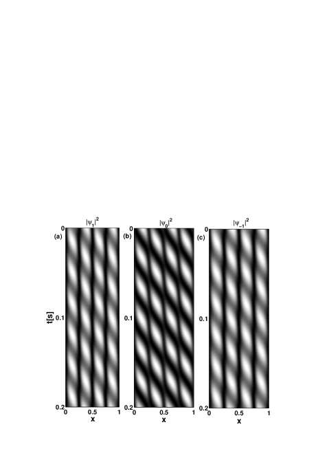
Figure 11: The density distribution of the non-stationary solution (56). The parameters are the same as in Fig.4.

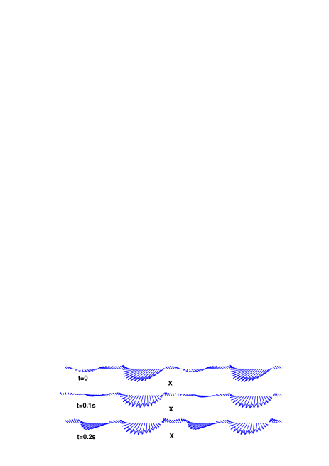
Figure 12: Snapshots of the spin-polarization distributions of the non-stationary solutions (56) at $t=0s,t=0.1s$ and $t=0.2s$, respectively.

Fig.(9) and Fig.(11) depict the temporal evolution of the density in each component from the non-stationary solutions (51) and (56), respectively. They exhibit periodical structures in both the time and the space. Fig.(10) and Fig.(12) describe the evolution of the spin-polarizations for the non-stationary solutions (41) and (46) at $t=0,t=0.1s$ and $t=0.2s$, respectively.

IV Summary

In summary, we have analytically presented several types of stationary solutions to the 1D coupled nonlinear GPEs. Obviously, we can obtain a lot of other stationary solutions with different combination of the Jacobian elliptic functions. In the meanwhile, we derived exact time-evolution solutions by making use of the spin-rotational symmetry of the Hamiltonian. We emphasis that the solutions in Sec.II are stationary. They become non-stationary in Sec.III only after the $SO(3)$ spin-rotation applying to the equations of motion (2). The non-zero parameter $\mu_{1}$ plays an important role in constructing these non-stationary solutions. Our method is applicable to the $F=2$ spinor BECs. Works in this direction are in progress.

This work is supported by the funds from the Ministry of Science and Technology of China under Grant Nos. 2012CB821403 and by the National Natural Science Foundation of China under grant No. 10874018.

References

- (1) M. D. Barrett, J. A. Sauer, and M. S. Chapman, Phys. Rev. Lett. 87, 010404 (2001).
- (2) A. Görlitz, T. L. Gustavson, A. E. Leanhardt, R. Löw, A. P. Chikkatur, S. Gupta, S. Inouye, D. E. Pritchard, and W. Ketterle, Phys. Rev. Lett. 90, 090401 (2003).
- (3) A. E. Leanhardt, Y. Shin, D. Kielpinski, D. E. Pritchard, and W. Ketterle, Phys. Rev. Lett. 90, 140403 (2003).
- (4) J. Stenger, S. inouye, D. M. Stamper-Kurn, H. J. Miesner, and A. P. Chikkatur, Nature 396, 345 (1998).
- (5) H. J. Miesner, D. M. Stamper-Kurn, J. Stenger, S. Inouye, A. P. Chikkatur, and W. Ketterle, Phys. Rev. Lett. 82, 2228 (1999).
- (6) M. Kobayashi, Y. Kawaguchi, M. Nitta, and M. Ueda, Phys. Rev. Lett. 103, 115301 (2009).
- (7) M. Ueda and Y. Kawaguchia, arXiv: 1001.2072 (unpublished).
- (8) Y. Kawaguchi, H. Saito, and M. Ueda, Phys. Rev. Lett. 96, 080405 (2006).
- (9) T.-L. Ho, Phys. Rev. Lett. 81, 742 (1998).
- (10) M.-S. Chang, C. D. Hamley, M. D. Barrett, J. A. Sauer, K. M. Fortier, W. Zhang, L. You, and M. S. Chapman, Phys. Rev. Lett. 92, 140403 (2004).
- (11) K. Murata, H. Saito, and M. Ueda, Phys. Rev. A 75, 013607 (2007).
- (12) A. Imambekov, M. Lukin, and E. Demler, Phys. Rev. A 68, 063602 (2003).
- (13) E. P. Gross, Phys. Rev. 106, 161 (1957).
- (14) V. L. Ginzburg and L.P. Pitaevskii, Sov. phys. JETP 7, 858 (1958).
- (15) F. Dalfovo, S. Giorgini, L. P. Pitaevskii, and S. Stringari, Rev. Mod. Phys. 71, 463 (1999).
- (16) S. Coen and M. Haelterman, Phys. Rev. Lett. 87, 140401 (2001).
- (17) N. Z. Petrović, N. B. Aleksic, A. A. Bastami, and M. R. Belic, Phys. Rev. E. 83, 036609 (2011).
- (18) L. Li, Z. Li, B. A. Malomed, D. Mihalache, and W. M. Liu, Phys. Rev. A 72,033611 (2005).
- (19) W. Zhang, Ö. E. Müstecaplioǧlu, and L. You, Phys. Rev. A 75, 043601 (2007).
- (20) H. E. Nistazakis, D. J. Frantzeskakis, P. G. Kevrekidis, B. A. Malomed and R. Carretero-González, Phys. Rev. A 77,033612(2008).
- (21) C. S. Gardner, J. M. Greene, M. D. Kruskal, and R. M. Miura, Phys. Rev. Lett. 19, 1095 (1967).
- (22) A. R. Sedawy, Appl. Math. Lett. 23, 142 (1973).
- (23) M. Uchiyama, J. Ieda and M. Wadati, J. phys. Soc. Jpn. 75, 064002 (2006).
- (24) J. Ieda, T. Miyakawa, and M. Wadati, Phys. Rev. Lett. 93, 194102 (2004).
- (25) J. Belmonte-Beitia, V. M. Pérez-García, V. Vekslerchik, and P. J. Torres, Phys. Rev. Lett. 98, 064102 (2007).
- (26) G. Theocharis, P. Schmelcher, P. G. Kevrekidis, and D. J. Frantzeskakis, Phys. Rev. A 72, 033614 (2005).
- (27) A. T. Avelar, D. Bazeia, and W. B. Cardoso, Phys. Rev. E 79, 025602(R) (2009).
- (28) D.-S. Wang, X.-H. Hu, and W. M. Liu, Phys. Rev. A 82, 023612 (2010).
- (29) L. D. Carr, C. W. Clark, and W. P. Reinhardt, Phys. Rev. A. 62, 063610 (2000).
- (30) R. M. Bradley, B. Deconinck, and J. N. Kutz, J. Phys. A: Math. Gen. 38, 1901 (2005).
- (31) L. Li, B. A. Malomed, D. Mihalache and W. M. Liu, Phys. Rev. E 73, 066610 (2006).
- (32) D. Yan, J. J. Chang, C. Hamner, P. G. Kevrekidis, P. Engels, V. Achilleos, D. J. Frantzeskakis, R. Carretero-Gonzalez, and P. Schmelcher, Phys. Rew. A 84, 053630 (2011).