Two-Phase ICM in the Central Region of the Rich Cluster of Galaxies Abell 1795: A Joint Chandra, XMM-Newton, and Suzaku View
Abstract
Based on a detailed analysis of the high-quality Chandra, XMM-Newton, and Suzaku data of the X-ray bright cluster of galaxies Abell 1795, we report clear evidence for a two-phase intracluster medium (ICM) structure, which consists of a cool (with a temperature keV) and a hot ( keV) component that coexist and dominate the X-ray emission at least in the central 80 kpc. A third weak emission component ( keV) is also detected within the innermost 144 kpc and is ascribed to a portion of inter-stellar medium (ISM) of the cD galaxy. Deprojected spectral analysis reveals flat radial temperature distributions for both the hot phase and cool phase components. These results are consistent with the ASCA measurements reported in Xu et al. (1998), and resemble the previous findings for the Centaurus cluster (e.g., Takahashi et al. 2009). By analyzing the emission measure ratio and gas metal abundance maps created from the Chandra data, we find that the cool phase component is more metal-enriched than the hot phase one in kpc region, which agrees with that found in M87 (Simionescu et al. 2008). The coexistence of the cool phase and hot phase ICM cannot be realized by bubble uplifting from active galactic nuclei (AGN) alone. Instead, the two-phase ICM properties are better reconciled with a cD corona model (Makishima et al. 2001). In this model, the cool phase may be ascribed to the plasmas confined in magnetic loops, which are surrounded by the intruding hot phase ICM and have been polluted by metals synthesized in the cD galaxy. AGN feedback energy released in the innermost 10 kpc can serve as the heating source to prevent the loop-interior gas from cooling down to temperatures much lower than the observed value. The total gravitating mass profile exhibits a hierarchical structure, regardless of the ICM temperature modeling.
1 INTRODUCTION
First revealed by the Einstein observatory, the spectroscopic temperature of the intracluster medium (ICM) in many cD clusters of galaxies decreases toward the center by a factor of (e.g., Canizares et al. 1988; Mushotzky & Szymkowiak 1988; see also Fabian 1994 for a review). Generally, the appearance of such a central cool component (hereafter CCC) has been described in two possible but competing ways. One is a single-phase (hereafter 1P) scenario, in which a mono-nature plasma showing an inward temperature decrease is assumed to permeate the whole cluster (e.g., Allen et al. 2001; Vikhlinin et al. 2006). The other is a two-phase (hereafter 2P) scenario, in which the cluster’s central region is assumed to be occupied by a mixture of two gas components characterized by discrete temperatures (i.e., hot and cool), of which the relative volume filling factors slowly vary with radius (e.g., Fukazawa et al. 1994, 1998; Takahashi et al. 2009; see Makishima et al. 2001 for a review). Although in many cases it is difficult to distinguish between the 1P and 2P models due to insufficient data quality, the implications of these models on the formation and evolution of the CCC are intrinsically different. In the 1P scenario the CCC is simply interpreted as the dense cluster core, where radiative losses have significantly lowered the gas temperature (see, e.g., Peterson & Fabian 2006 for a review), while the 2P scenario favors an interpretation that the CCC is caused by the cD galaxy, rather than being a cooling portion of the ICM (Makishima et al. 2001 and references therein). Furthermore, the choice between the two scenarios has considerable impact on the accuracies of the measurements of both gas metallicities (e.g., the “Fe-bias” discussed in Buote 2000) and, in some extreme cases, gravitating mass distributions in clusters. For the latter one, the systematic mass bias induced by different ICM models can reach % for the cluster’s central region, which is comparable to the typical deviation between the results obtained in X-ray and lensing studies (e.g., Nagai et al. 2007; Mahdavi et al. 2008). Hence, it is of fundamental and urgent importance to determine which of the two scenarios is valid, based on the analysis of existing high quality X-ray data of nearby, bright clusters.
So far, only a few works have been done to examine the preference between the 1P and 2P ICM models of cD groups and clusters. Of these, Fukazawa et al. (1994) and Ikebe et al. (1999) used the ASCA data to show that a 2P model with temperatures of 1.4 keV and 4.4 keV for the two components is required to describe the CCC of the Centaurus cluster. Their results were recently confirmed by the analysis of the high quality data acquired with the European Photon Imaging Camera (EPIC) and Reflection Grating Spectrometer (RGS) onboard XMM-Newton (Takahashi et al. 2009). The preference for the 2P scenario was also reported in the works on the Fornax cluster (Ikebe et al. 1996; Matsushita et al. 2007) and the NGC 5044 group (Buote & Fabian 1998; Buote et al. 2003; Tamura et al. 2003) with ASCA, Chandra, XMM-Newton, and Suzaku observations. However, due to the lack of such studies on more representative relaxed clusters or groups that exhibit strong CCCs, it is not yet clear whether or not the 2P scenario do surpass the 1P scenario in general, and if yes, to what extent the 2P model can be applied to constrain the origin of the CCC.
To address these issues, we study in this work the rich, bright cD cluster of galaxies Abell 1795 (A1795 hereafter), by jointly analyzing the archival Chandra, XMM-Newton, and Suzaku data. A1795 is suited to our purpose as it is a relaxed, nearby (at a redshift of z ) cluster of galaxies with a luminous X-ray emission (with a keV luminosity of ergs ; Xu et al. 1998), which is found peaked at the giant cD galaxy PGC 049005 (Jones & Forman 1984; Briel & Henry 1996). Under the 2P assumption, Xu et al. (1998) resolved a cool ( keV) and a hot ( keV) component in the central 220 kpc region of this cluster with ASCA, although Ettori et al. (2002) employed the 1P model instead to fit Chandra spectra extracted from the same region, and found an inward temperature decrease to keV. In the past 11 years, X-ray observations of this cluster have been accumulated to ks, 140 ks, and 270 ks with Chandra, XMM-Newton, and Suzaku, respectively. Clearly this is an ideal target for utilizing as much of existing high-quality X-ray data as possible to judge which spectral model is more correct.
The layout of this paper is as follows. Section 2 gives a brief description of our data reduction procedure. The data analysis and results are described in §3. We discuss the physical implication of our analysis in §4, and summarize our work in §5. Throughout the paper we assume a Hubble constant of km s-1 Mpc-1, a flat universe with the cosmological parameters of and , and quote errors by the 90% confidence level unless stated otherwise. At the redshift of this cluster, 1′ corresponds to about 72 kpc. To compare with previous results, we adopt the solar abundance standards of Anders & Grevesse (1989).
2 OBSERVATION AND DATA REDUCTION
2.1 X-ray Observation
2.1.1 Chandra
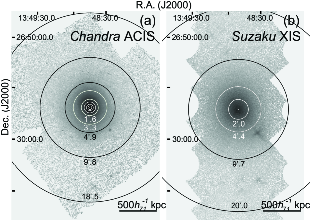
In Table 1, we list 11 Chandra datasets of A1795 obtained with the advanced CCD imaging spectrometer (ACIS), which are all used in the analysis. Among the 11 observations, five ACIS-S3 exposures focused on the cluster center, and six ACIS-I exposures covered off-center regions up to Mpc. All data were telemetered in VFAINT mode, except for the one with ObsID 494 in FAINT mode. Using CIAO v4.4 and CALDB v4.4.7, we removed bad pixels and columns, as well as events with ASCA grades 1, 5, and 7. We then executed the gain, CTI, and astrometry corrections. The cumulative exposure time was reduced from ks to ks after removing intervals contaminated by occasional background flares with count rate % of mean value, which were detected by examining keV lightcurves extracted from source free regions near the CCD edges (e.g., Gu et al. 2009). When available, ACIS-S1 data were also used to crosscheck the determination of the contaminated intervals. The obtained clean exposure time for each observation is listed in Table 1. In Figure 1a we show the combined ACIS image, which has been corrected for exposure but not for background.
2.1.2 XMM-Newton
XMM-Newton was used to observe the central and the south periphery regions of A1795 on 2000 June 26 and 2003 January 13, respectively, both with the EPIC operated in the full window mode with thin filter, and with the RGS in the spectroscopy mode (Table 1). Data reduction and calibration were carried out with SAS v11.0.1. In the screening process we set , and kept events with 0–12 for MOS cameras and events with 0–4 for pn camera. By examining lightcurves extracted in keV and keV from source free regions, we rejected time intervals affected by hard- and soft-band flares, respectively, in which the count rate exceeds a 2 limit above the quiescent mean value (e.g., Katayama et al. 2004; Nevalainen et al. 2005). The cleaned MOS1, MOS2, and pn datasets of the central pointing have exposure times of 43.6 ks, 40.3 ks, and 30.2 ks, respectively (Table 1). The RGS data were screened using the method described in Tamura et al. (2001).
2.1.3 Suzaku
As listed in Table 1, A1795 was also observed by Suzaku on 2005 December 10, with five pointings aimed at its central region, near south and north regions (offset ), and far south and north regions (offset ). The onboard X-ray Imaging Spectrometer (XIS; Koyama et al. 2007) and the Hard X-ray Detector (HXD; Takahashi et al. 2007) were both operated in normal modes. The same XIS datasets were already utilized by Bautz et al. (2009). In analyzing the obtained data, we used the software HEASoft 6.11.1 and latest CALDB (20111109 for the XIS and 20110913 for the HXD). We started with version 2.0 processing data, and removed the data obtained either near South Atlantic Anomaly or at low elevation angles from the Earth rim ( and for night and day, respectively). Cut-off rigidity criteria of GV for HXD-PIN data were also applied. For the XIS instrument, we further examined keV lightcurves of a source free region in each CCD, and filtered off anomalous time bins with count rate above the 2 limit of the quiescent mean value. The combined XIS image is shown in Figure 1b. The data obtained in the far north field are contaminated seriously by solar wind charge exchange emission (Fujimoto et al. 2007), and thus are not included in the following data analysis. The obtained clean exposure times are listed in Table 1. We do not consider HXD-GSO data in this paper.
2.2 Point Sources, Background, and Systematic Uncertainties
We excluded point sources detected beyond a threshold on the ACIS images with the CIAO tool celldetect, and masked the corresponding regions on the EPIC and XIS images after considering the differences in the Point Spread Functions (PSFs) of the instruments. The mask regions have radii of and for the EPIC and XIS, respectively. The point sources outside the ACIS sky coverage were detected and masked using the EPIC images. The ancillary response files (ARFs) and the redistribution matrix files (RMFs) were calculated with the CIAO tools mkwarf and mkacisrmf for the ACIS, and with the SAS tools arfgen and rmfgen for the EPIC. We calculated the RMFs for the RGS using the SAS tool rgsrmfgen, after blurring the line spread function by convolving the raw RMFs with the surface brightness profile (§3.3.1) extracted from the keV ACIS image along the dispersion direction. As for the XIS, we generated the response files using xissimarfgen (version 2008-04-05) and xisrmfgen (version 2007-05-14). To enhance the precision of the Monte-Carlo simulation carried out by xissimarfgen, we created the initial feed photon list by combining all the exposure-corrected and background-subtracted ACIS-I images. The method to build the response of HXD-PIN is described in §3.4.
We estimated the background as a combination of three independent components, i.e., non X-ray background (NXB), cosmic X-ray background (CXB), and Galactic emission. For all the XIS data, we created the NXB spectra using a dark earth observation database. The CXB and Galactic emission components in the XIS data were estimated by analyzing a spectrum extracted from a region about ′ ( Mpc at the distance of A1795) south of the cluster center, which is covered by the dataset with ObsID = 800012050 (Table 1); a similar background region was used in Bautz et al. (2009). Since this region is outside the virial radius Mpc, where the brightness of cluster emission is expected to be in keV (Roncarelli et al. 2006), lower than the detection limit of the XIS, i.e., (Bautz et al. 2009), the ICM component can be ignored in the background fitting. After subtracting the NXB from the extracted spectrum, we fitted the resulting spectrum with an absorbed power law model (photon index ) describing the CXB, and two unabsorbed optically thin thermal models (abundance = 1 , temperatures = 0.08 keV and 0.2 keV; Snowden et al. 1998) describing the Galactic emission. The keV CXB flux was estimated as , which is consistent with the results of Kushino et al. (2002). The obtained CXB + Galactic background template was applied to all the subsequent XIS spectral analysis assuming the same uniform CXB + Galactic emission distribution over the field of view (e.g., Sato et al. 2008).
In order to achieve an accordant background model for the Chandra ACIS, we utilized the above CXB + Galactic background template and calculated the ACIS NXB spectra in an adaptive way as follows. For all ACIS-I observations, background spectra were extracted from regions ′ ( Mpc) away from the cluster center, where the ICM brightness was measured to be weak but cannot be neglected, on a level of 10% to 40% of the CXB + Galactic components (Bautz et al. 2009). We subtracted the CXB + Galactic components from the extracted spectra, whose brightness was fixed at the XIS result obtained above, and fitted the resulting spectra with an empirical NXB model that consists of a broken power law and five narrow Gaussian lines (e.g., Humphrey & Buote 2006), plus a thermal APEC model for the cluster emission. Since the temperature and metal abundance of this ICM component cannot be well constrained, due to the relatively high NXB level of the ACIS, we fixed them to previous Suzaku results (temperature = 2.5 keV, abundance = 0.1 ) reported in Bautz et al. (2009). In the ′ region, average surface brightness of the ICM component was obtained as in keV, which is about % of the CXB + Galactic components, in rough consistent with Bautz et al. (2009). The ACIS-I NXB model was thus determined. The same procedure was applied to all ACIS-S data, but source free regions on the S1 chip were used as the background regions instead. To crosscheck above background model with the blank sky templates, we applied both backgrounds to the spectral analysis in §3.1.1. By fitting the background-subtracted ACIS spectra extracted from with a single-phase thermal model, we found that the ICM temperatures with the two background models differ by 0.35 keV, which is less than the 1 uncertainties of 0.5 keV. The error caused by background model is much smaller for the inner regions, where the ICM emission contributes to % of the total counts in keV (Table 2).
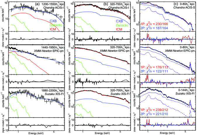
The background model for the XMM-Newton EPIC data was determined with a method similar to that used for the Chandra ACIS data. The EPIC spectra extracted from ′ ( Mpc) away from the cluster center, covered by the data with ObsID = 0109070201, were fit with a model consisting of the CXB + Galactic components, the EPIC NXB model including a broken power law and six Gaussian lines (e.g., Gastaldello et al. 2007; Zhang et al. 2009), and a cluster component approximated by an APEC model. The temperature and abundance of the cluster component were fixed at 2.4 keV and 0.1 (Bautz et al. 2009), respectively, and the keV surface brightness was obtained as (% of the CXB + Galactic components), in agreement with Bautz et al. (2009) and our Chandra estimate. The best-fit CXB + NXB + Galactic models were used to create background spectra. In Figure 2a, we plot the NXB-subtracted background spectra against the best-fit CXB and Galactic components for the ACIS, EPIC, and XIS, as well as the cluster emission component for the former two instruments. For the RGS data, we employed the blank sky template (e.g., Takahashi et al. 2009) in the following spectral analysis.
Errors quoted below in the spectral fittings were estimated by taking into account both statistical and systematic uncertainties. The former was calculated by scanning over the parameter space with the XSPEC command steppar, as the fitting was repeated for a few iterations at each step to ensure that the actual minimum is found. For the latter, we altered the normalization of the CXB spectra by 10% (Kushino et al. 2002) to approximate its field-to-field variation, and similarly, re-normalized the NXB components by 2%, 2%, and 1% for the ACIS, EPIC, and XIS data (e.g., Hickox & Markevitch 2006; De Luca & Molendi 2004; Tawa et al. 2008), respectively, to assess the error ranges. We have also tried assigning a systematic error of 2% to approximate the unassessed calibration uncertainties of the EPIC data (e.g., Takahashi et al. 2009), which turned out to have negligible impacts on the results and thus was not included in the actual fittings.
3 ANALYSIS AND RESULTS
3.1 Azimuthally Averaged Spectral Analysis
3.1.1 Single-phase ICM Model
We extracted the ACIS and EPIC spectra from eight thin annuli, i.e., kpc (), kpc (), kpc (), kpc (), kpc (), kpc (), kpc () and kpc (), and the XIS spectra from four thick annuli, i.e., kpc (), kpc (), kpc () and kpc (). When fitting these spectra, the lower energy cut was set at 0.7 keV, 0.7 keV, and 0.6 keV for the ACIS, EPIC, and XIS, respectively, while the upper cut was fixed at 8.0 keV for all the three detectors. Also, the Si K edge ( keV) was excluded from all the XIS spectra. Independent fittings were carried out for the Chandra (ACIS-S and ACIS-I), XMM-Newton (MOS and pn), and Suzaku (BI and FI) spectrum sets, by applying a common absorbed APEC model and linking all annuli with XSPEC model PROJCT, which performs projection of 3-D shells onto 2-D annuli to evaluate the projected emission of outer shells on inner ones. For each shell, the gas temperature, metal abundance, and column density of the neutral absorber were set free. The best-fit model yielded , 1040/881, and 845/775 for the ACIS, EPIC, and XIS spectra, respectively. Figure 2b and 2c show the best-fit deprojected 1P fittings to the spectra extracted from kpc and core regions ( kpc for the ACIS and EPIC, and kpc for the XIS), respectively.
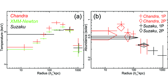
As shown in Figure 3a, the best-fit deprojected 1P temperature drops inwards from keV at kpc to keV in the central 30 kpc, which shows apparent diagnostic of a cool core (e.g., Sanderson et al. 2006). On the other hand, in the cluster’s outskirt ( kpc), the temperature declines outwards steeply down to keV. Generally, our 1P temperature profiles are consistent with previous reports (e.g., Ettori et al. 2002; Vikhlinin et al. 2006; Snowden et al. 2008; Bautz et al. 2009). Incidentally, in kpc, the temperature obtained with the ACIS spectra is by about keV higher than those measured with the EPIC and XIS spectra. This discrepancy can be ascribed to a local temperature structure (see §3.2.2), which is smoothed to some extent in the XMM-Newton and Suzaku data.
Although the best-fit 1P model can reproduce the three data groups with reasonable goodness, i.e., , the fitting residuals become drastically significant in the central 80 kpc regions, where the averaged gas temperature is measured to be keV (Fig. 3a). As shown in Figure 2c, the 1P model significantly underestimates the Fe-L blend and the continuum in 5.0 keV. This indicates that these annular spectra exhibit stronger multi-temperature nature than is predicted by foreground and background contributions from different radii that are accounted for by the PROJCT model. To further examine the issues with the 1P ICM model for these regions, following, e.g., Cavagnolo et al. (2008), we fitted the ACIS spectra in keV and keV with the 1P model, both extracted from the central 80 kpc and corrected for projection effects. The 1P gas temperature obtained in keV ( keV) became lower than its counterpart in keV ( keV) at the 99% confidence level. The bandpass dependence cannot be ascribed to the calibration problem of Chandra at soft band, because a similar dependence can be obtained using the XMM-Newton data, with keV and keV. Thus, the 1P modeling of the ICM is considered inadequate, and a 2P ICM spectral model is hence invoked.
3.1.2 Two-phase ICM Model
Next we investigate whether or not the 2P ICM model, as inferred in the above 1P analysis, is applicable to the spectra extracted in the inner 80 kpc region, after the projection effects are taken into account. Here, the 2P ICM components were both represented by thermal APEC models, which were constrained to have the same metallicity and absorption. Both the cool- and hot-phase ICM temperatures ( and , respectively) were tied among all the thin shells in central 80 kpc, while the 1P ICM model (§3.1.1) was retained for the outer parts. This fitting yielded overall = 1608/1494 and 929/879 for the ACIS and EPIC spectrum sets, respectively. The fitting goodness was compared to the 1P one (§3.1.1) using an F-test, which yielded -statistic of 66.0 and 52.5 for the ACIS and EPIC data, respectively, indicating that the 2P model gives a better fit than the 1P model at 99% confidence level. As shown in Figure 2c, the 2P ICM model apparently better reproduces the Fe-L blend and the continuum in 5.0 keV than its 1P counterpart. This shows that the 2P ICM model is strongly and consistently required for the inner 80 kpc region even after removing (via PROJCT) foreground and background contributions from the outer shells. The 2P temperatures (, ) were determined as (, ) keV and (, ) keV by using the ACIS and EPIC data, respectively. For the regions with kpc, the 2P model does not significantly improve the fitting over the 1P model.
The same 2P ICM model was also applied to the thick shell spectra obtained with the XIS. Compared to the 1P case (§3.1.1; ), the 2P ICM model again gave significantly better fit to the XIS spectra within central kpc region, with reduced chi-squared improved to = 802/773. Since the PSF of the XIS is much wider than those of the ACIS and EPIC, with the XIS alone we cannot constrain the boundary between the 1P and 2P regions to a small radius, as we did with the ACIS and EPIC data. To examine the PSF effect on the spectral fitting of the innermost thick shell ( kpc), we performed a ray tracing simulation (e.g., Ishisaki et al. 2007; Reiprich et al. 2009) based on the ACIS image, and found that the keV counts in this shell are mostly (%) from the emission originated in kpc, only a small fraction (%) come from kpc region where a hotter component ( keV; Figure 3a) is detected with the ACIS data. Hence this hot component cannot bias the 2P result significantly. In fact, the best-fit 2P temperatures for this region, keV and keV, are consistent with those obtained in the thin shell analysis. Thus, the PSF of the XIS little affects the 2P results obtained for the innermost thick shell.
As the most consistent form of our 2P analysis, we simultaneously fitted the thin shell spectra (the ACIS and EPIC) and those from the thick shell (the XIS), by allowing to vary independently the pair of 2P temperatures of each inner shell, i.e., kpc and kpc for the ACIS/EPIC and XIS cases, respectively. Nearly the same fit goodness was achieved (Table 2), and the best-fit and , as shown in Figure 4a and Table 2, exhibit nearly insignificant spatial variations across the inner shells. The values of and are consistent among the three instruments, and broadly consistent with the ASCA result, (, ) = (, ) keV, reported in Xu et al. (1998). In short, the ICM in the cool core of this cluster can be described by two discrete temperatures, keV and keV, which are both consistent with being spatially constant. This makes the simple 2P ICM picture (Makishima et al. 2001) a natural and reasonable description.
3.1.3 A Weak 0.8 keV Spectral Component Within the Central 144 kpc
Employing the 1P formalism, Fabian et al. (2001) reported a filamentary structure in the inner 50 kpc region of A1795, with a possible temperature of keV, apparently lower than the value of obtained in our 2P analysis. To look for such a component, we added a third APEC component to the 2P ICM model describing the XIS data from the central 144 kpc region. Indeed, we obtained a significantly better fit () by adding a third APEC component, whose temperature is keV, while its metal abundance, absorption, and redshift were tied to those of the 2P ICM components. An -test indicates that the probability of this improvement being caused by chance is . The keV luminosity of this 0.8 keV component is ergs , which is consistent with the luminosity of the filamentary structure measured with the ACIS in Fabian et al. (2001; ergs ). As shown in Table 2, the values of and , as well as the ICM abundances, remain nearly the same by adding this 0.8 keV component, because it contributes only % of the total keV luminosity of the central 144 kpc region ( ergs ).
In order to crosscheck the XIS result, we analyzed the XMM-Newton RGS and deprojected EPIC spectra extracted from the central 80 kpc region by fitting them with three component spectral model, i.e., 2P ICM plus a third APEC component. Since the RGS is not so sensitive to hot gas components, we fixed and at the best-fit EPIC results, i.e., 2.0 keV and 5.0 keV, respectively. By fitting the RGS1 and RGS2 spectra simultaneously in Å, a weak 0.8 keV component was again detected, with a probability of for the detection to be caused by chance. The fitting of the EPIC spectra was improved to by including the 0.8 keV component, significantly better than previous 2P fitting in terms of -test (% confidence level). The keV luminosities of this component determined with the RGS and the EPIC are ergs and ergs , respectively, nicely consistent with the XIS value and the ACIS result in Fabian et al. (2001).
3.1.4 Filling Factor of the Cool Phase
Using the high resolution Chandra, XMM-Newton, and Suzaku data, we have demonstrated that the 2P ICM model gives a significantly better description of the ICM thermal condition in the central 80 kpc of A1795 than the 1P counterpart. The cool and hot phase ICM components have keV luminosities of about ergs and ergs , respectively. Also a weak 0.8 keV component has been detected in the same region, which has a keV luminosity of about ergs .
The 2P ICM picture implicitly assumes that these phases with different temperatures coexist, each occupying a certain fraction of the total volume under study in the cluster center, which can be described as volume filling factor (e.g., Ikebe et al. 1999; Makishima et al. 2001; Takahashi et al. 2009). To quantify this quantity, we followed the method described in Ikebe et al. (1999) and calculated the filling factor of the cool phase gas, , where denotes 3-D radius. With , the specific emission measures of the two phases, and , are described as
| (1) |
where and are the density distributions of the cool and hot phases, respectively. Assuming a pressure balance between the two phases
| (2) |
we have
| (3) |
Figure 4b shows radial profiles of , calculated with the best-fit deprojected ACIS, EPIC, and XIS model parameters as listed in Table 2. Thus, the ACIS and EPIC datasets consistently indicate that the hot component dominates in volume over its cool counterpart not only in outer regions, but also in the core region ( kpc). The cool phase gas occupies up to of the volume in the central kpc, whereas declines steeply to below 0.05 outside the central kpc region. The XIS result for the inner kpc is consistent with those of the ACIS and EPIC, whereas the relatively large value of indicated by the outer kpc XIS bin can be attributed to the broad PSF of the XIS. In fact, by performing a ray tracing simulation (see §3.1.2 for more details), the outer XIS bin at kpc was found to be contaminated by photons scattered from the inner regions, in such a way that % of the emission in this region actually comes from the central 144 kpc. In this case, a weighted mean of measured with the XIS over inner kpc and measured with the other two missions at the kpc region becomes , in agreement with the outer XIS point. Hence, after correcting for the PSF effect, all data indicate the same 2P configuration in the central region.
3.1.5 2P vs. Multi-phase ICM Model
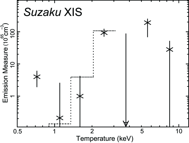
The ICM in the central kpc may alternatively in a multi-phase condition (e.g., Kaastra et al. 2004), to be described by a more complicated emission measure distribution in a wide temperature range than that used in §3.1.2. To examine this possibility, we analyzed the deprojected XIS spectra from the inner 144 kpc region with the same multi-temperature fitting approach as used in Tamura et al. (2001) and Takahashi et al. (2009). That is, the spectra were modeled as a cumulative contribution of seven APEC components, whose temperatures are given as , 1.5, (1.5,…, and (1.5, where is a base temperature and left free in the fitting. The seven components were constrained to have the same metal abundance, and suffer the same absorption. The fit has been acceptable, and the goodness of fitting () is as good as that of the 2P ICM plus a 0.8 keV component model (Table 2). The base temperature was constrained as keV. As shown in Figure 5, in the multi-phase model, only one weak component at keV and two strong components at 2.4 keV and 5.3 keV remain significant (68% confidence level), while the rest components cannot be constrained. This is essentially identical to the 2P ICM plus 0.8 keV modeling. Our result is consistent with the multi-phase fitting with the EPIC data in Kaastra et al. (2004), which also shows a two-temperature structure (2.5 keV and 4.9 keV, see their Table 6) in the cluster center. Hence, the XIS data prefers the discrete 2P model, to a continuous temperature distribution, although the latter cannot be ruled out based on available data.
3.1.6 Metal Abundance and Absorption Distributions
As shown in Figure 3b, the deprojected metal abundance profiles appear roughly consistent between the 1P and 2P ICM modelings (§3.1.1 and §3.1.2, respectively). Both profiles show a peak in the shell of kpc, and a mild decline outwards. This abundance profile, however, should be regarded as an average among those of different elements, because we have so far assumed the solar abundance ratios. To examine the ICM for possible deviation from the solar ratios, we employed two VAPEC models and reran the deprojected 2P fittings of the Suzaku XIS spectra extracted from the central 320 kpc region. Specifically, we left the abundances of O, Mg, Si and Fe free, fixed the abundances of He, C and N at the solar value (Anders & Grevesse 1989), and tied the abundance of Ni to that of Fe and those of other elements (Ne, Al, S, Ar and Ca) to that of Si. This model gave nearly the same set of temperatures for the 2P ICM, and a fit goodness () slightly better than that of the best-fit APEC model (). As shown in Table 3, the best-fit Fe and Si abundances increase significantly towards the center, while the O and Mg abundances are nearly constant throughout the cluster. This confirms the previous ACIS result reported in Ettori et al. (2002; see also Matsushita et al. 2007). We also added another APEC model ( = 0.5 ; see Table 2) in the central 144 kpc to account for the 0.8 keV component, while the model gave nearly the same best-fit abundance profiles for the 2P ICM components.
To examine the possible existence of any intrinsic absorption, we compared the absorption obtained in the spectral analysis with the Galactic value. Regardless of the 1P or 2P modeling, the ACIS and XIS fitting results revealed a significant excess absorption by (Table 3) beyond the Galactic value of , at least in the central 30 kpc region. The excess absorption could not be mitigated by varying the abundances of specific elements (e.g., oxygen) whose emission lines couple with the absorption feature. This result is in good agreement with the ACIS result of Ettori et al. (2002; ). On the contrary, our best-fit EPIC result ( ), as shown in Table 3, implies lack of excess absorption, in agreement with Nevalainen et al. (2007) who used the same XMM-Newton MOS data. The discordance among the three detectors maybe caused by a temporal solar wind charge exchange emission, which biased the EPIC absorption low. As shown in Wargelin et al. (2004), the brightness of charge exchange can reach photon in keV, which is sufficient to undermine the absorption by . The origin of the central excess absorption detected with the ACIS and XIS, on the other hand, still remains unclear.
3.2 Projected 2-D Spectral Analysis
As shown above, the azimuthally-averaged spectral analysis prefers a view of the 2P ICM in the central 80 kpc of A1795 than the 1P counterpart. However, we cannot exclude at present the possibility that the 2P preference is artificially caused by an anisotropic spatial distribution of 1P gas temperature that fluctuates between the range from to . To address this issue, we examine two-dimensional (2-D) temperature distribution in the central region of A1795. Below, 2-D ICM abundance and / distributions are also presented.
3.2.1 Analysis Procedure
Combining five Chandra ACIS-S pointings onto the central region together, we have collected sufficient photons for a high resolution 2-D spectral analysis. Following the procedure described in detail in Gu et al. (2009), a set of discrete points (, ), or “knots”, were chosen in the central kpc, which are randomly distributed with a separation of kpc between any two adjacent knots. To each knot we assigned a circular region, which is centered on the knot and has an adaptive radius of kpc, ensuring that it encloses photons in keV after all detected point sources (§2.2) were excluded. The spectrum extracted from each circular region was fitted with the 1P and 2P APEC models, both subjected to an absorption that was set free. In the 2P spectral fitting, the temperatures of the cool and hot components were fixed at 2.2 keV and 5.7 keV (i.e., best-fit ACIS results; §3.1.2), respectively, and the two components were assumed to have the same abundance and absorption. For each knot , we obtained the best-fit 1P gas temperature, 1P/2P abundance, and specific emission measure ratio between the cool and hot components (/), as well as their errors.
Then, following Gu et al. (2009), we calculated continuous maps based on the obtained knots. For any position within the map region, we defined a scale , so that there are net photons in a circular region centered at , whose radius is . The 1P temperature at was then calculated by a weighted mean of all the knots in the circular region,
| (4) |
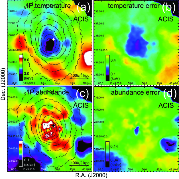
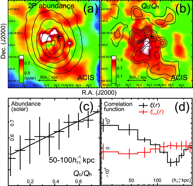
where is the distance from to , and is the Gaussian kernel whose scale parameter is fixed at . The use of compact Gaussian kernel guarantees an angular resolution of kpc within central 100 kpc region. The abundance and / maps, along with their error maps, are calculated in the same way. The resulting 1P temperature and abundance maps are shown in Figure 6, and the 2P abundance (hereafter ) and / maps are presented in Figure 7. The 0.8 keV component (§3.1.3) was not considered in the above 2-D analysis, because it will introduce negligible effects, i.e., uncertainties of about 0.05 keV and 0.02 , to the temperature and abundance measurements, respectively.
3.2.2 Relaxed Cool Core and SE High Temperature Arc
The primary purpose of 2-D spectral analysis is to assess the validity of spherically symmetric temperature distribution that we assumed in the radial 1P/2P analysis. To do this, we examined the obtained 1P temperature map for any significant anisotropic distribution. As shown in Figure 6a, the 1P temperature distribution in the cluster central region exhibits an approximate elliptical symmetry; the temperature variation in the azimuthal direction is about 0.5 keV, 1.0 keV, and 1.0 keV at kpc, kpc, and kpc, respectively, which is insufficient, at least by a factor of three, to imitate the obtained 2P ICM condition. Similar morphology is seen in the / map of the core region as shown in Figure 7b. This confirms that the 2P view is not an artifact caused by a 1P ICM with large azimuthal asymmetry. It also indicates that the two phases, in terms of the 2P view, must be separated on scales smaller than the spatial resolution allowed by the present analysis ( kpc).
The most prominent feature on the 1P temperature map (Fig. 6a) is a high-temperature arc ( keV according to the 1P model) located at kpc southeast (SE) of the cluster’s center, with an open angle of . Given the temperature difference of about 2 keV, the hot structure is significant over the ambient on 90% confidence level. This feature agrees with a high temperature bin ( kpc) on the deprojected ACIS temperature profile shown in Figure 3a. A same high temperature structure was found by Markevitch et al. (2001), who carried out a 1P azimuthal spectral analysis for the southern part of the cluster. Markevitch et al. (2001) also reported a density jump by a factor of near the inner edge ( kpc from the cluster center) of the high-temperature arc, and ascribed the density jump to a cold front. Since both the high-temperature component and the cold front locate outsides of the 2P region (i.e., kpc), they are unable to affect the obtained 2P result significantly, even for the XIS thick shell as indicated by the ray tracing simulation shown in §3.1.2.
3.2.3 A Possible Correlation Between Metal-rich and Cool-phase Gas
A comparison of the map (Fig. 7a) with the / map (Fig. 7b) suggests a spatial correlation on a scale of kpc between the two quantities. Both maps reveal strongly inhomogeneous distributions outside the relaxed core region, with substructures protruding towards southwest, northeast, and northwest of the cluster center by kpc. Most of these substructures show both higher metal abundances, typically by a factor of , and larger cool phase fractions, than their neighborhoods. The best-fit and / values for all the knot-centered circular regions in kpc, obtained in our 2-D spectral analysis (§3.2.1), were compared directly in Figure 7c. Indeed, it reveals a positive linear correlation, which is represented by an analytic form as / . The linear correlation coefficient was obtained as 0.97.
To quantify the suggested correlation, following, e.g., Shibata et al. (2001), we calculated a 2-D cross correlation function as,
| (5) |
where and are averages of and maps, respectively, is the distance between and , and the bracket is ensemble average. The obtained correlation function is shown in Figure 7d. A reference profile () was also calculated, based on a series of random maps, and , which were obtained by randomizing the maps within the same data range and smoothing to the same spatial resolution as the original and maps. The error bars shown in Figure 7d were calculated from the variances of when scattering the and maps by their error maps. Comparing to the , the profile shows a significant excess within 100 kpc, reconfirming the result that cool-phase ICM is indeed more metal-rich.
Given the detected correlation, the assumption made in §3.1.2 and §3.1.6 that the two phases ICM have approximately the same abundances may not stand now. Therefore, we refitted the deprojected XIS spectra of the central kpc region with the 2P ICM (VAPEC + VAPEC) + 0.8 keV component (APEC; 0.5 ) model, same as the one in §3.1.6, except that the iron abundances of the cool and hot phases were let float separately. The absorption column densities of the three components were again tied together in the fitting as a free parameter. We found that the abundance of cool phase ICM () does appear higher than that of the hot one (); i.e., () = (, ) . Compared to the model presented in §3.1.6 (Table 3), the current model improves fit goodness to from , with a probability of for the improvement to be caused by chance.
Following, e.g., Simionescu et al. (2008), the iron abundance to be obtained with a 2P model assuming a single common metallicity can be estimated by
| (6) |
Eliminating and with Eq.(1), we have
| (7) |
Adopting (Fig. 4b) and () obtained above, is then calculated as 0.51, which agrees with that derived with the XIS spectra ( , Table 3). Thus, all the ACIS and XIS results obtained so far can be interpreted as evidence for the relatively high metal abundance of the cool phase ICM.
3.3 Hierarchical Gravitational Potential Structure
3.3.1 Central Excess in X-ray Surface Brightness
In many cool-core clusters, the X-ray surface brightness exhibits an central excess over a model that well fits the outer region. Makishima et al. (2001) argued that the central excess is a combined result of two major effects; the presence of a cool phase component, and the existence of hierarchical potential structure. According to their definition, the hierarchical potential is specified as a halo-in-halo structure, i.e., a smaller potential component is nested on a larger one, so that the overall potential shows a central deepening relative to a simple King profile. Here we examined the surface brightness profile of A1795 for such a central excess. In order to measure the surface brightness profile precisely by taking advantages of both high spatial resolution of the Chandra ACIS and stable low background of the Suzaku XIS, we calculated exposure-corrected surface brightness profiles from the inner 1000 kpc ACIS and kpc XIS data, i.e., and , respectively, where is projected radius. The method described in, e.g., Markevitch et al. (1998), was employed to compensate discrepancies on calibration and instrumental background between the two instruments. First, we performed simulations using the xissim tool (Ishisaki et al. 2007) to smooth the Chandra images with the Suzaku PSF, and extracted the simulated surface brightness profile in the central 1000 kpc, i.e., . Then, was scaled to by solving , where and represent the differences in normalization and NXB, respectively. A modified with the original ACIS resolution was obtained by applying and to in the same way as we normalized .
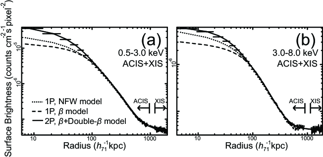
Then, the modified and , shown in Figure 8, were fitted jointly with the model, , where is the central brightness, is the core radius, and is the background. To represent the possible halo-in-halo structure, a double- model was also tested as , where subscripts 1 and 2 denote compact and extended components, respectively. As shown in Table 4, the fit with the model can be rejected on the 95% confidence level, because it significantly underestimates the surface brightness in central kpc, while the double- model gives an acceptable fit to the data. The successful fits in Figure 8 are based on a still more sophisticated model, a +double- gas density model, to be explained later. The properties of the central excess brightness, represented by the compact component (, kpc), are consistent within errors between the keV and keV bands. Such an energy-independent central excess is likely to be caused by an intrinsic hierarchical potential shape, rather than the presence of cool phase component. This result agrees with the earlier ASCA result reported in Xu et al. (1998).
To further quantify the central emission excess, we corrected the surface brightness profile for the projection effect using the best-fit deprojected 2P gas temperature and abundance profiles (Table 2; §3.1.2). The observed surface brightness profile was modeled as
| (8) |
where is the cooling function, and are the same as in Eq.(1), and is the averaged background value. Following Ikebe et al. (1999), we represented the specific emission measure profiles by a 2P +double- model, which consists of a component for the cool phase ICM,
| (9) |
and a double- component for the hot phase ICM,
| (10) |
where , , and are the model normalizations of the cool phase, the compact hot phase, and the extended hot phase components, respectively. The filling factor is renormalized into these parameters.
With these preparations, we fitted the keV ACIS + XIS surface brightness profiles using Eq.(8), where was calculated from the best-fit 2P spectral parameters. The fit has been successful with . The best-fit values of , , , , , and are given in Table 4. The fittings with surface brightness profiles extracted in different energies (i.e., keV and keV bands) are shown in Figure 8. As presented in Table 4, all the fittings yielded consistent parameters for the 2P +double- model.
In some clusters, the central excess can be alternatively explained by a cuspy dark matter distribution proposed in Navarro, Frenk, & White (1996; hereafter NFW model). The NFW model predicts potential structure with a single spatial scale, instead of the dual structure assumed by the +double- model. Given the NFW dark matter density profile,
| (11) |
where is the critical density, is characteristic density, and is scale radius, the ICM density profile is expressed as
| (12) |
where is model normalization and is a parameter related to the ICM temperature. Then the projected ICM surface brightness profile was modeled as a single component,
| (13) |
We found this NFW model cannot give acceptable fits to the keV surface brightness profile for the entire cluster, with a minimum . As shown in Figure 8, the central excess emission is too strong to be explained by the NFW model that best-fits the kpc region. Hence, we reconfirmed the ASCA result reported in Xu et al. (1998) that the halo-in-halo hierarchical model is preferred to the single-halo NFW model in A1795.
3.3.2 Central Excess in Total Gravitating Mass
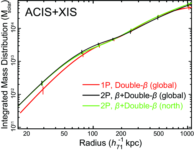
Next we calculated the total gravitating mass profile based on the best-fit 2P temperatures (§3.1.2) and the emission measure profiles obtained with the +double- model (§3.3.1). With the help of Eqs.(1)-(3), the best-fit emission measure profiles, and , were converted to gas density profiles of the cool and hot phases, and , respectively. Then, under the assumptions of spherical symmetry and hydrostatic equilibrium, the gravitating mass profile was calculated as
| (14) |
where = = is the gas pressure, is the averaged gas mass density, is the approximated mean molecular weight, and is the proton mass. As shown in Figure 9, the obtained mass profile exhibits a significant shoulder-like feature at kpc, enclosing an excess mass () of about above a flat core mass distribution calculated with the extended hot phase component alone. Our result agrees with the ASCA result, kpc and , as reported in Xu et al. (1998).
To examine systematic errors of the mass profile due to different modelings of the ICM temperature distribution, we also calculated the gravitating mass profile using the best-fit deprojected 1P spectral parameters (§3.1.1). The projected X-ray surface brightness profile was modeled with a single ICM component as
| (15) |
where the specific emission measure is given by a double- model,
| (16) |
The fit is as good as the 2P case, with . The resulting mass profile, derived by substituting = and to Eq.(14), is shown in Figure 9 by a red curve. Thus, the shoulder-like potential structure is again found, although the 1P model systematically underestimates the gravitating mass within 80 kpc by %. This bias is negligible in kpc.
Another concern is that, the assumption of hydrostatic equilibrium may not hold for the ICM near the cold front located southeast of the cluster center (§3.2.2), casting doubt on the validity of mass profile obtained in the related region (Markevitch et al. 2001). To investigate this, we excluded the southern half of the cluster and recalculated mass profile for the northern half using the best-fit 2P spectral results and surface brightness profile with the ACIS data. The 2P temperatures, keV and keV, are consistent with previous ACIS results. The same is the obtained profile, except for the annulus of the cold front (i.e., kpc), where is lower than by % in kpc. After comparing to in Figure 9, we found that the shoulder-like structure, though diminished by %, still remains significant after the high-temperature arc is excluded. Hence we conclude that the existence of central hierarchical structure is unambiguously confirmed in A1795.
3.4 Hard X-ray Emission Component
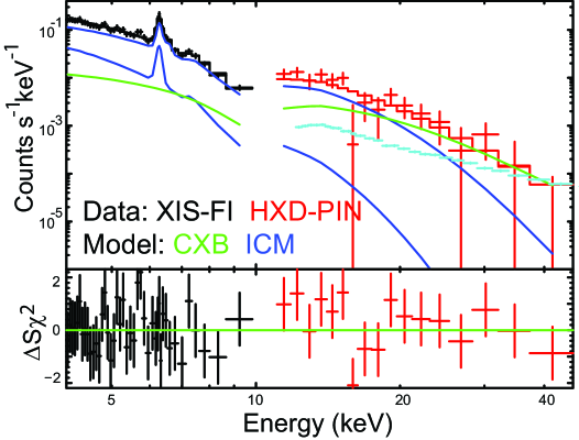
Here we examined the keV HXD-PIN data for possible existence of any extra emission component. First, following, e.g., Nakazawa et al. (2009), we calculated the effective area of the HXD-PIN considering the location and extension of the source. Based on the observed best-fit gas temperature and gas density profiles (Fig. 4a and Table 4), we calculated the ICM surface brightness distribution map in keV. Then we divided the whole HXD field of view into blocks, calculated the point source ARF for each block at using the ftool hxdarfgen, and convolved all the monochromatic ARFs with the normalized . The PIN/XIS cross normalization factor of 1.132 (Suzaku Memo 2007-11111http://www.astro.isas.ac.jp/suzaku/doc/suzakumemo/suzakumemo-2007-11.pdf) was also adopted in the resulting ARF. To assess the NXB level, we utilized the “tuned” NXB model, which provides an optimized reproductivity by making use of HXD-GSO information (Suzaku Memo 2008-03222http://www.astro.isas.ac.jp/suzaku/doc/suzakumemo/suzakumemo-2008-03.pdf). The CXB model was assumed as 1.0 keV 40.0 keV) photons , where the normalization was set to match the HXD-PIN opening angle of 0.32 (e.g., Nakazawa et al. 2009).
As shown in Figure 10, the NXB-subtracted XIS and HXD-PIN spectra in keV were tentatively fitted with a CXB + ICM model. The CXB component was modeled by a cutoff powerlaw with index of 1.29 (Boldt 1987), and the ICM component was represented by the 2P model derived in §3.1.2. The 2P temperatures were set to (, ) = (, ) keV, and their relative normalizations were fixed at the best-fit value in our 2P analysis with the XIS. The fitting is acceptable with , and no additional hard X-ray component is required in keV band. To obtain an upper limit on any hard X-ray component, we fitted the combined XIS-HXD spectra with a 2P ICM plus power-law model (Nakazawa et al. 2009). Taking account of the NXB systematic uncertainty of 2.0% at 90% confidence level (Fukazawa et al. 2009), the upper limit flux of power-law emission in keV band was estimated to be ergs . A similar upper limit on any thermal hard X-ray excess, ergs , was obtained by alternatively fitting the combined spectra with 2P ICM plus a 10 keV APEC model.
4 DISCUSSION
We have analyzed Chandra, XMM-Newton, and Suzaku data of the relaxed galaxy cluster A1795. The deprojected spectra extracted from the central 80 kpc region have been successfully reproduced by invoking two major ICM components with discrete temperatures, indicating a 2P property. A third weak 0.8 keV component is marginally detected in the core region. In §3.2, we analyzed the Chandra data, under 2-D (spatially) and 2P (spectroscopically) formalism. The ICM metallicity was found to show a similar spatial distribution to that of the cool phase component, indicating that the cool phase ICM is more metal-enriched than the hot phase one.
4.1 Two-phase ICM Properties
A joint fitting of the thin shell spectra from the ACIS and EPIC, and thick shell spectra from the XIS, consistently indicates a clear preference of the two-phase ICM nature, over the single-phase one, in the central 80 kpc region of A1795. The ICM therein can be characterized by two representative temperatures, keV and keV for the hot and cool phases, respectively, whose keV luminosities were estimated to be ergs and ergs . Both components show insignificant temperature gradients in the 80 kpc region. The hot phase ICM dominates in volume over the cool phase one by a factor of , even in the innermost region. The 2P view is consistent with previous ASCA results reported in Xu et al. (1998). Employing the 2P ICM model and fitting the cool phase and hot phase components with and double- gas density models, respectively, we quantified the shape of cluster potential. As shown in Figure 9, the total gravitating mass profile exhibits a central mass excess (), which has a similar spatial scale to the region of clear 2P property. This indicates a potential hierarchy, with a 100 kpc level halo nested in the center of a cluster-scale one.
As shown in Figure 3b, the ICM metallicity is also enhanced in the 2P region. Furthermore, by comparing the 2-D metallicity and the emission measure ratio maps created with the 2P ICM model, we found a possible spatial correlation on level between the cool-phase fraction (or ) and the ICM metallicity in the kpc region. The 2-D maps also revealed a filamentary distribution of the cool, metal-rich gas in this region. The subsequent 2P fitting to the XIS spectra confirmed the metallicity enhancement in the cool phase relative to the hot phase, giving the best-fit iron abundances of the cool phase and hot phase ICM to be 0.80 and 0.36 , respectively. Such a picture resembles the previous findings of the metal-rich, multi-phase arms in M87 (Simionescu et al. 2008). In the innermost core of A1795, i.e., kpc, however, a dip is seen in the abundance distribution, which does not correlate with the cool phase fraction. Such a feature is also seen in the coolest spots of some other clusters, while its origin still remains unclear (e.g., Sanders et al. 2006).
In §3.1.3 and §3.1.5, we showed that the XIS and RGS spectra of the central 144 kpc region can be better reproduced by including an additional weak 0.8 keV component, without significantly revising the properties of the cool and hot ICM components. This 0.8 keV component has a keV luminosity of ergs , and is dimmer than the hot ICM component by two orders of magnitude. Since the temperature and luminosity of this component are consistent with those of an X-ray/H filament in the core of A1795 as reported in Fabian et al. (2001), the 0.8 keV emission might be associated with a portion of ISM of the cD galaxy, which is presumably confined within some filamentary magnetic structures.
The 2P formalism has also been successful for the central region of the Centaurus cluster, as firstly reported by Fukazawa et al. (1994) and Ikebe et al. (1999) with ASCA data, and recently reinforced by Takahashi et al. (2009) using XMM-Newton. According to Takahashi et al. (2009), the cool phase and hot phase coexist and dominate in the central 70 kpc of the Centaurus cluster, exhibiting a temperature ratio . These properties are analogous to those of A1795. In addition, a similar central excess in the total gravitating mass profile, with a radius of 50 kpc, has also been found in the Centaurus cluster (Ikebe et al. 1999). Thus, the two clusters are very similar in the ICM properties, as well as in the total mass distribution.
As shown in §3.1.4 and Figure 4b, the cool ( keV) phase component of A1795 occupies up to only 20% volume even in the innermost region, and in Figure 6 and 7, no apparent separation on the spatial distribution is seen between the cool phase and hot phase ICM in the cluster core. This indicates that the cool phase is substantially mixed into the surrounding hot phase, instead of forming any “cool-phase-only” core on scale of kpc. Since such a 2P structure is seen predominately around a cD galaxy, with an enhanced metallicity (particularly in the cool phase), the phenomenon is very likely related to the cD galaxy.
4.2 Bubble Uplifting Model
One possible formation mechanism of the 2P structure could be an AGN-driven gas transport. As indicated by numerical simulations, e.g., Churazov et al. (2001) and Guo & Mathews (2010), the buoyant bubbles created by AGN outbursts can drag a certain amount of surrounding cool, metal-rich gas to larger radii. For example, the ICM in central 30 kpc regions of the Hydra A cluster and M87 are known to be in a 2P or multi-phase form (Ikebe et al. 1997; Molendi 2002). More recently, the distributions of cool phase ICM were found to coincide with the powerful radio lobes and X-ray cavities, hence, the bubble uplifting model has successfully been invoked for both Hydra A cluster and M87 (Nulsen et al. 2002; Simionescu et al. 2008). These properties may be useful to explain the origin of the co-existing 2P ICM. As for A1795, by adopting the obtained distributions of total gravitating mass and cool phase gas mass ( and , respectively; §3.3.2), the energy required to uplift the cool component from cD galaxy center to current position (average kpc) is estimated as ergs, which is consistent with the amount of mechanical energy injected from its central AGN outburst (Rafferty et al. 2006). Nevertheless, the faint X-ray cavity detected in A1795 is located kpc from the center (Birzan et al. 2004), apparently much smaller than the radius of the cool phase ICM as shown in the obtained 2-D temperature and the / maps (Fig. 6 & 7). Hence the appearance of the 2P ICM cannot be solely ascribed to bubble uplifting via recent AGN activity. Neither can the cool phase ICM be bubble remnant, since the uplifted gas would conductively mix and reach thermal equilibrium with the surrounding hot phase ICM quickly, i.e., within yrs (e.g., Simionescu et al. 2008), after the bubble is torn apart.
4.3 cD Corona Model
The most natural and effective way to sustain a stable 2P structure is to separate the two ICM phases by magnetic fields. In such a case, the two phases become thermally insulated with each other, since the gyroradius of a thermal electron in a G field is smaller than its mean free path by about orders of magnitude (Sarazin 1988). Actually, cluster central regions are often threaded by rather strong ( G; Ge & Owen 1993) magnetic fields, which are possibly related to the cD galaxy. Employing a general topological classification of such cD-galaxy-related magnetic field lines into closed and open ones, Makishima et al. (2001) proposed that the closed loops (with their both ends anchored to the cD galaxy) are filled with the cool phase ICM, while the open-line regions, connecting to outer regions, are permeated by the hot phase. Thus, the cool phase component is expected to emerge as numerous filamentary substructures in the core region, while the hot phase distributes throughout the vast cluster volume. In addition, the cool phase is naturally more metal-rich than the hot phase in this scenario, as the supernova yield of the cD galaxy may be largely confined within the loops (Takahashi et al. 2009), which are surrounded by intruding, less contaminated hot phase ICM. This “cD corona” model is expected to provide a natural account for the appearance of metal-rich cool phase ICM in the center of A1795.
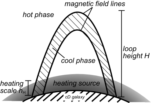
As the cool phase is thermally insulated from the hot phase, and the radiative transport between the two phases can be ignored (Sarazin 1988), a continuous, efficient heating source located in the central region is required to prevent it from collapsing due to radiative cooling (see Aschwanden et al. 2001 for a review). As first pointed out by Rosner, Tucker & Vaiana (1978; hereafter RTV) for solar corona, and applied successfully to the Centaurus cluster by Takahashi et al. (2009), a loop structure as illustrated in Figure 11 has a built-in feedback mechanism to maintain thermal stability for the cool phase plasma. In order to characterize the loop heating mechanism in a quantitative way, we employed an updated version of RTV model, an analytical solution to the hydrostatic model introduced in Aschwanden & Schrijver (2002; AS02 hereafter) for solar corona and applied it to the 2P ICM. This model considers a thin, arch-like loop delineating magnetic field lines, for which the pressure between the loop-interior and surrounding plasmas are in equilibrium. To constrain the temperature and density structures of the loop, AS02 assumed mass and momentum conservations along the loop, as well as a total energy balance involving radiative loss rate, heating rate, and thermal conductive flux. The heating rate function has been defined in form of , where is heating rate at the bottom of loop, is the height in the loop plane, and is the scale height of the heating source (Fig. 11). The analytic solution by AS02 gave a loop temperature distribution increasing with in general, and the exact temperature gradient was predicted to be sensitive to the heating scale . As shown in Figure 9 of AS02, for a uniform heating, i.e., , where is the loop height, the loop temperature exhibits a mild decrease towards the loop bottom by %, while for a small scale heating at the bottom, i.e., , a large part of the loop becomes near isothermal, with only a sharp, small-scale temperature drop seen at the footpoints. Such a loop also obey a scaling law, as defined in Eq.(29) of AS02 (also see Eq.19 below), which describes the loop maximum temperature as a function of , , and external pressure at footpoint . Another important property of the loop-confined plasma is that, as shown in Eq.(30) of AS02, shows rather weak dependence on the heating rate , i.e., , because a decrease (or increase) in will make the loop thinner (or thicker), so as to keep the plasma luminosity nearly equal to .
Specifically, following AS02, the temperature distribution of the loop-interior plasma is expected as
| (17) |
and the density distribution can be calculated as
| (18) |
where
| (19) |
is directly derived from the scaling law (Eq.29 of AS02), is the gravitational acceleration calculated from the obtained total mass profile (§3.3.2), and are the best-fit analytic functions, as defined in Eqs.(20) and (21) of AS02, respectively, to reproduce the dependence of on derived in a numerical way, and similarly, is the best-fit empirical function of scaling law factor given in Eq.(35) of AS02. We adopted the best-fit coefficients of the hydrostatic solutions presented in Table 1 of AS02 to characterize , , and , and then, to calculate , , and based on the loop properties. In short, given a set of (), we may determine the temperature and density distributions of the loop-interior plasma.
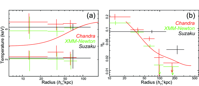
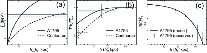
Next we applied the AS02 model to the X-ray observations of A1795 and, for a comparison, the Centaurus cluster, both harboring a prominent cool phase in the central region. In the calculation we determined the external pressures by the temperatures and densities of the hot phases measured at the innermost regions, and took the loop heights kpc and 70 kpc for A1795 and the Centaurus cluster, respectively, as indicated by the radii of cool phases (§3.1.2; Takahashi et al. 2009). Figure 12a shows the predictions of Eq.(19), i.e., as a function of , in comparison with the measured maximum cool phase temperature, i.e., keV and keV for A1795 and the Centaurus cluster (Fig. 4a; Takahashi et al. 2009), respectively. This comparison yields kpc for A1795 and 18 kpc for the Centaurus cluster, which indicates that the heating is concentrated at the bottoms of the loops.
Since the sizes of radio lobes of the central AGNs in A1795 and the Centaurus cluster ( kpc and kpc, respectively; Ge & Owen 1993; Taylor et al. 2002) agree well with estimated above, we speculate that the AGN feedback is a candidate heating source for the coronal loops. The life time of the radio lobes can be estimated by yrs, roughly consistent with the cooling time of the cool phase ICM. Furthermore, as shown in Rafferty et al. (2006), the heating rates provided by the central AGN outbursts in A1795 and the Centaurus cluster were estimated to be ergs and ergs , respectively, which agree well with their cool phase luminosities ( ergs for A1795 and ergs for the Centaurus cluster).
Having obtained the estimates of and for the two clusters, we then calculated, via Eq.(17), the profiles, and show the results in Figure 12b. Thus, a mild inward temperature decrease is expected, especially for the Centaurus cluster. Actually, Takahashi et al. (2009) showed (in their Fig. 4a) that the cool phase temperature of the Centaurus cluster decreases mildly, from keV (as already used in Fig. 12a) at kpc , to keV = 0.72 at kpc. This latter value, when plotted on Figure 12b (with a dashed cross), agrees with the prediction. The same is true in the A1795 case, which shows a more flat profile that is consistent with the measured value of at 15 kpc (solid cross on Fig. 12b). As shown in Figure 12c, we applied the obtained to Eq.(18) and calculated the normalized loop gas density profile for A1795, which again agrees well with the observed profile.
In summary, the cD corona view, combined with the AS02 modeling of the loop-confined plasmas, can account for several important properties of inner regions of A1795 and the Centaurus cluster. These properties include the stable 2P structure, the higher metallicity of the cool phase, the absolute values of , and the spatial and density distributions.
5 CONCLUSION
By analyzing the Chandra, XMM-Newton, and Suzaku data of the X-ray bright galaxy cluster A1795, we report clear preference for the 2P ICM model in the central 80 kpc, which consists of a cool phase ( keV) and a hot phase ( keV) component. This 2P model provides significantly better fit to the deprojected spectra than the 1P model with continuous temperature profile, while the latter cannot be fully ruled out based on current data. Combining the Suzaku XIS and the XMM-Newton EPIC & RGS, we have marginally detected a third weak 0.8 keV component in the inner 144 kpc region that can be ascribed to a portion of ISM component of the cD galaxy. Based on a 2-D spectral analysis with the ACIS data, we have revealed a possible spatial correlation between the cool phase and metal-rich gas in the kpc region. A follow-up XIS analysis shows consistent result, that the cool phase ICM does exhibit a higher metallicity ( ) than the hot phase one ( ). Hence, we have successfully resolved a 2 keV, metal-rich component associated with the cD galaxy, which is spatially mixed but thermally separated with the surrounding 5 keV cluster component. All these properties can be explained by the cD corona model incorporating with the AS02 solution for quiescent coronal loops.
Acknowledgments
This work was supported by the Grant-in-Aid for Scientific Research (S), No. 18104004, titled ”Study of Interactions between Galaxies and Intra-Cluster Plasmas”, and by the National Science Foundation of China (Grant No. 10878001 and 10973010, and National Science Fund for Distinguished Young Scholars) and the Ministry of Science and Technology of China (Grant No. 2009CB824900 and 2009CB824904). L. G. was supported by the Grand-in-Aid for JSPS fellows, through the JSPS Postdoctoral Fellowship program for Foreign Researchers.
References
- (1) Allen, S. W., Schmidt, R. W., & Fabian, A. C. 2001, MNRAS, 328, L37
- (2) Anders, E., & Grevesse, N. 1989, Geochim. Cosmochim. Acta, 53, 197
- (3) Aschwanden, M. J., Poland, A. I., & Rabin, D. M. 2001, ARA&A, 39, 175
- (4) Aschwanden, M. J., & Schrijver, C. J. 2002, ApJS, 142, 269 (AS02)
- (5) Bautz, M. W., Miller, E. D., Sanders, J. S., Arnaud, K. A., Mushotzky, R. F., Porter, F. S., Hayashida, K., Henry, J. P., Hughes, J. P., Kawaharada, M., Makishima, K., Sato, M., & Tamura, T. 2009, PASJ, in press [preprint arXiv:0906.3515]
- (6) Birzan, L., Rafferty, D. A., McNamara, B. R., Wise, M. W., & Nulsen, P. E. J. 2004, ApJ, 607, 800
- (7) Boldt, E. 1987, Phys. Rep., 146, 215
- (8)
- (9) Briel, U. G., & Henry, J. P. 1996, ApJ, 472, 131
- (10)
- (11) Buote, D. A. 2000, MNRAS, 311, 176
- (12)
- (13) Buote, D. A., & Fabian, A. C. 1998, MNRAS, 296, 977
- (14)
- (15) Buote, D. A., Lewis, A. D., Brighenti, F., & Mathews, W. G. 2003, ApJ, 594, 741
- (16)
- (17) Canizares, C. R., Markert, T. H., & Donahue, M. E. 1988, in , ed. A. C. Fabian (Dordrecht: Kluwer), p. 63
- (18) Cavagnolo, K. W., Donahue, M., Voit, G. M., & Sun, M. 2008, ApJ, 682, 821
- (19)
- (20) Churazov, E., Brggen, M., Kaiser, C. R., Bhringer, H., & Forman, W. 2001, ApJ, 554, 261
- (21) De Luca, A., & Molendi, S. 2004, A&A, 419, 837
- (22) Ettori, S., Fabian, A. C., Allen, S. W., & Johnstone, R. M. 2002, MNRAS, 331, 635
- (23)
- (24)
- (25) Fabian, A. C. 1994, ARA&A, 32, 277
- (26) Fabian, A. C., Sanders, J. S., Ettori, S., Taylor, G. B., Allen, S. W., Crawford, C. S., Iwasawa, K., & Johnstone, R. M. 2001, MNRAS, 321, L33
- (27) Fujimoto, R., Mitsuda, K., Mccammon, D., Takei, Y., Bauer, M., Ishisaki, Y., Porter, S. F., Yamaguchi, H., Hayashida, K., & Yamasaki, N. Y. 2007, PASJ, 59, 133
- (28) Fukazawa, Y., Ohashi, T., Fabian, A. C., Canizares, C. R., Ikebe, Y., Makishima, K., Mushotzky, R. F., & Yamashita, K. 1994, PASJ, 46, L55
- (29) Fukazawa, Y., Makishima, K., Tamura, T., Ezawa, H., Xu, H., Ikebe, Y., Kikuchi, K., & Ohashi, T. 1998, PASJ, 50, 187
- (30) Fukazawa, Y., et al. 2009, PASJ, 61, 17
- (31) Gastaldello, F., Buote, D. A., Humphrey, P. J., Zappacosta, L., Bullock, J. S., Brighenti, F., & Mathews, W. G. 2007, ApJ, 669, 158
- (32) Ge, J. P., & Owen, F. N. 1993, AJ, 105, 778
- (33) Gu, L., Xu, H., Gu, J., Wang, Y., Zhang, Z., Wang, J., Qin, Z., Cui, H., & Wu, X.-P. 2009, ApJ, 700, 1161
- (34) Guo, F., & Mathews, W. G. 2010, ApJ, 717, 937
- (35) Hickox, R. C., & Markevitch, M. 2006, ApJ, 645, 95
- (36) Humphrey, P. J., & Buote, D. A. 2006, ApJ, 639, 136
- (37)
- (38) Ikebe, Y., Ezawa, H., Fukazawa, Y., Hirayama, M., Ishisaki, Y., Kikuchi, K., Kubo, H., Makishima, K., Matsushita, K., Ohashi, T., Takahashi, T., & Tamura, T. 1996, Nature, 379, 427
- (39)
- (40) Ikebe, Y., Makishima, K., Ezawa, H., Fukazawa, Y., Hirayama, M., Honda, H., Ishisaki, Y., Kikuchi, K., Kubo, H., Murakami, T., Ohashi, T., Takahashi, T., & Yamashita, K. 1997, ApJ, 481, 660
- (41)
- (42) Ikebe, Y., Makishima, K., Fukazawa, Y., Tamura, T., Xu, H., Ohashi, T., & Matsushita, K. 1999, ApJ, 525, 58
- (43) Ishisaki, Y., et al. 2007, PASJ, 59, 113
- (44)
- (45) Jetha, N. N., Ponman, T. J., Hardcastle, M. J., & Croston, J. H. 2007, MNRAS, 376, 193
- (46)
- (47) Jones, C., & Forman, W. 1984, ApJ, 276, 38
- (48)
- (49) Kaastra, J. S., Tamura, T., Peterson, J. R., Bleeker, J. A. M., Ferrigno, C., Kahn, S. M., Paerels, F. B. S., Piffaretti, R., Branduardi-Raymont, G., & Bhringer, H. 2004, A&A, 413, 415
- (50)
- (51) Katayama, H., Takahashi, I., Ikebe, Y., Matsushita, K., & Freyberg, M. J. 2004, A&A, 414, 767
- (52)
- (53) Koyama, K., et al. 2007, PASJ, 59, 23
- (54) Kushino, A., Ishisaki, Y., Morita, U., Yamasaki, N. Y., Ishida, M., Ohashi, T., & Ueda, Y. 2002, PASJ, 54, 327
- (55)
- (56) Mahdavi, A., Hoekstra, H., Babul, A., & Henry, J. P. 2008, MNRAS, 384, 1567
- (57) Makishima, K., Ezawa, H., Fukuzawa, Y., Honda, H., Ikebe, Y., Kamae, T., Kikuchi, K., Matsushita, K., Nakazawa, K., Ohashi, T., Takahashi, T., Tamura, T., & Xu, H. 2001, PASJ, 53, 401
- (58)
- (59) Markevitch, M., Forman, W. R., Sarazin, C. L., & Vikhlinin, A. 1998, ApJ, 503, 77
- (60)
- (61) Markevitch, M., Vikhlinin, A., & Mazzotta, P. 2001, ApJ, 562, L153
- (62)
- (63) Matsushita, K., Bhringer, H., Takahashi, I., & Ikebe, Y. 2007, A&A, 462, 953
- (64)
- (65) Molendi, S. 2002, ApJ, 580, 815
- (66) Mushotzky, R. F., & Szymkowiak, A. E. 1988, in , ed. A. C. Fabian (Dordrecht: Kluwer), p. 53
- (67) Nagai, D., Vikhlinin, A., & Kravtsov, A. V. 2007, ApJ, 655, 98
- (68)
- (69) Nakazawa, K., Sarazin, C. L., Kawaharada, M., Kitaguchi, T., Okuyama, S., Makishima, K., Kawano, N., Fukazawa, Y., Inoue, S., Takizawak, M., Wik, D. R., Finoguenov, A., & Clarke, T. E. 2009, PASJ, 61, 339
- (70) Navarro, J. F., Frenk, C. S., & White, S. D. M. 1996, ApJ, 462, 563
- (71) Nevalainen, J., Markevitch, M., & Lumb, D. 2005, ApJ, 629, 172
- (72) Nevalainen, J., Bonamente, M., & Kaastra, J. 2007, ApJ, 656, 733
- (73)
- (74) Nulsen, P. E. J., David, L. P., McNamara, B. R., Jones, C., Forman, W. R., & Wise, M. 2002, ApJ, 568, 163
- (75)
- (76) Peterson, J. R., & Fabian, A. C. 2006, Phys. Rep., 427, 1
- (77)
- (78) Rafferty, D. A., McNamara, B. R., Nulsen, P. E. J., & Wise, M. W. 2006, ApJ, 652, 216
- (79) Reiprich, T. H., Hudson, D. S., Zhang, Y.-Y., Sato, K., Ishisaki, Y., Hoshino, A., Ohashi, T., Ota, N., & Fujita, Y. 2009, A&A, 501, 899
- (80) Roncarelli, M., Ettori, S., Dolag, K., Moscardini, L., Borgani, S., & Murante, G. 2006, MNRAS, 373, 1339
- (81) Rosner, R., Tucker, W. H., & Vaiana, G. S. 1978, ApJ, 220, 643
- (82) Sanders, J. S., & Fabian, A. C. 2006, MNRAS, 370, 63
- (83) Sanderson, A. J. R., Ponman, T. J., & O’Sullivan, E. 2006, MNRAS, 372, 1496
- (84) Sarazin, C. J. 1988, - (Cambridge University Press)
- (85)
- (86) Sato, K., Matsushita, K., Ishisaki, Y., Yamasaki, N. Y., Ishida, M., Sasaki, S., & Ohashi, T. 2008, PASJ, 60, 333
- (87)
- (88) Simionescu, A., Werner, N., Finoguenov, A., Bhringer, H., & Brggen, M. 2008, A&A, 482, 97
- (89) Shibata, R., Matsushita, K., Yamasaki, N. Y., Ohashi, T., Ishida, M., Kikuchi, K., Bhringer, H., & Matsumoto, H. 2001, ApJ, 549, 228
- (90) Snowden, S. L., Egger, R., Finkbeiner, D., Freyberg, M. J., & Plucinsky, P. P. 1998, ApJ, 493, 715
- (91) Snowden, S. L., Mushotzky, R. F., Kuntz, K. D., & Davis, D. S. 2008, A&A, 478, 615
- (92)
- (93)
- (94) Takahashi, I., Kawaharada, M., Makishima, K., Matsushita, K., Fukazawa, Y., Ikebe, Y., Kitaguchi, T., Kokubun, M., Nakazawa, K., Okuyama, S., Ota, N., & Tamura, T. 2009, ApJ, 701, 377
- (95) Takahashi, T., et al. 2007, PASJ, 59, 35
- (96)
- (97) Tamura, T., Kaastra, J. S., Peterson, J. R., Paerels, F. B. S., Mittaz, J. P. D., Trudolyubov, S. P., Stewart, G., Fabian, A. C., Mushotzky, R. F., Lumb, D. H., & Ikebe, Y. 2001, A&A, 365, L87
- (98)
- (99) Tamura, T., Kaastra, J. S., Makishima, K., & Takahashi, I. 2003, A&A, 399, 497
- (100) Tawa, N., Hayashida, K., Nagai, M., Nakamoto, H., Tsunemi, H., Yamaguchi, H., Ishisaki, Y., Miller, E. D., Mizuno, T., Dotani, T., Ozaki, M., & Katayama, H. 2008, PASJ, 60, 11
- (101) Taylor, G. B., Fabian, A. C., & Allen, S. W. 2002, MNRAS, 334, 769
- (102) Wargelin, B. J., Markevitch, M., Juda, M., Kharchenko, V., Edgar, R., & Dalgarno, A. 2004, ApJ, 607, 596
- (103) Vikhlinin, A., Kravtsov, A., Forman, W., Jones, C., Markevitch, M., Murray, S. S., & Van Speybroeck, L. 2006, ApJ, 640, 691
- (104) Xu, H., Makishima, K., Fukazawa, Y., Ikebe, Y., Kikuchi, K., Ohashi, T., & Tamura, T. 1998, ApJ, 500, 738
- (105) Zhang, Y.-Y., Reiprich, T. H., Finoguenov, A., Hudson, D. S., & Sarazin, C. L. 2009, ApJ, 699, 1178
- (106)
- (107)
| Date | Detector | ObsID | RA | Dec | Raw/Clean Exposure |
|---|---|---|---|---|---|
| dd mm yyyy | (h m s; J2000) | (d m s; J2000) | (ks) | ||
| 20/12/1999 | Chandra ACIS-S | 494 | 13 48 56.5 | +26 36 26.1 | 19.8/17.5 |
| 21/03/2000 | Chandra ACIS-S | 493 | 13 48 49.2 | +26 36 27.3 | 19.9/18.9 |
| 10/06/2002 | Chandra ACIS-S | 3666 | 13 48 48.9 | +26 34 32.3 | 14.6/13.7 |
| 14/01/2004 | Chandra ACIS-S | 5287 | 13 48 55.0 | +26 36 35.0 | 14.5/13.5 |
| 18/01/2004 | Chandra ACIS-I | 5289 | 13 48 55.1 | +26 36 45.0 | 15.2/14.7 |
| 23/01/2004 | Chandra ACIS-I | 5290 | 13 49 00.8 | +26 42 07.5 | 15.1/14.7 |
| 20/03/2005 | Chandra ACIS-I | 6159 | 13 48 32.9 | +26 40 45.4 | 15.1/14.6 |
| 20/03/2005 | Chandra ACIS-S | 6160 | 13 48 49.4 | +26 36 27.1 | 15.0/14.1 |
| 28/03/2005 | Chandra ACIS-I | 6161 | 13 49 19.5 | +26 31 05.4 | 13.8/13.3 |
| 28/03/2005 | Chandra ACIS-I | 6162 | 13 48 48.0 | +26 36 21.7 | 13.8/13.3 |
| 31/03/2005 | Chandra ACIS-I | 6163 | 13 48 47.6 | +26 36 16.4 | 15.1/14.8 |
| 26/06/2000 | XMM-Newton EPIC-pn | 0097820101 | 13 48 52.3 | +26 35 21.6 | 47.7/30.2 |
| 26/06/2000 | XMM-Newton EPIC-MOS1 | 0097820101 | 13 48 52.3 | +26 35 21.6 | 50.1/43.6 |
| 26/06/2000 | XMM-Newton EPIC-MOS2 | 0097820101 | 13 48 52.3 | +26 35 21.6 | 50.1/40.3 |
| 26/06/2000 | XMM-Newton RGS | 0097820101 | 13 48 52.3 | +26 35 21.6 | 66.6/40.1 |
| 13/01/2003 | XMM-Newton EPIC-pn | 0109070201 | 13 48 40.0 | +26 22 16.4 | 70.3/48.1 |
| 13/01/2003 | XMM-Newton EPIC-MOS1 | 0109070201 | 13 48 40.0 | +26 22 16.4 | 64.4/54.1 |
| 13/01/2003 | XMM-Newton EPIC-MOS2 | 0109070201 | 13 48 40.0 | +26 22 16.4 | 64.4/54.2 |
| 10/12/2005 | Suzaku XIS | 800012010 | 13 48 53.8 | +26 36 03.6 | 13.1/13.0 |
| 10/12/2005 | Suzaku XIS | 800012020 | 13 48 53.3 | +26 47 57.5 | 24.4/24.0 |
| 11/12/2005 | Suzaku XIS | 800012030 | 13 48 53.5 | +26 59 58.2 | 30.6/aaThis dataset is not used in analysis. See text §2.1.3. |
| 11/12/2005 | Suzaku XIS | 800012040 | 13 48 53.5 | +26 24 02.5 | 26.1/25.5 |
| 12/12/2005 | Suzaku XIS | 800012050 | 13 48 53.5 | +26 12 00.4 | 40.1/37.2 |
| 10/12/2005 | Suzaku HXD | 800012010 | 13 48 53.8 | +26 36 03.6 | 10.4/10.4 |
| Region | ||||||||
|---|---|---|---|---|---|---|---|---|
| ( kpc) | (keV) | () | (keV) | (keV) | () | |||
| Chandra ACIS | ||||||||
| 99.8% | 1750/1496 | 1608/1494 | ||||||
| 99.6% | — | — | ||||||
| 99.0% | — | — | ||||||
| 97.8% | — | — | — | — | — | |||
| 93.4% | — | — | — | — | — | |||
| 86.7% | — | — | — | — | — | |||
| 82.4% | — | — | — | — | — | |||
| 10.2% | — | — | — | — | — | |||
| XMM-Newton EPIC | ||||||||
| 99.8% | 1040/881 | 929/879 | ||||||
| 99.7% | — | — | ||||||
| 99.5% | — | — | ||||||
| 99.1% | — | — | — | — | — | |||
| 97.3% | — | — | — | — | — | |||
| 91.7% | — | — | — | — | — | |||
| 85.5% | — | — | — | — | — | |||
| 13.8% | — | — | — | — | — | |||
| Suzaku XIS | ||||||||
| 99.4% | 845/775 | 802/773 | ||||||
| bbBest-fit 2P gas temperatures and abundances, obtained by applying 2P ICM plus 0.8 keV component model (§3.1.3) to the XIS spectra extracted in kpc region. | 99.4% | — | — | — | 791/771 | |||
| 96.4% | — | []ccThe 2P temperatures in this region are fixed to the best-fit values in kpc region. | []ccThe 2P temperatures in this region are fixed to the best-fit values in kpc region. | — | ||||
| 86.9% | — | — | — | — | — | |||
| 14.3% | — | — | — | — | — | |||
| Region | O | Mg | Si | Fe | ||||
|---|---|---|---|---|---|---|---|---|
| ( kpc) | () | () | () | () | cm | cm | cm | |
| 0.44 | 0.53 | 0.54 | 0.48 | 3.26 | 343/328 | 2.17 | 1.08 | |
| 0.46 | 0.50 | 0.37 | 0.34 | 2.07 | 299/284 | 1.20 | 1.34 | |
| 0.54 | 0.39 | 0.10 | 0.31 | 1.41 | 145/149 | 1.21 | 1.07 |
| Projected and Double- FitsaaModels and corresponding parameters are defined in §3.3.1. | |||||||||
|---|---|---|---|---|---|---|---|---|---|
| Model | Double- Model | ||||||||
| Energy (keV) | bbBest-fit ////// are given in the unit of kpc. | ||||||||
| 810/143 | 143/140 | ||||||||
| 484/121 | 135/118 | ||||||||
| Deprojected 1P , 1P NFW, and 2P +Double FitsccModels and corresponding parameters are defined in §3.3.1. | |||||||||
| 1P ModelddSurface brightness profiles were extracted from 100 kpc regions. | 1P NFW ModelddSurface brightness profiles were extracted from 100 kpc regions. | ||||||||
| Energy (keV) | |||||||||
| 734/143 | 351/143 | ||||||||
| 364/121 | 286/121 | ||||||||
| 2P +Double Model | |||||||||
| Energy (keV) | |||||||||
| 146/137 | |||||||||
| eeDue to the insufficient cool phase counts in keV, the cool phase parameters were fixed to the best-fit keV results. | eeDue to the insufficient cool phase counts in keV, the cool phase parameters were fixed to the best-fit keV results. | 143/115 | |||||||
| 161/151 | |||||||||