The Sources of HCN and CH₃OH and the Rotational Temperature in Comet 103P/Hartley 2 from Time-Resolved Millimeter Spectroscopy

Abstract

One of the least understood properties of comets is the compositional structure of their nuclei, which can either be homogeneous or heterogeneous. The nucleus structure can be conveniently studied at millimeter wavelengths, using velocity-resolved spectral time series of the emission lines, obtained simultaneously for multiple molecules as the body rotates. Using this technique, we investigated the sources of CH₃OH and HCN in comet 103P/Hartley 2, the target of NASA’s EPOXI mission, which had an exceptionally favorable apparition in late 2010. Our monitoring with the IRAM 30 m telescope shows short-term variability of the spectral lines caused by nucleus rotation. The varying production rates generate changes in brightness by a factor of 4 for HCN and by a factor of 2 for CH₃OH, and they are remarkably well correlated in time. With the addition of the velocity information from the line profiles, we identify the main sources of outgassing: two jets, oppositely directed in a radial sense, and icy grains, injected into the coma primarily through one of the jets. The mixing ratio of CH₃OH and HCN is dramatically different in the two jets, which evidently shows large-scale chemical heterogeneity of the nucleus. We propose a network of identities linking the two jets with morphological features reported elsewhere, and postulate that the chemical heterogeneity may result from thermal evolution. The model-dependent average production rates are $3.5\times 10^{26}$ molec s^-1 for CH₃OH and $1.25\times 10^{25}$ molec s^-1 for HCN, and their ratio of 28 is rather high but not abnormal. The rotational temperature from CH₃OH varied strongly, presumably due to nucleus rotation, with the average value being 47 K.

1 Introduction

Comets are icy remnants holding clues about the formation and evolution of the Solar System. Depending on the region of formation in the protosolar nebula, they are currently stored in two main reservoirs: the Oort cloud and the Kuiper belt. The Oort cloud is a source of long-period comets and (probably) Halley-type comets (Levison, 1996). It has been suggested that Oort cloud comets formed in the giant planet region and were subsequently ejected to the periphery of the Solar System (e.g. Dones et al., 2004), but also that some may have been captured from other stellar systems while the Sun was in its birth cluster (Levison et al., 2010). The Kuiper belt is a source of Jupiter-family comets (e.g. Duncan et al., 2004). Kuiper belt comets presumably formed just beyond the orbit of Neptune where they continue to orbit. By studying comets from different reservoirs we can probe the different environments in which they formed and also better understand their role in the Solar System as the suppliers of water and organics.

103P/Hartley 2 (hereafter 103P) is a Jupiter-family comet which currently has a 6.47-year orbital period and perihelion at 1.06 AU. On UT 2010 Oct. 20.7 it reached the minimum geocentric distance of only 0.12 AU, making by far the closest approach to the Earth since its discovery (Hartley, 1986), and becoming visible to the naked eye. Shortly after, on UT 2010 Nov. 4.5832, the comet was visited by NASA’s EPOXI spacecraft, which provided detailed images and spectra of the nucleus and its closest surroundings (A’Hearn et al., 2011). Both the Earth-based data, taken at an unusually favorable geometry, and the unique observations carried out by the spacecraft, create an exceptional platform for new groundbreaking investigations.

One of the most fundamental problems of cometary science is the compositional structure of the nucleus, which holds unique information about the formation and evolution of comets. A nucleus that condensed in one place would be, at least initially, homogeneous and compositionally similar to that region of the protosolar nebula. In contrast, a heterogeneous composition would suggest formation from smaller “cometesimals” which accumulated into comets in the early Solar System. Because of the expected radial migration of cometesimals (Weidenschilling, 1977), they could originate at different heliocentric distances in the protosolar disk and hence have different chemical compositions. The above interpretation can be biased, to some extent, for thermally evolved comets, in which depletion in the most volatile ices may occur non-uniformly (Guilbert-Lepoutre & Jewitt, 2011).

Both homogeneous (e.g. Dello Russo et al., 2007) and heterogeneous (e.g. Gibb et al., 2007) compositions have been suggested for different comets based on ground-based IR spectroscopy of the emission lines. The best information, however, have come from the spatially resolved molecular images of water (H₂O) and carbon dioxide (CO₂), obtained for comets 9P/Tempel 1 and 103P within the Deep Impact and EPOXI missions, respectively (Feaga et al., 2007; A’Hearn et al., 2011). These observations showed that each comet emits the two molecules from distinct sources at different locations on their nuclei. But ground-based IR spectroscopy of 103P (Mumma et al., 2011; Dello Russo et al., 2011) did not provide any compelling evidence for similar differences among other molecules, including methanol (CH₃OH) and hydrogen cyanide (HCN). We address this issue in detail in this work, using our own millimeter-wavelength observations of CH₃OH and HCN in this comet.

Millimeter-wavelength spectroscopy is a powerful tool with which to investigate comets because it is sensitive to parent molecules through their rotational transitions and because the spectra are velocity-resolved. A time series of velocity-resolved spectra, obtained simultaneously for multiple molecules, reveal their production rates and line-of-sight kinematics over the course of nucleus rotation. We can thereby identify whether these molecules originate from the same source(s) or from different sources (compositional homogeneity vs. heterogeneity), and in this way gain rare and valuable insights into the compositional structure of the nucleus. Moreover, millimeter spectroscopy provides excellent diagnostics of the rotational temperature in the coma, which can be derived from simultaneous observations of different transitions from the same molecule.

In the present paper, we continue the exploration of our mm/submm spectroscopic observations of 103P obtained in late 2010. Earlier we quantified the rotation state of the nucleus based on an extensive monitoring of the HCN line variability observed at multiple telescopes (Drahus et al., 2011, hereafter Paper I). This time we focus on a small but unique subset of data from a single instrument to investigate the sources of CH₃OH and HCN. Using the former molecule, we also constrain time-resolved rotational temperature. Our findings presented in Paper I have been accounted for in the present work. In particular, we now average the spectra in longer blocks (typically 1 hr vs. 15 min in Paper I), to increase the signal-to-noise ratio. This change is motivated by the fact that the nucleus rotation period, equal to 18.33 hr at the epoch of observations (cf. Paper I; also e.g. A’Hearn et al., 2011), is long enough to prevent any significant variability on timescales shorter than one hour. Moreover, we analyze the spectra in 0.15 km s^-1 bins (vs. 0.10 and 0.25 km s^-1 in Paper I), which is limited by the native resolution available for CH₃OH. While we are generally consistent with the methodology used in Paper I, in the current work we calculate the line parameters from a narrower window (from $-1.75$ to $+1.75$ km s^-1 instead of from $-2$ to $+2$ km s^-1) to further improve the signal-to-noise ratio, and we derive the molecular production rates using a revised rotational temperature (47 K from CH₃OH at the epoch of observations, instead of 30 K obtained previously from the long-term monitoring of HCN at various telescopes).

2 Observations and Data Reduction

We took observations at the 30 m millimeter telescope on Pico Veleta (Spain), operated by the Institut de Radioastronomie Millimétrique (IRAM). On three consecutive nights: UT 2010 Nov. 3.03–3.35, Nov. 4.03–4.34, and Nov. 5.02–5.35, we obtained time series of velocity-resolved spectra of CH₃OH and HCN. The middle moment of these two time series (hereafter the epoch of observations) is UT 2010 Nov. 4.1908, close to the moment of the EPOXI encounter that occurred 9.4 hr later. Our observations cover the epochs immediately before (37.2–29.5 hr and 13.4–5.8 hr) and after (10.4–18.3 hr) the flyby, while the moment of the encounter could not be covered because of the geographic longitude of the telescope. The weather was consistently good and stable, with the median zenith opacity at 225 GHz equal to 0.18, and we encountered basically no technical problems. At the epoch of observations the helio- and geocentric distances were 1.0631 and 0.1546 AU, respectively, and the geocentric phase angle was 58.82$\arcdeg$. We consider these parameters to be valid for the entire time series given that the changes in geometry were very small. HCN data were also obtained one night earlier, on UT 2010 Nov. 2.06–2.37 (60.7–53.1 hr before the flyby), but we excluded them from the analysis because no counterpart spectra of CH₃OH were taken at that time; nonetheless, this additional HCN dataset is presented along with the main data and we refer to these spectra on two occasions.

The two molecules were observed simultaneously with the Eight Mixer Receiver (EMIR): HCN J(3–2) in the E3 band at 265.886434 GHz and five lines of CH₃OH in the E1 band centered at 157.225 GHz. EMIR is a state-of-the-art sideband-separating dual-polarization instrument having a typical receiver temperature of 85 K in E3 and 50 K in E1. Spectral decomposition was performed simultaneously by the Versatile Spectrometer Array (VESPA) and the Wideband Line Multiple Autocorrelator (WILMA). For the analysis we chose the highest-resolution data from VESPA. The sections connected to E3 have 39.1-kHz spectral-channel spacing (resolution $R=7\times 10^{6}$) and 36.0-MHz bandwidth (921 spectral channels per polarization) and the sections connected to E1 provide 78.1-kHz spacing (resolution $R=2\times 10^{6}$) and 71.6-MHz bandwidth (917 spectral channels per polarization). In each band the two polarization channels were aligned to better than 2$\arcsec$ on the sky, which we concluded from frequent pointing calibrations on compact continuum sources (see further). Table 1 summarizes the transition and telescopic constants relevant to this work.

All observations were taken in position-switching mode in which the whole antenna moves between the source position (ON) and a sky reference position (OFF). The offset between the two was 15$\arcmin$ in azimuth, which secures OFF to be free (for all practical purposes) of cometary contribution (Drahus et al., 2010), and is still sufficiently close to ON to serve as a good reference giving relatively flat baselines. The integration times at ON and OFF were equal to 15 sec, which was chosen based on established instrumental and atmospheric characteristic timescales. We consistently took 8 subscans (i.e. ON–OFF pairs) per spectrum, giving the total integration time at ON equal to 2 min, the total ON+OFF integration time of 4 min, and the effective observation time of $\sim 5$ min per spectrum (including the overhead for antenna operations). The chopper-wheel calibration (Ulich & Haas, 1976; Kramer, 1997) was performed every 3 spectra ($\sim 15$ min); it was used by the system to automatically scale the signal in terms of the antenna temperature, which we further converted to the main-beam brightness temperature $T_{\mathrm{mB}}$ using the main-beam efficiency (Table 1). Cometary observations were most often taken in $\sim$1-hr blocks. For the purpose of the present work, we averaged the spectra within the blocks and altogether from the two polarization channels to improve the signal-to-noise ratio. We used statistical weights inversely proportional to the square of the system temperature, which is a good proxy of noise when the integration time and spectral channels are the same for all input spectra. We obtained the total of 21 such spectra for each molecule, 7 per night, supplemented by 7 spectra of HCN from the first night.

As the moments of observation we use the middle times of the blocks as measured by the telescope clock (i.e. not corrected for the travel time of light). With each moment of observation we associate the nucleus rotation phase, calculated with the constant rotation period $P=18.33$ hr obtained for the epoch of observations from our dynamical solution presented in Paper I. We also use the three-cycle nomenclature from Paper I. The rotation phases are calculated with respect to the moment of the EPOXI encounter, UT 2010 Nov. 4.5832 as measured by the spacecraft clock (i.e. at the comet), at which we harbor the middle phase of the three-cycle system, i.e. phase 0.5 of Cycle B (also consistent with Paper I). We decided not to use the full dynamical solution for simplicity, to ensure a strictly linear relation between the phases and the moments of observation, taking advantage of the fact that both the changes in the rotation period and the changes in the travel time of light are negligibly small in the considered time interval. Consequently, even though the current system of rotation phases is somewhat simplified compared to Paper I, for all practical purposes it gives consistent values (the maximum phase difference between the systems is $\sim$0.002 at the beginning of the main dataset and $\sim$0.005 at the beginning of the supplementary dataset from the first night, which are comparable to the phase errors resulting from the uncertainty of the dynamical solution).

The blocks were preceded by measurements of pointing (and less frequently focus) corrections on nearby compact continuum sources and snapshot spectral observations on nearby molecular line standards. The RMS pointing consistency was typically at the level of 2$\arcsec$ in each axis, while the gain fluctuations rarely exceeded 10%. The control system of the 30 m telescope calculates the positions of comets in real time, assuming Keplerian orbits. We used the osculating elements obtained for the dates of observation with the JPL Horizons system (Giorgini et al., 1997). A relative radial-velocity scale was obtained for each line from the absolute frequency scale through the classical Doppler law: zero velocity corresponds to the transition rest frequency, negative velocities to higher frequencies (blueshift), and positive velocities to lower frequencies (redshift). Topocentric Doppler corrections were applied automatically in real time.

The spectral baseline was calculated for each spectrum and separately for each of the observed CH₃OH lines. We used a linear least-squares fit in the interval between $-10$ and $-3$ km s^-1 and between $+3$ and $+10$ km s^-1, except for the close group of three CH₃OH lines (Fig. 1) for which a common baseline was calculated; in this case the baseline intervals were taken with respect to the outer lines. We used only full bins with native widths inside these intervals, however, bad channels, with signal exceeding a $3\sigma$ limit, were iteratively rejected. Then the signal scatter about the baseline was used to calculate noise RMS in the channels and the baseline was subtracted (cf. Paper I). Finally, each spectrum was rebinned to the standard velocity-resolution of 0.15 km s^-1 ($R=2\times 10^{6}$), very close to the native resolution of CH₃OH, and the signal error was propagated to the new channels.

We also additionally averaged the spectra in two different ways to further improve the signal-to-noise ratio: (i) for CH₃OH we calculated a time series of mean line profiles, obtained from all five lines, and (ii) for both molecules we calculated their mean profiles (Figs. 1 and 2) upon averaging the spectra in the two time series. We used weights inversely proportional to the square of the signal error in the spectral channels. The former approach provides no information about line-to-line behavior but minimizes the noise in the time series and enables us to better analyze temporal variations. The latter gives no information about temporal behavior but minimizes the noise across the bandwidth and is naturally useful to derive “average” characteristics of the comet. Note that the result of approach (i) may be difficult to interpret when different lines of the same molecule have different shapes. This can happen when, for example, the predominant formation regions are different for the observed lines and the gas kinematics varies strongly across the coma (Drahus et al., in prep.). In our data, however, all the five lines display practically the same average shapes (Fig. 1), and hence we assume that they are also the same in each individual spectrum (this is difficult to verify because of the much higher noise in the individual spectra). In this way, using the result of approach (ii) we validated approach (i).

The line profiles are parameterized by their area $\int\!\!T_{\mathrm{mB}}\mathrm{d}v$ and median velocity $v_{0}$, which we derived from the interval between $-1.75$ and $+1.75$ km s^-1. Their errors were estimated from 500 simulations following our Monte Carlo approach, which we used to propagate the signal noise and also the uncertainty from imperfect pointing whenever relevant (see Paper I for details). As the errors we took the RMS deviations from the measured values, calculated for the positive and negative sides separately whenever the difference was significant.

We interpret the observations with the aid of three basic physical quantities characterizing cometary gas: rotational temperature $T_{\mathrm{rot}}$, production rate $Q$, and median radial (i.e. line-of-sight) component of flow velocity $v_{\mathrm{rad}}$. These quantities were derived from the line parameters using the simple model described in Appendix A and fed with the constants from Table 1. It is important to realize that the absolute values of these quantities are uncertain due to several simplifying assumptions in this approach. Nevertheless, while we provide these absolute values, we focus on their temporal variations, which are affected to a much lesser extent (cf. the discussion in Drahus et al., 2010, where essentially the same approach was used). The errors were consistently derived from the variation of these quantities in the simulated spectra, as outlined above, except for the errors on $T_{\mathrm{rot}}$ (further discussed in Section 3). Note that such errors do not include any other sources of uncertainty, resulting from e.g. data quantization and calibration, or from the model assumptions and parameters. In the next sections we analyze these quantities and also the complete line profiles.

3 Rotational Temperature

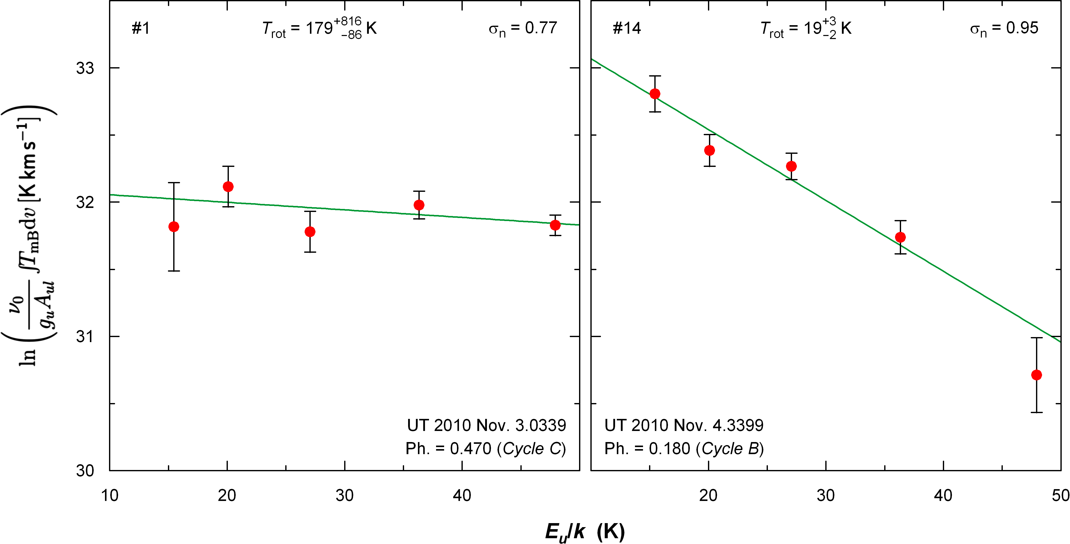
Figure 3: Examples of individual rotational diagrams derived from the time series of CH₃OH. The selected diagrams correspond to the maximum (left panel) and minimum (right panel) temperatures $T_{\mathrm{rot}}$, calculated from the slopes of the weighted linear least-squares fits (solid lines). Note that the error bars associated with the individual data points in both diagrams do not include the uncertainty of the telescope pointing, which affects all five lines almost identically in the framework of the assumed model scenario, and therefore does not affect the slope (although it does affect the zero level). We also show a normalized standard deviation from the fit $\sigma_{\mathrm{n}}$ (for an ideal fit $\sigma_{\mathrm{n}}=0$, for deviations ideally consistent with the errors $\sigma_{\mathrm{n}}=1$, and when the measurements deviate from the model $\sigma_{\mathrm{n}}>1$). The complete set of rotational diagrams is presented in Fig. 12 (Appendix B).

We applied the rotational diagram technique (see Appendix A; also e.g. Bockelée-Morvan et al., 1994) to our time series of CH₃OH to determine the rotational temperature $T_{\mathrm{rot}}$ and its temporal variation. Selected examples of the rotational diagrams are presented in Fig. 3. The errors on $T_{\mathrm{rot}}$ were not derived directly from the temperature variation in the simulated spectra (cf. Section 2), but indirectly, from the variation of the rotational-diagram slopes in these simulations. This change is motivated by the fact that some of the simulations generated for the flattest rotational diagrams (i.e. implying the highest $T_{\mathrm{rot}}$) yield marginally positive slopes (i.e. non-physical temperatures), however, the temperature limits calculated from the slope RMS are physical in all cases. Note that the errors on $T_{\mathrm{rot}}$ do not account for deviations from the model (predicting linear rotational diagrams) but are entirely established by the noise in our data (cf. Section 2).

According to Biver et al. (2002a), the observed group of transitions at $\sim 157$ GHz yields a rotational temperature very close to the kinetic temperature of the inner coma. The two temperatures are strictly equal in Local Thermodynamic Equilibrium (LTE), in which the energy levels are populated according to the Boltzmann distribution, and the resulting rotational diagrams are linear. Indeed, the majority of our rotational diagrams are indistinguishable, within the error bars, from being linear, although in some cases we observe strong nonlinearities or accidental deviations. While we cannot exclude instrumental effects (e.g. such as imperfect removal of the baselines) in the spectra behind these problematic diagrams, the possibility of large deviations from the Boltzmann energy-level distributions at these particular rotation phases cannot be ruled out at this stage.

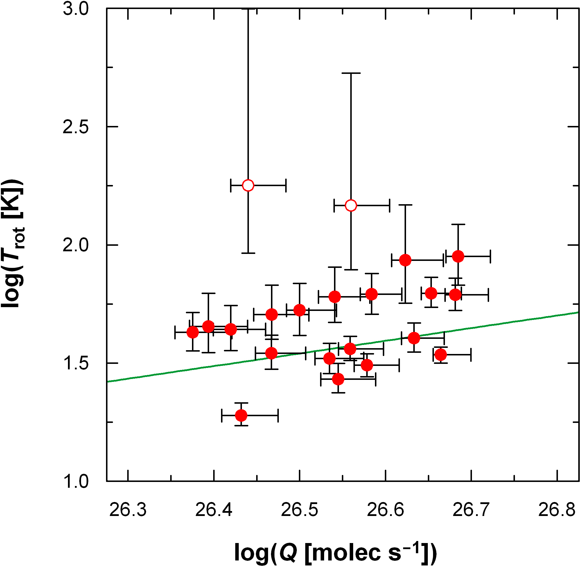
Figure 5: Tentative positive correlation of the rotational temperature $T_{\mathrm{rot}}$ (Fig. 4) and the production rate $Q$ (Fig. 8), derived from the time series of CH₃OH, and presented in log–log scale. The weighted linear least-squares fit (solid line) is added to guide the eye. It was obtained with the weights iteratively calculated from relevant (positive or negative) sides of the vertical and horizontal error bars. The fit has a slope of $0.54_{-0.24}^{+0.19}$, where the errors were estimated from the variation of the slope in the set of simulated spectra (cf. Section 2). The two highest-temperature data points (open symbols) were rejected from the fit because many of the simulations yield non-physical temperatures for these points and for the same reason five simulations (from the set of 500) were omitted from the error estimation, as they yield non-physical temperatures for other data points. We conclude that this positive correlation must be real given that negative slopes appear only in 1.6% of the simulations. We also note that the two rejected data points have a small influence on the slope, which is equal to $0.50$ for the complete dataset.

The temporal behavior of $T_{\mathrm{rot}}$ is presented in Fig. 4. We see large-amplitude variations that seem to generally follow the rotation-modulated production rate (see further Fig. 8 and the discussion in Section 4.1), although the correlation is not strict. While, again, occasional instrumental effects might have affected this trend, it seems extremely unlikely that the entire variability is an artifact. Instead, we believe that the variations are physical and their correlation with the production rate is real (Fig. 5), but additional fluctuations in the rotational temperature are superimposed on the regular trend. It is interesting to note that although a positive correlation of these two quantities has been predicted by theory (e.g. Combi et al., 2004), only the correlations in long-term trends, primarily controlled by changing heliocentric distance, have been reported for individual objects to date (e.g. Biver et al., 2002a). Our result suggests that the rotational temperature can be positively correlated with the production rate in a single object also when the received solar energy flux is constant.

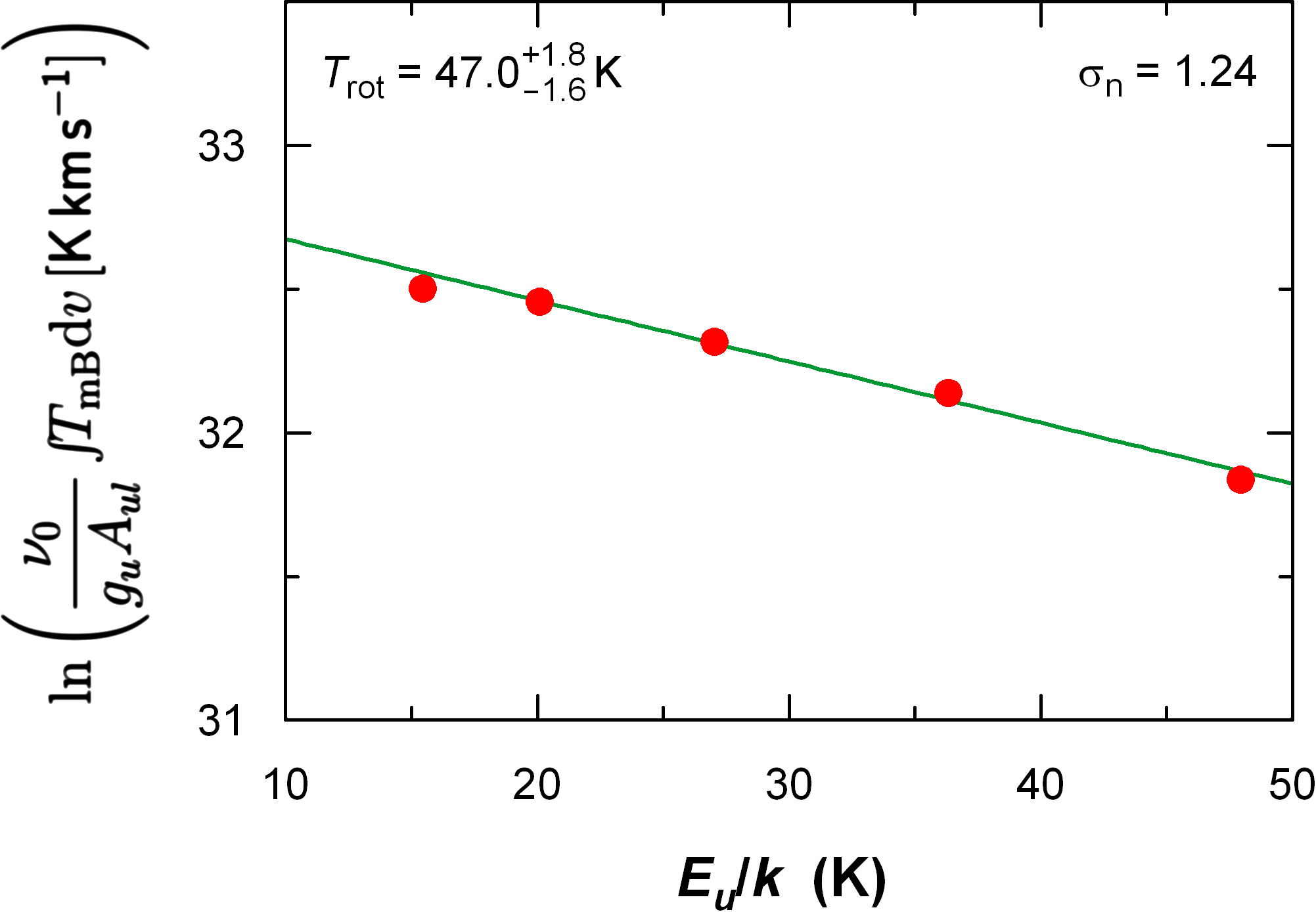
Figure 6: Rotational diagram for the mean spectrum of CH₃OH from Fig. 1. The error bars are smaller than the symbol size. Other details are the same as in Fig. 3.

We also calculated a rotational diagram for the mean spectrum from Fig. 1. The diagram, presented in Fig. 6, is consistent with the temperature of $47.0^{+1.8}_{-1.6}$ K. While this value is some 30 K lower than the rotational temperatures from IR spectroscopy (Mumma et al., 2011; Dello Russo et al., 2011), the latter were derived from a much smaller volume surrounding the nucleus, where the gas has presumably the highest temperature (e.g. Combi et al., 2004), and hence this difference should be expected and in fact was often noticed in the past (e.g. Drahus et al., 2010). It is important to realize that the gas observed by our beam was presumably highly non-isothermal, both in time (see above) and across the coma (e.g. Combi et al., 2004), even if it locally satisfied LTE. Moreover, we cannot exclude that non-thermal processes significantly contributed to the overall excitation scheme, especially in the outer part of the observed coma. Therefore, interpretation of the rotational temperature in such an environment is highly problematic and some of these problems will be discussed by Drahus et al. (in prep.).

4 Sources of HCN and CH₃OH

4.1 Average Production Rates and Temporal Variability

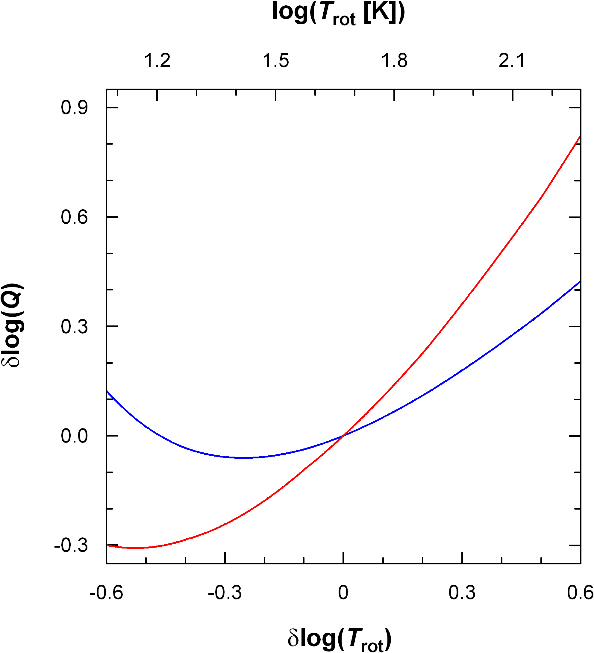
Figure 7: Dependence of the derived production rate $Q$ on the adopted rotational temperature $T_{\mathrm{rot}}$, presented as logarithmic offsets applicable to CH₃OH (red) and HCN (blue). The absolute logarithmic temperature scale is given by the upper horizontal axis.

Both the average and the instantaneous production rates $Q$ were derived from the line areas $\int\!\!T_{\mathrm{mB}}\mathrm{d}v$ assuming a constant gas expansion velocity $v_{\mathrm{gas}}=0.8$ km s^-1 and using the average rotational temperature $T_{\mathrm{rot}}=47$ K (Section 3). At this point we refrain from using the instantaneous $T_{\mathrm{rot}}$ for the calculation of the instantaneous $Q$, because of the relatively large errors on the individual temperatures (especially on the highest ones), the uncertain reason(s) for the occasional nonlinearities of the rotational diagrams, and some uncertainty as to the cause(s) of the observed variability (cf. Section 3). In Fig. 7 we show how the derived production rates depend on the adopted rotational temperature. We also note that in the framework of our simple model the production rate is a linear function of the line area, and that we used constant in time conversion factors for the two molecules (cf. Appendix A).

The derived average absolute production rates are $3.5\times 10^{26}$ molec s^-1 for CH₃OH and $1.25\times 10^{25}$ molec s^-1 for HCN. The production-rate ratio is 28, which is some 50% higher than the most typical values found in comets from millimeter spectroscopy (Biver et al., 2002b). The derived ratio is also noticeably higher than the values of 6–9 resulting from the measurements of 103P by Mumma et al. (2011) and Dello Russo et al. (2011) obtained in the infrared (and updated with the revised IR production rates of CH₃OH by Villanueva et al., 2012), but such an inconsistency should again be no surprise, given all the differences in data acquisition and modeling, and also the natural variability of this comet.

We observe well-defined variation in the instantaneous production rates of both molecules (Fig. 8), which we previously noticed in HCN and connected with the rotation of the nucleus (Paper I). The two time series correlate remarkably well although the amplitudes are different, reaching a factor of 4 for HCN but only a factor of 2 for CH₃OH. However, the measured amplitudes can differ from the real ones if some of our model assumptions (Appendix A) are strongly violated, in particular (i) the negligible optical depth, (ii) the constant rotational temperature, or (iii) the outgassing properties.

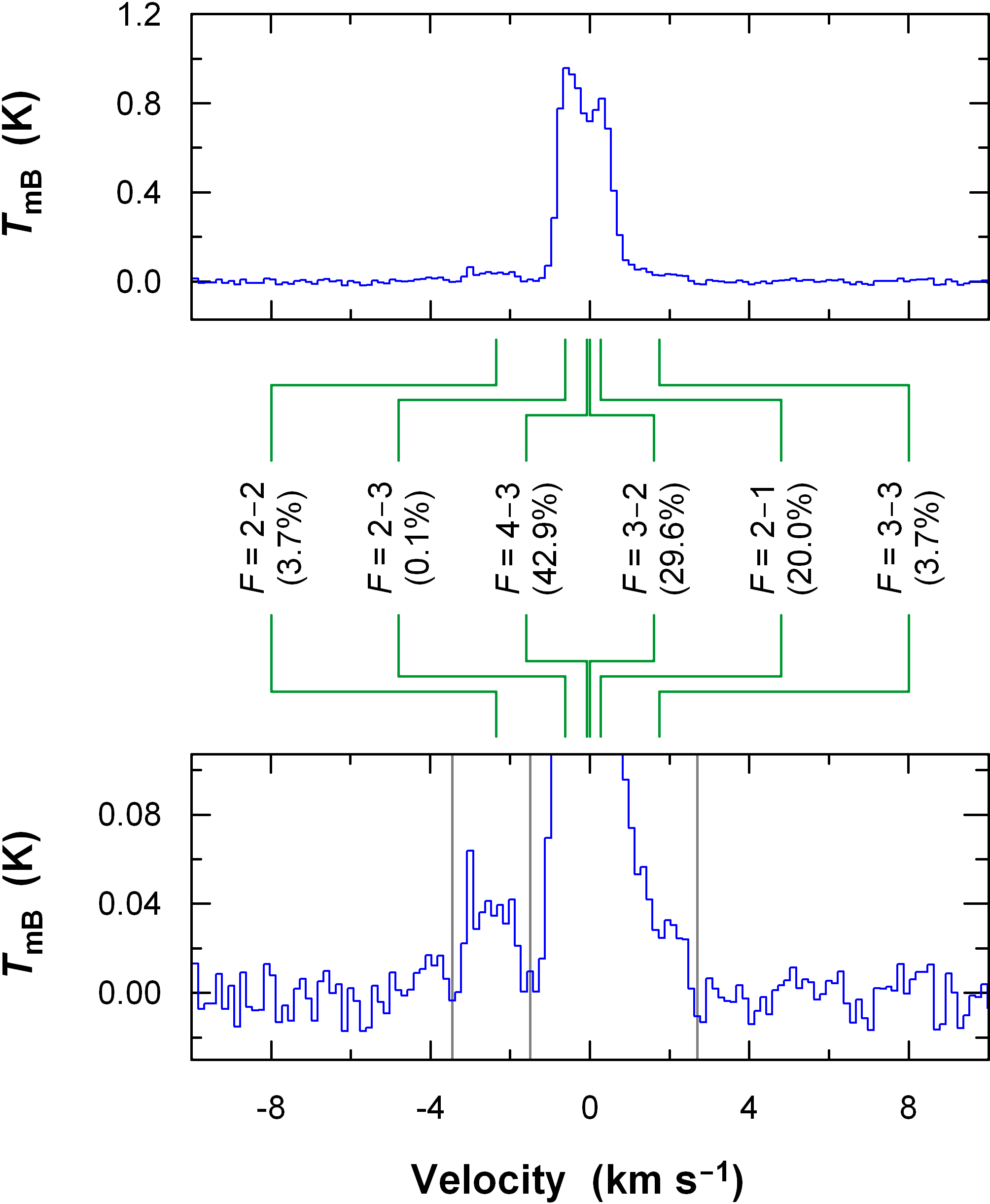
Figure 2: Mean spectrum of HCN J(3–2) resulting from the 21 spectra in our time series. The top panel shows the complete line profile whereas the bottom panel shows a close-up view of the baseline. The solid lines between the panels indicate the velocities of the hyperfine components taken from the Cologne Database for Molecular Spectroscopy (Müller et al., 2005); they are labeled and their theoretical branching ratios are given in the brackets. It is evident that, in addition to the three strongest hyperfine components which build up the line, two faint components are also visible: one fully resolved at $-2.3545$ km s^-1 ($F=2-2$) and the other one in the red wing of the line at $+1.7394$ km s^-1 ($F=3-3$). The vertical lines in the bottom panel indicate the velocity ranges in which we measured the component ratio (Section 4.1).

A non-negligible optical depth would lead to an underestimation of the production rates, most significant for the brightest lines. Consequently, the amplitude of the brighter HCN would be reduced compared to the fainter CH₃OH, and since we observe otherwise, the real amplitude difference would have to be higher than measured. Nevertheless, the optical depth is completely negligible in our data, which is best evidenced by the hyperfine splitting of the HCN J(3–2) line (Fig. 2). We make use of the fact that the relative intensities of the hyperfine line components in a single molecule are established by fundamental physics and do not depend on the excitation conditions or mechanisms (e.g. Bockelée-Morvan et al., 1984). Consequently, if a component ratio measured in a molecular environment is equal to the theoretical value for a single molecule and different from unity, it implies that these components are optically thin. Taking advantage of the exceptionally high signal-to-noise ratio in the average spectrum of HCN, we can easily distinguish the $F=2-2$ hyperfine component and measure its area (from $-3.45$ to $-1.5$ km s^-1) separately from the blend of the remaining components (from $-1.5$ to $+2.7$ km s^-1). We find the component ratio to be equal to $24.1^{+1.5}_{-1.3}$ which is consistent with the theoretical ratio of 26.0 (cf. Cologne Database for Molecular Spectroscopy; Müller et al., 2005). This means that even the brightest region of the line, which is always first to saturate, is practically free of self-absorption, and that the fainter lines of CH₃OH must be optically thin as well.

Since the production rates were derived using the constant rotational temperature, they can be naturally affected by the measured temperature variations (Section 3). From the theoretical relation between these two quantities in Fig. 7 we see that the derived production rate depends on the temperature more strongly for CH₃OH than for HCN. This implies that the variations of the line area could not have been produced primarily by the varying temperature instead of the production rate because the amplitude would be higher in CH₃OH than in HCN. Consequently, it must be a real variability of the production rate generating physical changes in the rotational temperature rather than the temperature variations modulating our derived production rates. However, the latter effect must also be present to some extent. Bearing in mind the suspected positive correlation of these two quantities in our data (Fig. 5), we expect that the derived production-rate maxima are somewhat underestimated and the minima overestimated, although this reasoning is limited to $T_{\mathrm{rot}}>26$ K for which both functions in Fig. 7 monotonically increase (a lower $T_{\mathrm{rot}}$ was measured in only one data point, spectrum #14, and is equal to 19 K). Consequently, the observed amplitudes can be lower compared to the real ones, and since the effect is stronger for CH₃OH than for HCN, it can explain, at least to some degree, the different amplitudes measured in our data.

In the above discussion we assumed that the temperature variation is the same in HCN and CH₃OH. If, instead, the (unmeasured) characteristic temperature applicable to our HCN data varied more strongly, e.g. due to the smaller beam size (Table 1), the range of the production-rate offsets from Fig. 7 could even exceed the range for CH₃OH. This would imply that the real production-rate amplitudes differed more than inferred from our data because HCN would be attenuated more strongly than CH₃OH. On the other hand, this scenario still cannot explain the derived production-rate variations as artifacts caused by the varying temperature (even though correctly implying the measured amplitude relation) because in such a case the two quantities would be inversely correlated while the determined correlation is straight. Whereas the situation can be, in principle, even more complex if e.g. the two variability profiles of $T_{\mathrm{rot}}$ were totally different, we believe, rather, that the beam-size effect is of secondary importance in this respect – and hence the temperature in the data of both molecules is comparable, as we cannot identify other effects that could differentiate it significantly.

However, the different beam sizes can also affect the derived production rates in other ways, especially when the outgassing properties assumed in the model (Appendix A) are strongly violated. In fact, the outgassing of 103P is by no means in steady state and isotropic, but rather dominated by rotating jets and icy grains periodically injected into the coma (see the next sections and references therein). In such a case, the observed amplitude can be smaller than the real one, by a factor which depends on the sublimation-time dispersion of the molecules contributing to a single spectrum (see e.g. Biver et al., 2007; Drahus et al., 2010). In this way, the lower amplitude of CH₃OH seems to be naturally explained, given the larger beam size that effectively “sees” the molecules from a broader range of nucleus rotation phases compared to the smaller beam of HCN (Table 1). But this simple reasoning fails to explain the remarkable temporal correlation of both variability profiles, and also the fact that the maxima and minima look relatively flat. Consequently, the timescale of variations appears sufficiently long compared to the integration time and escape time from the beam (both $\sim 1$ hr) to ensure that the outgassing properties are rather “frozen” on the spatial and temporal scales characteristic of the individual CH₃OH and HCN data points (Table 1). This may indicate that the two diurnal amplitudes were indeed different. However, even if they were the same, the different beam sizes would still differentiate them in the same sense as observed if, for example, the minimum level was produced by a constant background with uniform brightness distribution, i.e. if the model assumption of a central source of outgassing is not well satisfied. (Note that the production-rate profiles of CH₃OH and HCN are still deformed by the outgassing anisotropy, but both in a similar way.)

Last but not least, we note that the errors of telescope pointing can also affect the derived production-rate profiles. Since the effect is inversely correlated with the beam size, it affects HCN more strongly than CH₃OH, but in the same sense, and therefore it is consistent with their seeming temporal correlation and the relation of their amplitudes. However, given that the pointing corrections were always determined between the consecutive points in the time series, this effect is practically incapable of generating entire trends, introducing only small random deviations, and also its expected magnitude is rather small which is reflected by the derived error bars.

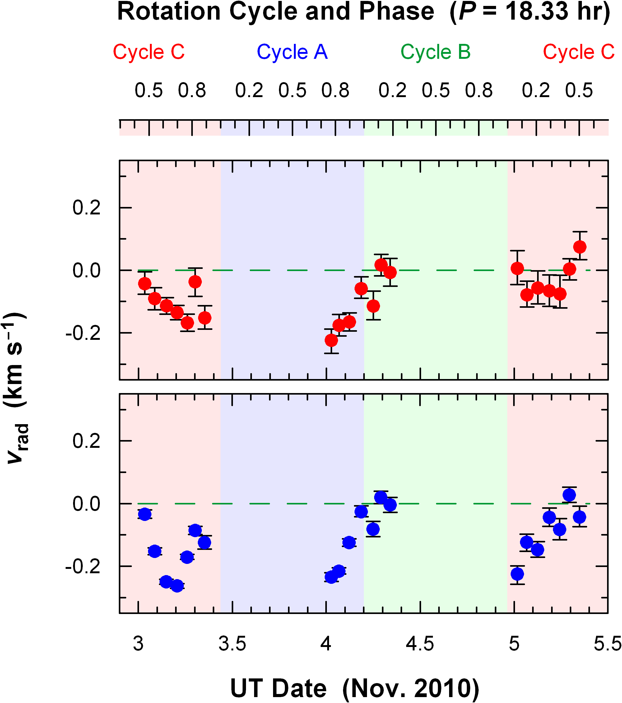
Figure 9: Variability of the median radial velocity $v_{\mathrm{rad}}$ in CH₃OH (top panel) and HCN (bottom panel) about the rest velocity (dashed lines). The uncertainty of the telescope pointing is assumed to have a negligible influence on this parameter and hence the errors result entirely from noise (Paper I). The additional top axis shows the nucleus rotation phase and three-cycle component (cf. Paper I), and the latter is also coded by the background color. The EPOXI flyby occurred on UT 2010 Nov. 4.5832, corresponding to phase 0.5 of Cycle B.

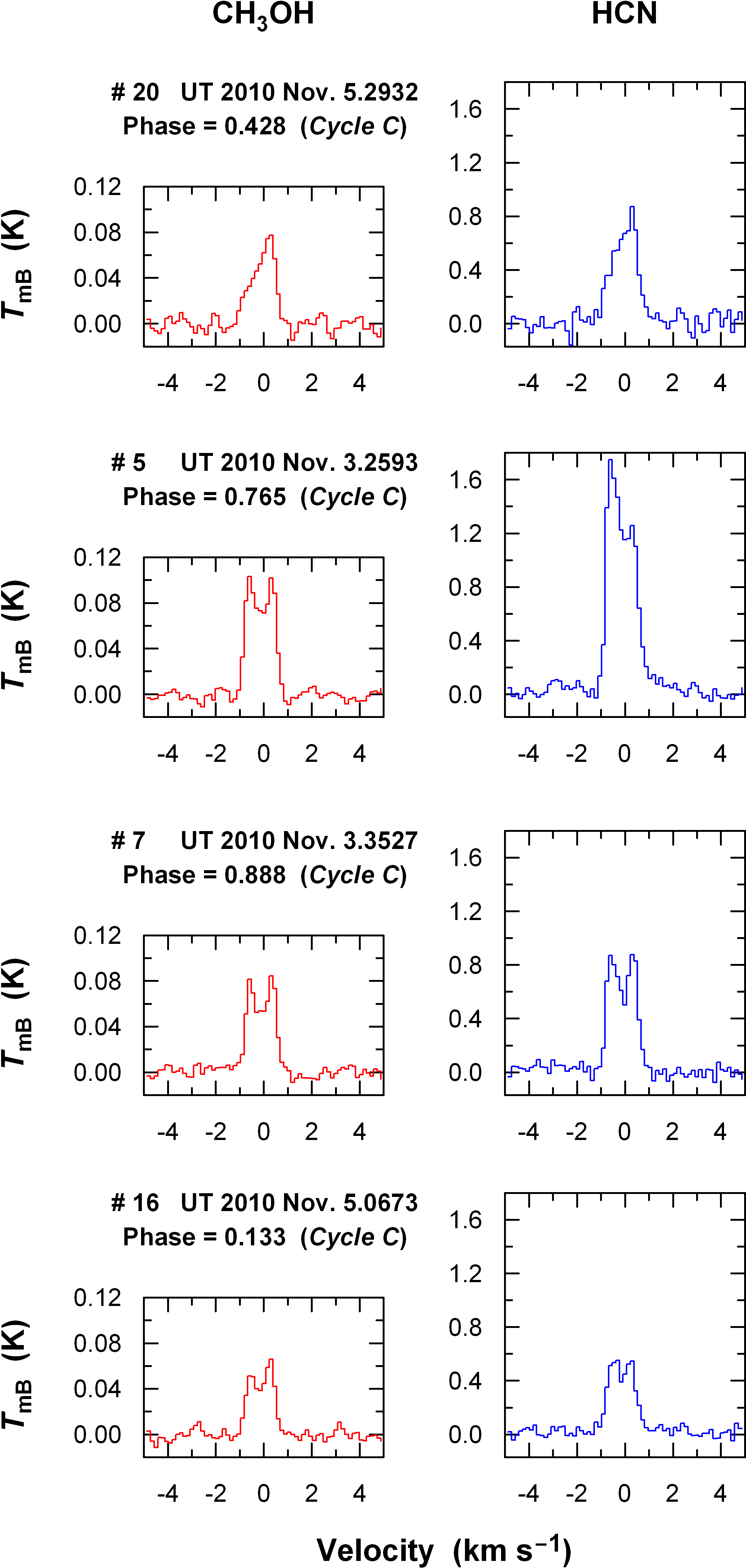
Figure 10: Examples of the line profiles of CH₃OH (left panels) and HCN (right panels) illustrating the temporal variations as the nucleus rotates (from top to bottom). The former are the mean profiles from the observed five lines whereas the latter are the profiles of the J(3–2) transition (Section 2 and Table 1). We selected four representative rotation phases from two consecutive Cycles C (cf. Paper I) observed on UT 2010 Nov. 3 (middle panels) and Nov. 5 (top and bottom panels). The complete dataset is presented in Fig. 13 (Appendix B).

In order to fully understand the characteristics of the two production-rate profiles, we need to take into account the velocity information naturally contained in the lineshapes. Figure 9 shows the variability of the median radial gas-flow velocity $v_{\mathrm{rad}}$, which has been assumed equal to the median line velocity $v_{0}$ (Appendix A). The behavior is also well defined and consistent with the rotational periodicity of the nucleus. We see that the line-of-sight kinematics were noticeably different for the two molecules, in particular, HCN drifts towards deeply blueshifted velocities around the phases of maximum activity, while the velocities of CH₃OH change less. In Fig. 10 we show examples of the individual lineshapes. A close-up look reveals that HCN has a strong blueshifted component at the active phases, while CH₃OH looks symmetric with two distinct peaks. The difference vanishes at the interim and quiescent phases, at which the lineshapes look remarkably similar to each other – featuring two symmetric peaks which resemble the lineshape of CH₃OH at the active phases (although the redshifted peak occasionally dominates the spectra of both molecules). The implication of these differences is that the sources of the two molecules must have differed in some way. We further explore this inference in the next section.

4.2 Interpretation of the Lineshapes

4.2.1 Basics of Lineshape Interpretation

Since the characteristic gas-flow velocity in comets 1 AU from the Sun is $\sim 1$ km s^-1 (e.g. Combi et al., 2004), our spectra are fully “velocity resolved” given that the spectral resolution is 0.15 km s^-1 (Section 2). The lineshapes in such spectra are primarily controlled by the Doppler effect. Other effects, including optical depth and hyperfine structure, can also theoretically influence the lineshapes but are negligible in our data. The velocity-calibrated spectra can be hence identified as histograms, showing how the molecules observed within the beam are distributed in radial velocity, weighted by the emission coefficient (which is a function of the excitation conditions in different regions of the coma).

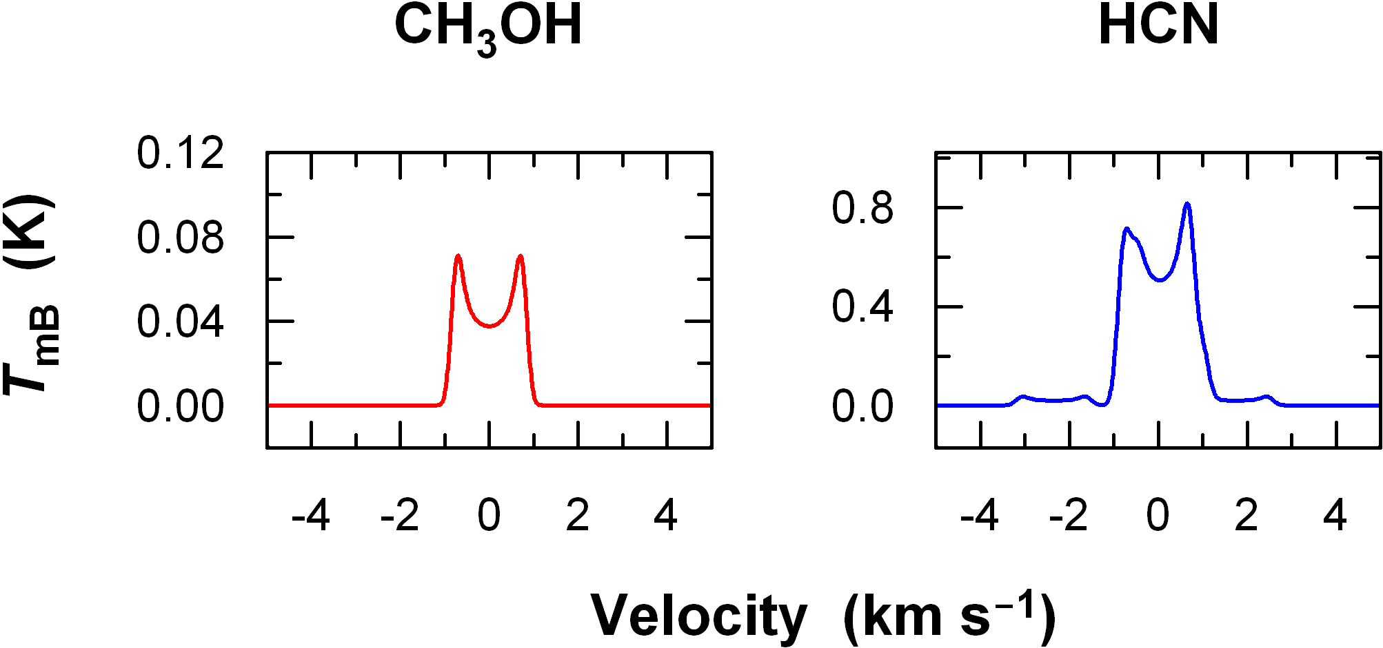
Figure 11: Simulated spectra of CH₃OH (left panel) and HCN (right panel) for steady-state isotropic outgassing from a central source with the physical and geometric conditions compatible with our data. We used the production rates of $3.5\times 10^{26}$ and $1.25\times 10^{25}$ molec s^-1, respectively (Section 4.1), a constant gas-flow velocity of 0.8 km s^-1 (Appendix A), and LTE at 47 K (Section 3). The beam sizes and the molecular constants were used the same as given in Table 1 (Section 2). The HCN profile additionally accounts for the hyperfine structure taken from the Cologne Database for Molecular Spectroscopy (Müller et al., 2005), which introduces the asymmetry. This information is currently unavailable for the observed lines of CH₃OH, and hence the mean model profile is symmetric.

This distribution depends on the directions in which the molecules travel. In particular, molecules traveling along the line of sight are either maximally redshifted or blueshifted, while molecules traveling normal to the line of sight are observed at zero velocity (corresponding to their rest frequencies). If the molecules are ejected isotropically at a constant speed, then the emission line should feature two peaks symmetrically located about 0 km s^-1, with radial velocities equal to the positive and negative values of the gas-flow velocity (see model examples in Fig. 11). This is because most molecules in the beam travel either towards or away from the observer along the line of sight. Molecules traveling perpendicular to the line of sight leave the beam fastest producing a central minimum in the line profile. Moreover, real gas always has a “thermal” velocity component that blurs the lineshape. This effect is of secondary importance, however. For example, the thermal speed of CH₃OH at 47 K (Section 3) is only 0.2 km s^-1, small compared to the bulk gas-flow velocity of $\sim 1$ km s^-1.

The travel directions of the molecules, at least in the inner coma, can be identified with the directions in which they were ejected, and therefore, in the discussion below, we directly link the observed spectral features with the characteristics of 103P’s outgassing. At this stage we only aim at interpreting the most obvious spectral features and only in a qualitative manner. A more in-depth analysis requires a detailed lineshape modeling (cf. Drahus, 2009), which is presently in preparation.

4.2.2 Evolution of the Lineshapes

The evolution of the lineshapes (see Fig. 10) can be grouped in three distinct ranges of the nucleus rotation phase:

• Phases 0.4–0.5 (spectra #1 and #20–21): the redshifted jet.

  The line profiles of CH₃OH and HCN look very similar. They feature a well-defined redshifted peak at about $+0.3$ km s^-1, which we identify with a jet directed away from the Earth (as projected onto the line of sight). The gas in the jet was abundant in both CH₃OH and HCN, and must originate from a vent (or a group of vents) on the nucleus, which was active only at these particular rotation phases. We refer to this feature as to the redshifted jet.

• Phases 0.5–1.0 (spectra #2–7, #8–11, and #21): the blueshifted jet.

  Essentially half of the rotation cycle, between phases 0.5 and 1.0, is dominated by the appearance of a second jet (this time blueshifted) and associated phenomena:

  • The first signatures are visible in HCN around phase 0.5. The HCN lineshape starts showing a blueshifted peak, which is visible simultaneously with the redshifted peak from the earlier jet (spectrum #21, and between #1 and #2). At the same time, CH₃OH still shows only the redshifted peak.

  • Around phase 0.55 (spectrum #2) the blueshifted peak starts dominating the HCN spectrum, while CH₃OH becomes symmetric with two distinct peaks.

  • Between phases 0.6 and 0.8 (spectra #3–5 and #8–9) both molecules rapidly brighten while their lineshapes continue to starkly differ from each other: HCN is totally dominated by a blueshifted peak near $-0.6$ km s^-1 and CH₃OH shows two rather equal peaks located symmetrically about $-0.15$ km s^-1 (one close to $-0.6$ km s^-1 and the other one near $+0.3$ km s^-1).

  • After reaching the maximum brightness around phase 0.8, both molecules start fading until about phase 1.0 (spectra #6–7 and #10–11). This changeover is associated with a dramatic transformation of the HCN lineshape. It starts showing two symmetric peaks, just like CH₃OH that remains unchanged, and so the lineshapes of the two molecules look very similar while the brightness decreases.

  The lineshapes dominated by the blueshifted peak at about $-0.6$ km s^-1 can be identified with a jet originating from a vent (or a group of vents) on the nucleus, which was active only at these particular rotation phases. The gas was produced Earthward as projected onto the line of sight, and hence we refer to this feature as to the blueshifted jet. On the other hand, the symmetric double-peak lineshapes, blueshifted by $\sim 0.15$ km s^-1, can be most easily interpreted as created by an isotropic source, also moving Earthward (in the same sense as above) but about four times slower than the gas in the jet.

  We associate the isotropic source with ice particles in the coma of 103P. The EPOXI flyby revealed large icy grains close to the nucleus, up to 10–20 cm in radius (A’Hearn et al., 2011), and also the Arecibo radar detected centimeter to decimeter grains (Harmon et al., 2011). However, the velocities of these chunks, mostly below $0.5$ m s^-1 in the EPOXI data and of the order of few to tens of meters per second as measured at Arecibo, are too low to cause a measurable line shift in our spectra. Instead, we believe that the total sublimation area of the grains was controlled by the finest particles (cf. A’Hearn et al., 2011), which were ejected at higher speeds and further accelerated by the gas in the coma. For example, taking the grain velocity as a function of size as derived for this comet from the radar data (Harmon et al., 2011), we obtain $0.2$ km s^-1 for particles $\sim 0.5$ mm in diameter. Such grains would be isothermal and could survive for perhaps an hour at this heliocentric distance, which altogether makes them excellent candidates to explain the symmetric double-peak line profiles and their rapid temporal evolution.

  The grains appear to be injected into the coma and further accelerated by the gas in the blueshifted jet. Consequently, the velocity projection onto the line of sight was basically the same for the gas and ice in the jet, and hence we identify their Doppler-shift ratio of $\sim 4$ with the actual gas-to-grains speed ratio. We also suppose that the projection effect was not very strong for this jet (see further in Section 5), implying that the submm grains traveling at $\sim 0.2$ km s^-1 could also plausibly explain the amount of the systematic blueshift in the double-peak line profiles.

  The spectra show that the gas originating directly at the vent was rich in HCN but not in CH₃OH. In contrast, the excavated ice particles sublimated isotropically and carried abundant HCN and CH₃OH in proportions comparable to the gas in the redshifted jet observed earlier. Consequently, at these rotation phases, the observed HCN sublimated both from the icy grains and from the active vent, while the observed CH₃OH sublimated only from the ice particles. The composition of the grains appears then dramatically different from the composition of the gas in the blueshifted jet which carried them away from the nucleus.

  The above conclusions are consistent with the temporal evolution of both line profiles. At the onset of the blueshifted jet, the observed HCN coma was dominated by the gas in this jet, and therefore the HCN line displays the strongly blueshifted peak. However, at the same time, the observed coma of CH₃OH was dominated by the gas sublimating from the first grains in the jet, and therefore CH₃OH started brightening with some delay, presenting the subtly blueshifted symmetric double-peak lineshape. With time, the grains became more abundant in the coma, and also the outgassing rate from the vent increased, injecting more gas and ice. This corresponds to the rapid brightening visible for both molecules and explains why their profiles continued to differ so much: CH₃OH, sublimating only from the grains (isotropically), preserved the two rather equal peaks, while HCN, produced additionally in the active vent (anisotropically), continued to be dominated by the single peak. At some point, the sublimation from the vent declined, but the ice particles emitted earlier persisted, and that is when the lineshapes of CH₃OH and HCN became strikingly similar to each other, showing two symmetric peaks. While the grains continued to lose their total cross-section and move away from the beam center, the lines kept fading although their shapes remained unchanged.

• Phases 0.0–0.4 (spectra #12–19): the quiescent rotation phases.

  The CH₃OH and HCN lineshapes look rather similar. In most of the spectra, they show the subtly blueshifted symmetric profiles, which we have earlier identified with the isothermal icy grains. The brightness of the lines stabilized at some minimum level, i.e. neither strongly declined with the increasing rotation phase nor rose up with the increasing count of the rotation cycles. This leads us to the conclusion, that the total sublimation area of these particles was fairly constant on a rotation-cycle timescale. Some of the grains perhaps originated from the earlier rotation phases, but this source must have been quickly decaying after deactivation of the blueshifted jet, because of the mass loss from sublimation and decreasing telescope sensitivity as the particles moved away from the beam center. The grains must have been replenished by other sources, perhaps including weaker vents (apparently incapable of generating strong jet signatures in our spectra) or fragmentation of larger chunks with subsequent acceleration of the created particles by the gas in the inner coma.

4.2.3 Additional Remarks

The proposed scenario naturally explains the observed characteristics of the HCN and CH₃OH production-rate profiles (Section 4.1). Bearing in mind that the observed lines reacted almost instantly to the changes in comet’s activity (cf. Section 4.1), the remarkable correlation between the two molecules is understandable given that their maxima are controlled by the same source of activity (the blueshifted jet containing gas and ice) and likewise for the minima (controlled by the background of icy grains). Simultaneously, the difference between the production-rate amplitudes is explained by the HCN excess at the phases of maximum activity, causing a larger range of variation compared to CH₃OH. Other scenarios, which are discussed in Section 4.1, cannot be accepted because they fail to explain the observed differences in the lineshapes. Specifically:

• The varying optical depth can, in principle, produce temporal changes in the line profiles, but we concluded that both molecules were optically thin in our data.

• The variations in the rotational temperature are rather difficult to connect with the lineshapes.

• Potential problems with pointing are unlikely to generate systematic trends or, for the still stronger reason, periodic trends.

• In the suspected situation in which the production-rate amplitudes are differentiated by the different beam sizes (due to background) but the sources of CH₃OH and HCN in the comet are the same, CH₃OH would also display a blueshifted component at the phases dominated by the blueshifted jet (albeit somewhat fainter than in HCN) but we do not see it in our data.

• We also note that the line profiles of CH₃OH and HCN naturally differ due to the presence of hyperfine splitting, but this difference is “static” for optically-thin lines and rather small (Fig. 11).

While none of the above mechanisms can be a plausible alternative to the postulated difference in the sources of CH₃OH and HCN, some of them could possibly be held responsible for small deviations from our preferred scenario, which naturally exist in our data. Small inconsistencies could also be attributed to the weaker outgassing sources observed by EPOXI (A’Hearn et al., 2011), to the non-trivial dynamics of the comet’s coma, and also to the reported excitation of the nucleus rotation state (cf. Paper I; also A’Hearn et al., 2011; Knight & Schleicher, 2011; Samarasinha et al., 2011; Waniak et al., 2012) which we explore in the next section. When attempting to identify the smallest inconsistencies, one should also keep in mind some unavoidable limitations of our dataset, such as the finite signal-to-noise ratio and baseline reliability, and the limited pointing accuracy of the telescope, as well as the rotation-phase errors possibly caused by the limited knowledge of the rotational dynamics of the nucleus.

4.2.4 Differences between Rotation Cycles

It is interesting to note that some well-defined deviations from the picture presented in Section 4.2.2 can be plausibly associated with the excitation of 103P’s rotation state. They also agree remarkably well with the three-cycle scenario that we introduced in Paper I to approximate repeatability in rotation-modulated data of this comet. Specifically:

• Phases 0.1–0.2 (spectra #13–14) on UT Nov. 4 (Cycle B) show that the lines of CH₃OH and HCN are consistently dominated by the redshifted peak, resembling the lineshapes previously identified with the redshifted jet at phases 0.4–0.5 (Section 4.2.2). However, on UT Nov. 5 (Cycle C) the lines at phases 0.1–0.2 (spectra #16–17) are symmetric and fainter than on UT Nov. 4 (Cycle B).

  We suppose that the redshifted lineshapes, appearing at the two separate phase ranges, might have been produced by the same redshifted jet identified earlier. Because of the excitation of 103P’s rotation and the likely circumpolar origin of the redshifted jet (see further in Section 5), the parent vent might have been activated by sunlight at phases 0.4–0.5 during Cycle C, but earlier – at phases 0.1–0.2 – during Cycle B. This interpretation is consistent with the fact that in both cases the lineshapes of CH₃OH and HCN look very similar (unlike at the phases dominated by the blueshifted jet) and is additionally confirmed by the HCN data from UT Nov. 2 (see further in this paragraph).

• The excitation of the rotation state is also likely responsible for the fact that at the rotation phase 0.82 of Cycle C (spectrum #6 obtained on UT Nov. 3) the lineshapes are evidently more evolved than at the same phase of Cycle A (spectrum #9 obtained on UT Nov. 4). Given the remarkable coincidence in phase of the redshifted jet observed during two consecutive Cycles C (Section 4.2.2), the above inconsistency cannot be removed by simply adjusting the 18.33-hr rotation period.

• The spectra of HCN from UT Nov. 2 (formally excluded from the analysis because no counterpart spectra of CH₃OH were taken), covering phases 0.2–0.6 of Cycle B, show that the redshifted and blueshifted jets appeared at relatively earlier rotation phases than in Cycle C observed on UT Nov. 3 and 5. This behavior is consistent with the rotational production-rate profiles of HCN from a much bigger dataset presented in Paper I.

  On UT Nov. 2 the redshifted jet is visible at phases 0.2–0.25, which agrees with the short Cycle B data from UT Nov. 4 (covering phases 0.05–0.2) in which we have identified this jet at phases 0.1–0.2 (see earlier in this paragraph). Combining these two pieces of Cycle B data we conclude that the redshifted jet was present at phases 0.1–0.25, with a subtle local minimum at phase 0.2.

  Moreover, in Cycle B the blueshifted peak looks fainter than in Cycles C and A, which may indicate that the blueshifted jet was physically weaker (e.g. due to different insolation), although other explanations may be possible as well (e.g. a different projection effect). Whatever the cause, in Cycle B the blueshifted jet triggers a comparable quantity of icy grains as in Cycles C and A and, consequently, at the phases of maximum brightness the HCN line features a symmetric double-peak profile.

5 Discussion

The velocity-resolved spectral time series of CH₃OH and HCN reveal a complex outgassing portrait of 103P. We identify outgassing in the form of at least two jets – the redshifted jet and the blueshifted jet – expanding in the opposite directions as projected onto the line of sight and having seemingly different compositions. The blueshifted jet appears as a strong source of HCN gas and of icy grains, but not of CH₃OH gas. The composition of the grains is, however, dramatically different from the composition of the gas in this jet because, in addition to HCN, they also contain large amounts of CH₃OH. Surprisingly, in terms of composition the grains are very similar to the gas in the redshifted jet, which is also rich in HCN and CH₃OH although it does not carry much ice. Consequently, the origin of the observed CH₃OH and HCN can be summarized as follows:

• CH₃OH:

  • anisotropic sublimation from the active vent that produced the redshifted jet,

  • isotropic sublimation from the icy grains carried away primarily in the blueshifted jet, but not from the vent itself (at least not at any measurable level).

• HCN:

  • anisotropic sublimation from the active vent that produced the redshifted jet,

  • anisotropic sublimation from the active vent that produced the blueshifted jet,

  • isotropic sublimation from the icy grains carried away primarily in the blueshifted jet.

It is interesting to note that, at the comet’s phase angle $\sim 60\arcdeg$ (Section 2), the Sunward direction projects as blueshifted and most of the illuminated part of the nucleus would emit material in the blueshifted directions. However, a smaller but still substantial fraction of the illuminated part would emit material in the redshifted directions. For this reason, it is entirely possible that both the vent producing the blueshifted jet and the vent producing the redshifted jet were illuminated while being active. However, we suppose that the redshifted jet originate from a vent close to the region of the polar night, which was illuminated only during a short fraction of the rotation cycle. This would naturally explain its short duration and opposite radial-velocity component compared to the blueshifted jet. Supposing that the gas-flow velocity was comparable in the two jets, perhaps close to 0.8 km s^-1 (Appendix A), we take into account the difference in velocity offsets of the line peaks ($+0.3$ km s^-1 for the redshifted jet vs. $-0.6$ km s^-1 for the blueshifted jet) and conclude different significance of the projection effect – implying that the blueshifted jet was emitted in a direction close to the line of sight, while the redshifted jet was relatively closer to the sky plane. We note that the fact that the two seemingly different jets appeared at consecutive rotation phases makes them hard to distinguish in the time series of the total production rate (Fig. 8). However, expanding in the opposite directions (as projected onto the line of sight), they clearly manifest themselves as separate features in the velocity-resolved line profiles.

The properties of these two jets resemble very much the CN features observed around the same time in narrowband optical images (Knight & Schleicher, 2011; Samarasinha et al., 2011; Waniak et al., 2012). In particular, the images of Waniak et al. (2012) – obtained nearly simultaneously with our IRAM 30 m data – are dominated by structures with low projected sky-plane velocities, hence expanding close to the line-of-sight direction (the slow CN feature). We tentatively associate these features with our blueshifted jet, given the dominating role of the blueshifted jet in our data and also its strong Doppler shift. However, a small part of the dataset of Waniak et al. (2012) shows a much faster feature, expanding in the S–SW direction (the fast CN feature) probably not far from the sky plane. Interestingly, Knight & Schleicher (2011) and Samarasinha et al. (2011) report that the S–SW feature became first visible only in October. Therefore, we suppose that it is the same structure as our redshifted jet, having a relatively weak Doppler shift, and probably just emerging from the polar night.

We have earlier established (Paper I) that the variability of the HCN production rate was in phase with the brightness variation in CO₂ and H₂O observed by EPOXI (A’Hearn et al., 2011). Therefore, CH₃OH also correlates with all these molecules. But even though the variations of the four molecules were in phase, the spatially resolved molecular observations from EPOXI revealed different reservoirs of CO₂ and H₂O, and our own observations show differences between HCN and CH₃OH. Interestingly, however, the variability amplitudes of HCN and CH₃OH, reaching a factor of 4 and a factor of 2, respectively, are the same as measured for CO₂ and H₂O. An intriguing hypothesis arises then, that perhaps HCN is spatially correlated in the nucleus with CO₂ and CH₃OH with H₂O. Consequently, we suppose that the redshifted jet (tentatively associated with the fast CN feature) was observed by EPOXI as the water jet, while the blueshifted jet (tentatively associated with the slow CN feature) was observed by the spacecraft as the carbon dioxide jet. Moreover, the carbon dioxide jet is the main supplier of icy grains in the EPOXI data (A’Hearn et al., 2011) and the same is true for the blueshifted jet in our data.

At this stage it is difficult to accurately quantify how much gas originated directly at the nucleus and how much was produced from the grains in the coma. Nevertheless, taking into account that in about half of the HCN spectra, and in most of the CH₃OH ones, the lines have two symmetric peaks (which we associate with the grains), we can very crudely estimate that probably about half of the HCN molecules, and most of the CH₃OH ones, sublimated from the grains. This conclusion is in agreement with the statement of A’Hearn (2011) based on the EPOXI data. However, we also note that in Cycle B covered on UT Nov. 2 (just one three-cycle before the EPOXI flyby, which occurred at the middle of the next Cycle B), the blueshifted jet appeared weaker than in Cycles A and C, but excavated a comparable amount of ice. Consequently, at phase 0.5 of this cycle, corresponding to the situation at the encounter, the HCN spectra are totally dominated by the icy grains. This may indicate that EPOXI visited 103P when the abundance of ice in the coma was exceptionally high compared to the gas directly sublimating from the nucleus and hence the information inferred from the flyby may not represent the typical behavior of this comet.

It is now our ongoing effort to model the entire set of line profiles in a non-steady-state anisotropic fashion (cf. Drahus, 2009), simultaneously with the image time series of CN (Waniak et al., 2012). We wish to take advantage of the fact that both types of data contain the velocity information in orthogonal dimensions and hence are fully complementary. The result will be used to constrain a 3D outgassing portrait and retrieve the source locations of CH₃OH and HCN, which will be readily comparable with the spatially resolved observations of CO₂ and H₂O from EPOXI. This will enable us to verify the suspected identities of the various features emerging from the different datasets, which are only hypothetical at this stage. We will also better understand the sublimation dependence on insolation, quantify the gas contribution from the icy grains, and obtain realistic, time-dependent absolute production rates and gas-flow velocities.

The compositional heterogeneity with respect to CO₂ and H₂O can be possibly explained by the different characteristic sublimation temperatures: 72 K and 152 K, respectively (Yamamoto, 1985). This should compositionally decouple these two molecules both in the protosolar environment (different locations of the snowlines) and also later, in the thermally processed ices of Jupiter-family comets (Guilbert-Lepoutre & Jewitt, 2011). In contrast, HCN and CH₃OH have practically the same sublimation temperatures, 95 K and 99 K, respectively (Yamamoto, 1985), and therefore the observed heterogeneity may suggest that they underwent different condensation processes. Perhaps HCN can at least partly escape from water ice, while CH₃OH is fully incorporated in it – either in the form of clathrate-hydrates or as trapped gas within the (amorphous) ice matrix (e.g. Prialnik et al., 2004). If true, it seems entirely possible that a part of 103P’s nucleus has been more heated in the past and therefore lost its volatiles except for water and the molecules incorporated in water ice (CH₃OH, HCN, …), and that is where the redshifted jet originates from. At the same time, another part can be more primordial and dominated by free volatiles (CO₂, HCN, …) rather than H₂O and the water-bonded elements, and that is where the blueshifted jet is formed. However, water and the molecules incorporated in water ice are emitted from this part in the form of solid icy grains, and therefore we suppose that they also directly sublimate from this area, but at rates so much lower compared to the free volatiles that they remain undetected.

If this scenario is true, the nucleus of 103P might have been born as a body in which the molecules were uniformly mixed in a bulk sense. In that case we would expect that the redshifted jet was much stronger in the past, when powered by the free volatiles as currently observed in the blueshifted jet. However, in the course of time the thermal evolution of the body reversed the jet strengths. It is suggestive that we currently observe the blueshifted jet on its way to completely lose the free volatiles and become compositionally similar to the evolved redshifted jet but much weaker. This process, if sufficiently fast, may be responsible for the significant decline in activity of 103P compared to the previous return (cf. Combi et al., 2011, albeit measured through a proxy for water). Last but not least, given the above evolutionary constraints, it is more appropriate to characterize the redshifted jet as “HCN-depleted” rather than the blueshifted jet as “CH₃OH-depleted”, although from the observational point of view it seems counterintuitive at first glance.

Our results demonstrate the scientific potential of dense time series of velocity-resolved spectra taken at millimeter wavelengths. We found large-scale heterogeneity of 103P’s nucleus with respect to HCN and CH₃OH, which was not reported by two groups observing independently in the infrared. We suspect that the dense time series of Dello Russo et al. (2011) is too incomplete to show the compositional differences between different parts of the nucleus, as it covers only 17% of the rotation cycle in HCN (two exposures) overlapping with 28% coverage in CH₃OH (five exposures). The sparsely sampled data of Mumma et al. (2011) may suffer likewise. Moreover, insight into the line-of-sight kinematics, naturally available for comets via millimeter spectroscopy, is still unreachable in IR. On the other hand, the IR observations are complementary to those in the millimeter wavelength regime by providing spatial profiles along the slit, which are more difficult to obtain using single-dish millimeter spectroscopy. Both groups observing 103P in the infrared report similar distributions of H₂O and CH₃OH, while HCN differed to some extent – the characteristics that our work fully supports.

6 Summary

We observed CH₃OH and HCN in comet 103P/Hartley 2 using the IRAM 30 m telescope. Velocity-resolved spectra taken between UT 2010 Nov. 3.0 and 5.4 at a spectral resolution $2\times 10^{6}$ show strong variability of the production rate, median radial velocity, detailed lineshape, and – in the case of CH₃OH – of the rotational temperature. We associate the observed variations with the properties of different regions of the nucleus successively exposed to sunlight over the course of its rotation. Our results can be summarized as follows:

1. We identify three distinct outgassing components in velocity-resolved spectral line data. There are two jets with opposite radial velocities (the redshifted jet and the blueshifted jet) and an isotropic component evidently produced by sublimation from submillimeter icy grains. The latter are injected into the coma primarily through the blueshifted jet.

2. The nucleus of 103P is globally heterogeneous with respect to CH₃OH and HCN. Collimated flows of these two molecules are present in the redshifted jet, but only HCN flow is detected in the blueshifted jet. Both molecules are also detected in the icy grains in proportions comparable to those in the redshifted jet.

3. HCN is probably partly incorporated in water ice (either in the form of clathrate-hydrates or as trapped gas within the amorphous ice matrix) but also exists unbonded to water, while CH₃OH is mostly or fully trapped.

4. The vent producing the redshifted jet appears thermally evolved (depleted in free volatiles). We suppose that it was located close to the region of the polar night, and tentatively link it with the fast CN feature visible from the ground and the water jet observed by EPOXI. The vent producing the blueshifted jet appears more primordial (rich in free volatiles), and we tentatively link it with the slow CN feature visible from the ground and the carbon dioxide jet observed by the spacecraft.

5. The variations in both molecules show small but obvious deviations from strict periodicity which are consistent with the three-cycle repeatability pattern. We interpret this as another indication of the excitation of the nucleus rotation state.

6. The rotational temperature of CH₃OH varies strongly and is loosely correlated with the varying production rate.

7. The average rotational temperature is 47 K, and the average production rates are: $3.5\times 10^{26}$ molec s^-1 for CH₃OH and $1.25\times 10^{25}$ molec s^-1 for HCN.

The complete material used in this study is available in Appendix B.

Appendix A Derivation of Physical Quantities from Spectral Lines

The lines were parameterized in terms of their area $\int\!\!T_{\mathrm{mB}}\mathrm{d}v$ (integrated in the radial-velocity space) and median velocity $v_{0}$, and these parameters were converted into three basic physical quantities: rotational temperature $T_{\mathrm{rot}}$, molecular production rate $Q$, and median radial gas-flow velocity $v_{\mathrm{rad}}$ (Section 2).

It is easy to realize that the median line velocity $v_{0}$ is close to the median radial gas-flow velocity within the beam $v_{\mathrm{rad}}$, if (i) the observed gas is optically thin and if (ii) the emission coefficient (possibly changing across the observed region of the coma) is uncorrelated with the radial component of gas velocity. For simplicity we consider the two velocities to be equal, $v_{\mathrm{rad}}=v_{0}$.

The line area $\int\!\!T_{\mathrm{mB}}\mathrm{d}v$ can be converted into the production rate $Q$ using a simple model, which requires the following additional assumptions: (iii) the energy levels are populated according to the Boltzmann distribution at a constant temperature $T$, (iv) the volume-density of the molecules is inversely proportional to the square of the nucleocentric distance, i.e. the photodissociation losses are negligible, and (v) the molecules are isotropically ejected at a constant rate from a central source and continue to travel at a constant speed $v_{\mathrm{gas}}$. Note that assumption (iii) implies thermal equilibrium in which the rotational temperature is equal to the kinetic temperature, and therefore we simply refer to the gas temperature. This assumption also implies that the emission coefficient for a given transition is constant in the observed region of the coma, which naturally surpasses assumption (ii).

Under these assumptions the production rate $Q$ can be easily obtained from $\int\!\!T_{\mathrm{mB}}\mathrm{d}v$ using a simple formula (see Drahus, 2009, for derivation):

$$Q=\frac{16\pi}{\sqrt{\pi\ln 2}}\frac{k}{hc^{2}}\frac{\nu_{ul}}{A_{ul}}\frac{Z(T)}{g_{u}\,e^{-E_{u}/kT}}\frac{b\Delta}{D}v_{\mathrm{gas}}\,\textstyle\int\!\!T_{\mathrm{mB}}\mathrm{d}v,$$ (A1)

where $k$ and $h$ are the Boltzmann and Planck constants, respectively, and $c$ is the speed of light; the molecule has a temperature-dependent partition function $Z(T)=\sum_{i}g_{i}\exp(-E_{i}/kT)$; the transition from the upper rotational energy level $u$ to the lower level $l$ is parameterized by the rest frequency of the emitted photon $\nu_{ul}$, Einstein coefficient for spontaneous emission $A_{ul}$, degeneracy of the upper state $g_{u}$, and the upper state energy $E_{u}$; the telescope has a dish diameter $D$ and a dimensionless parameter $b$ connecting the beam FWHM with the dish diameter: $\mathrm{FWHM}=b\,c/(D\,\nu_{ul})$; for the IRAM 30 m telescope we take $D=30$ m and $b=1.13$, the latter derived from the beam sizes given in the online documentation; finally, $\Delta$ is the topocentric distance.

Equation (A1) immediately implies that

$$\ln\Bigg{(}\frac{\nu_{ul}}{g_{u}A_{ul}}\textstyle\int\!\!T_{\mathrm{mB}}\mathrm{d}v\displaystyle\Bigg{)}=-\frac{E_{u}}{kT}+\textstyle const$$ (A2)

for different lines of the same molecule. It provides a convenient way of determining $T$ from the slope of the linear relation between $E_{u}$ and the logarithmic term, and is called the rotational diagram technique (cf. Bockelée-Morvan et al., 1994).

Our procedure was as follows: (i) we first used Eq. (A2) to obtain the temperature $T$ from the areas of the five lines of CH₃OH, then (ii) we calculated the partition functions $Z(T)$ for this temperature, interpolating it linearly in log–log space from the catalog values available for a range of temperatures, and finally, (iii) we substituted in Eq. (A1) the obtained $T$ and $Z(T)$ to convert the line areas $\int\!\!T_{\mathrm{mB}}\mathrm{d}v$ into the production rates $Q$, assuming $v_{\mathrm{gas}}=0.8$ km s^-1. The molecular constants were taken from the sources cited in Table 1, and likewise for the values of the partition functions. In the case of CH₃OH, we converted the areas of the average line profiles because from Eq. (A2) we knew the theoretical line ratios at a temperature $T$.

While we investigate the behavior of the (rotational) temperature in time (Fig. 4), we calculated the production rates of both molecules (Fig. 8) using the constant temperature of 47 K, derived from the mean spectrum of CH₃OH (Figs. 1 and 6). The actual adopted value is not very important for the presented results because it simply scales the production rates of a given molecule by a constant factor and therefore only affects the molecule-to-molecule ratio. The role of the gas velocity is even less important as it identically scales the production rates of all molecules and does not affect the rotational temperature in the framework of our simple model (Eqs. A1 and A2). This velocity can be, in principle, retrieved from the line profiles, but it is not a trivial task for jet-dominated activity (Drahus, 2009). At this point we refrain from deriving it in the framework of the above isotropic model (although such an approach has been widely used in the past), adopting instead a common literature value $v_{\mathrm{gas}}=0.8$ km s^-1 suggested for many comets around the same heliocentric distance and generally consistent with theoretical predictions. The real issues can be caused by temporal variations of these quantities, such as the influence of the varying $T_{\mathrm{rot}}$ discussed in Section 4.1.

Appendix B Complete Material Used in This Study

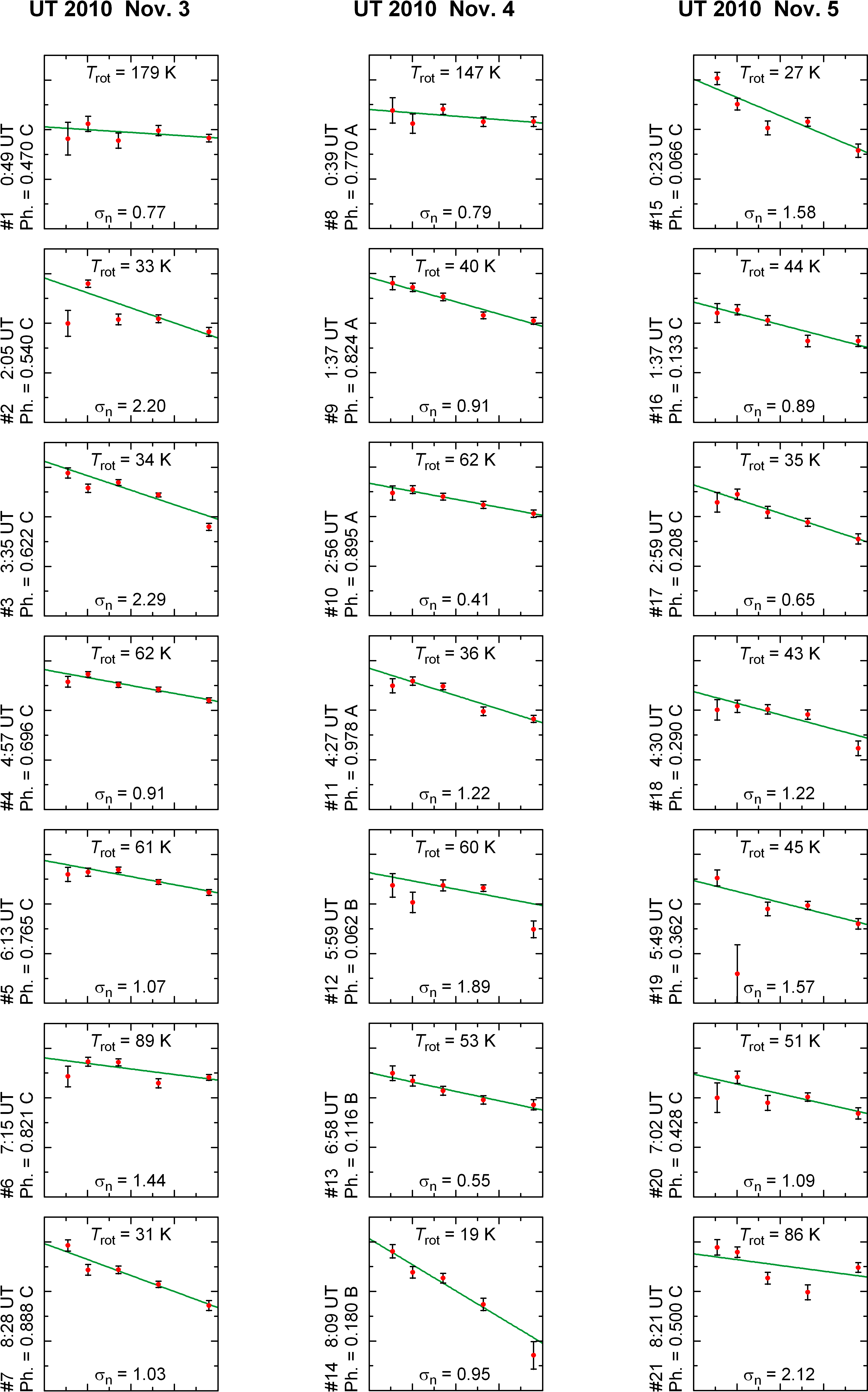
Figure 12: Full set of the 21 rotational diagrams derived from the time series of CH₃OH, with weighted linear least-squares fits. Other details, including the description of the figure axes, are the same as in Fig. 3. This material is also contained in Animation 1.

This appendix contains the complete material used in this work. In Table 2 we show the time series of all line parameters and corresponding physical quantities, while Figs. 12 and 13 contain all the rotational diagrams and line profiles, respectively.

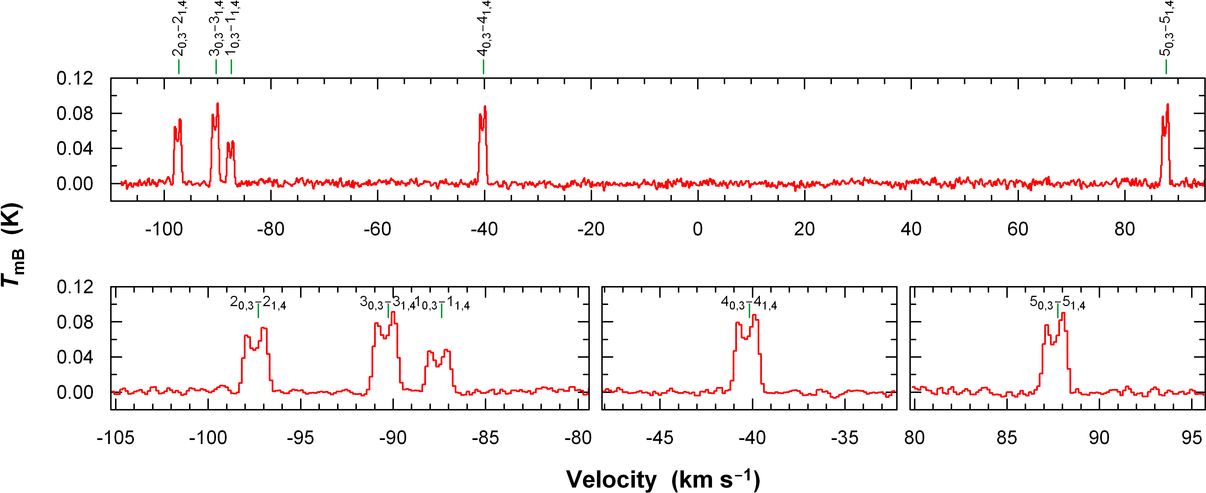
Figure 1: Mean spectrum of CH₃OH resulting from all 21 spectra in our time series. The zero velocity corresponds to the rest frequency of 157.225 GHz. The transitions are labeled and the rest velocities are indicated by the short vertical lines. The top panel shows the full spectrum whereas the bottom panels show close-up views of the line profiles.

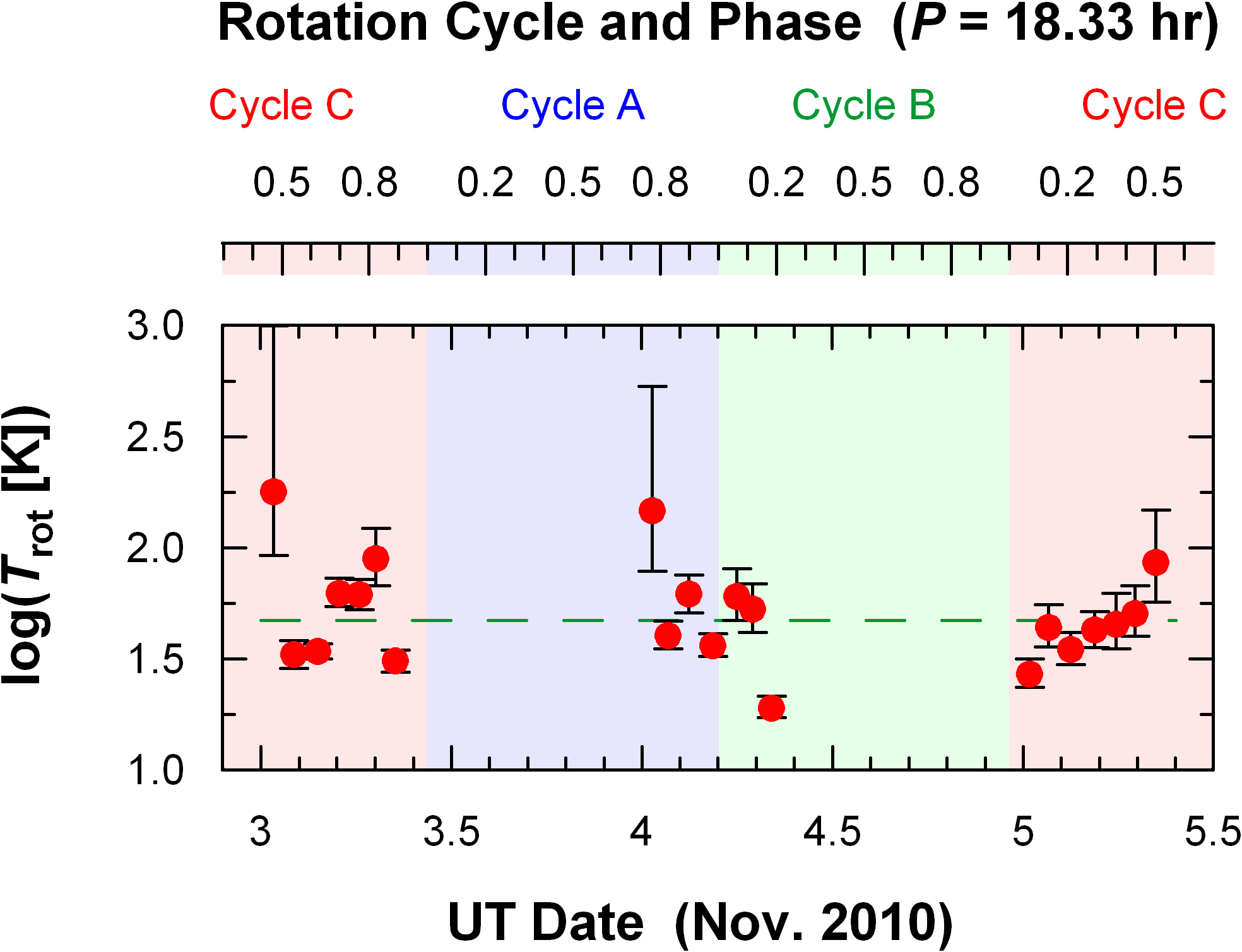
Figure 4: Variation of the logarithmic rotational temperature $\log(T_{\mathrm{rot}})$ with time, derived from the time series of CH₃OH. The dashed line indicates the temperature level of 47 K obtained from the mean spectrum (Figs. 1 and 6). The additional top axis shows the nucleus rotation phase and three-cycle component (cf. Paper I), and the latter is also coded by the background color. The EPOXI flyby occurred on UT 2010 Nov. 4.5832, corresponding to phase 0.5 of Cycle B.

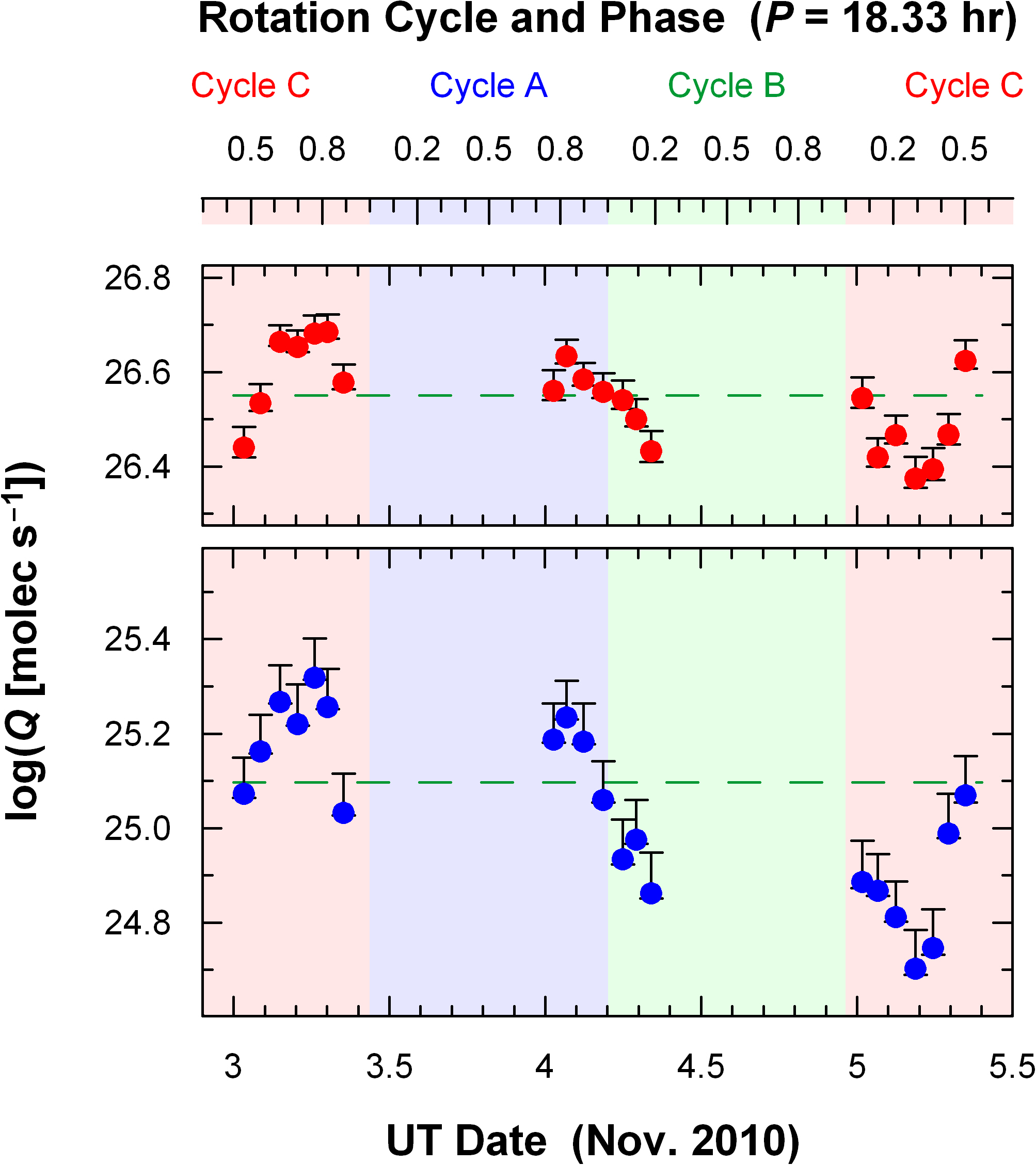
Figure 8: Production-rate variability in CH₃OH (top panel) and HCN (bottom panel) presented in logarithmic scale. The production rates $Q$ vary about the average values: $3.5\times 10^{26}$ molec s^-1 for CH₃OH and $1.25\times 10^{25}$ molec s^-1 for HCN (dashed lines). The asymmetry of the error bars results from the uncertainty of the telescope pointing (cf. Paper I), which surpasses the errors from noise. For this reason, the uncertainties on the simultaneous measurements of CH₃OH and HCN are partly correlated, unlike the errors on subsequent data points. Systematic errors affecting only the absolute levels were neglected (cf. Section 2) as they do not change the shapes of the variability profiles. The additional top axis shows the nucleus rotation phase and three-cycle component (cf. Paper I), and the latter is also coded by the background color. The EPOXI flyby occurred on UT 2010 Nov. 4.5832, corresponding to phase 0.5 of Cycle B.

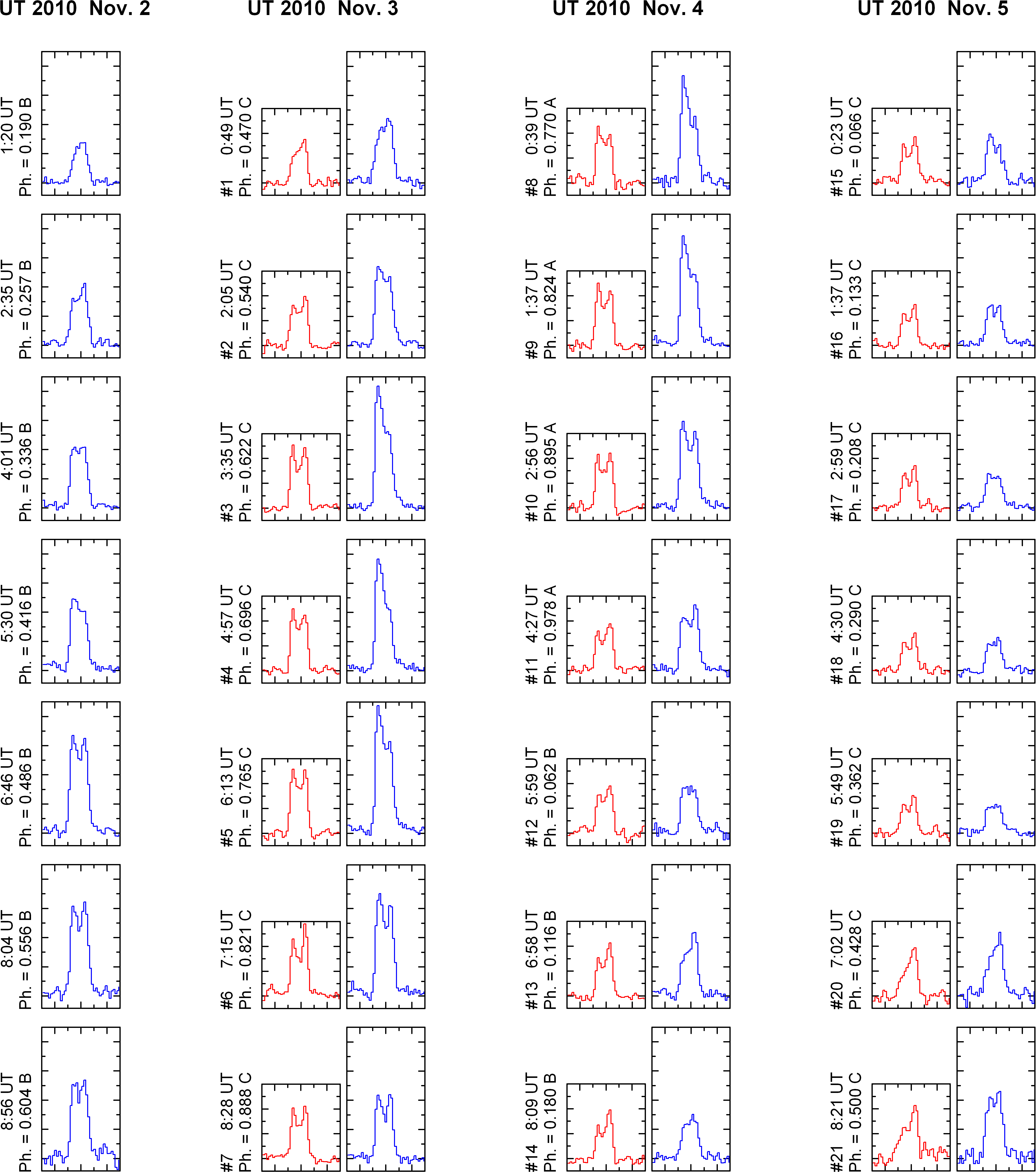
Figure 13: Full set of the 28 line profiles of HCN (blue) and 21 line profiles of CH₃OH (red) illustrating the temporal variations. Other details, including the description of the figure axes, are the same as in Fig. 10. This material is also contained in Animation 2.

Table 1: Transition and Telescope Constants

Molecule	Transition	$\nu_{ul}$	$A_{ul}$	$g_{u}$	$E_{u}/k$	Beam		$\tau_{\perp}$	$\Delta v$	$\eta_{\mathrm{mB}}$
		(GHz)	($10^{-6}$ s-1)		(K)	(″)	(km)	(min)	(m s-1)
HCN	J(3–2)	265.886434	835.55	21	25.521	4.4	495	10.3	044	0.52
CH3OH	$5_{0,3}$–$5_{1,4}$	157.178987	020.38	11	47.936	7.4	826	17.2	149	0.72
	$4_{0,3}$–$4_{1,4}$	157.246062	020.98	09	36.335
	$1_{0,3}$–$1_{1,4}$	157.270832	022.06	03	15.447
	$3_{0,3}$–$3_{1,4}$	157.272338	021.46	07	27.053
	$2_{0,3}$–$2_{1,4}$	157.276019	021.82	05	20.090

Note. — Molecular constants for CH₃OH are taken from the Pearson & Xu (2010) update to the JPL Molecular Catalog (Pickett et al., 1998), available online at http://spec.jpl.nasa.gov, whereas the constants for HCN are from the Cologne Database for Molecular Spectroscopy (Müller et al., 2005), available at http://www.astro.uni-koeln.de/cdms.

Table 2: Complete Time Series of the Line Parameters and Corresponding Physical Quantities

#	UT Date	$\Delta\mathrm{t}$	Phase	CH3OH				HCN
	(Nov. 2010)	(min)	& Cycle	$\int\!\!T_{\mathrm{mB}}\mathrm{d}v$	$v_{0}$	$T_{\mathrm{rot}}$	$\log(Q)$	$\int\!\!T_{\mathrm{mB}}\mathrm{d}v$	$v_{0}$	$\log(Q)$
	$2.0558$	$51.2$	0.190 B	$\cdots$	$\cdots$	$\cdots$	$\cdots$	$0.672_{-0.021}^{+0.106}$	$-0.002_{-0.022}^{+0.023}$	$24.813_{-0.013}^{+0.081}$
	$2.1075$	$61.3$	0.257 B	$\cdots$	$\cdots$	$\cdots$	$\cdots$	$1.060_{-0.017}^{+0.164}$	$-0.032_{-0.014}^{+0.014}$	$25.011_{-0.007}^{+0.078}$
	$2.1672$	$61.9$	0.336 B	$\cdots$	$\cdots$	$\cdots$	$\cdots$	$1.234_{-0.012}^{+0.190}$	$-0.117_{-0.012}^{+0.011}$	$25.076_{-0.004}^{+0.078}$
	$2.2289$	$61.6$	0.416 B	$\cdots$	$\cdots$	$\cdots$	$\cdots$	$1.357_{-0.013}^{+0.219}$	$-0.180_{-0.013}^{+0.012}$	$25.118_{-0.004}^{+0.082}$
	$2.2817$	$61.0$	0.486 B	$\cdots$	$\cdots$	$\cdots$	$\cdots$	$1.890_{-0.020}^{+0.290}$	$-0.120_{-0.011}^{+0.011}$	$25.262_{-0.004}^{+0.077}$
	$2.3359$	$60.4$	0.556 B	$\cdots$	$\cdots$	$\cdots$	$\cdots$	$1.786_{-0.031}^{+0.285}$	$-0.068_{-0.020}^{+0.022}$	$25.237_{-0.007}^{+0.081}$
	$2.3723$	$20.7$	0.604 B	$\cdots$	$\cdots$	$\cdots$	$\cdots$	$1.509_{-0.041}^{+0.257}$	$-0.049_{-0.029}^{+0.032}$	$25.164_{-0.012}^{+0.087}$
0$1$	$3.0339$	$61.1$	0.470 C	$0.070_{-0.003}^{+0.007}$	$-0.043_{-0.034}^{+0.037}$	$179_{-86}^{+816}$	$26.440_{-0.020}^{+0.044}$	$1.222_{-0.024}^{+0.186}$	$-0.033_{-0.014}^{+0.013}$	$25.072_{-0.008}^{+0.077}$
0$2$	$3.0868$	$61.9$	0.540 C	$0.088_{-0.003}^{+0.007}$	$-0.091_{-0.035}^{+0.035}$	$33_{-4}^{+5}$	$26.534_{-0.017}^{+0.040}$	$1.503_{-0.016}^{+0.232}$	$-0.152_{-0.011}^{+0.011}$	$25.162_{-0.005}^{+0.079}$
0$3$	$3.1495$	$61.5$	0.622 C	$0.118_{-0.002}^{+0.009}$	$-0.114_{-0.026}^{+0.026}$	$34_{-3}^{+3}$	$26.664_{-0.009}^{+0.035}$	$1.916_{-0.017}^{+0.296}$	$-0.249_{-0.008}^{+0.008}$	$25.268_{-0.004}^{+0.078}$
0$4$	$3.2062$	$61.7$	0.696 C	$0.115_{-0.003}^{+0.009}$	$-0.135_{-0.024}^{+0.022}$	$62_{-8}^{+11}$	$26.653_{-0.011}^{+0.036}$	$1.720_{-0.014}^{+0.282}$	$-0.263_{-0.007}^{+0.008}$	$25.221_{-0.004}^{+0.084}$
0$5$	$3.2593$	$61.7$	0.765 C	$0.123_{-0.003}^{+0.010}$	$-0.168_{-0.027}^{+0.027}$	$61_{-9}^{+11}$	$26.681_{-0.012}^{+0.038}$	$2.154_{-0.019}^{+0.343}$	$-0.171_{-0.008}^{+0.009}$	$25.319_{-0.004}^{+0.083}$
0$6$	$3.3020$	$30.2$	0.821 C	$0.124_{-0.004}^{+0.010}$	$-0.037_{-0.046}^{+0.044}$	$89_{-22}^{+32}$	$26.685_{-0.014}^{+0.037}$	$1.869_{-0.021}^{+0.293}$	$-0.085_{-0.013}^{+0.013}$	$25.257_{-0.005}^{+0.080}$
0$7$	$3.3527$	$74.9$	0.888 C	$0.097_{-0.003}^{+0.008}$	$-0.152_{-0.036}^{+0.039}$	$31_{-3}^{+4}$	$26.578_{-0.015}^{+0.037}$	$1.115_{-0.013}^{+0.180}$	$-0.124_{-0.022}^{+0.021}$	$25.032_{-0.005}^{+0.082}$
0$8$	$4.0268$	$30.0$	0.770 A	$0.093_{-0.004}^{+0.009}$	$-0.224_{-0.042}^{+0.037}$	$147_{-69}^{+385}$	$26.560_{-0.020}^{+0.045}$	$1.595_{-0.028}^{+0.243}$	$-0.235_{-0.014}^{+0.014}$	$25.188_{-0.007}^{+0.077}$
0$9$	$4.0676$	$60.5$	0.824 A	$0.110_{-0.004}^{+0.008}$	$-0.176_{-0.034}^{+0.035}$	$40_{-5}^{+6}$	$26.633_{-0.015}^{+0.036}$	$1.775_{-0.019}^{+0.271}$	$-0.215_{-0.009}^{+0.010}$	$25.234_{-0.005}^{+0.077}$
$10$	$4.1222$	$61.3$	0.895 A	$0.098_{-0.003}^{+0.007}$	$-0.165_{-0.029}^{+0.029}$	$62_{-11}^{+14}$	$26.584_{-0.013}^{+0.035}$	$1.577_{-0.017}^{+0.250}$	$-0.124_{-0.012}^{+0.011}$	$25.183_{-0.005}^{+0.081}$
$11$	$4.1852$	$61.3$	0.978 A	$0.093_{-0.003}^{+0.008}$	$-0.059_{-0.031}^{+0.038}$	$36_{-4}^{+5}$	$26.559_{-0.014}^{+0.039}$	$1.186_{-0.015}^{+0.191}$	$-0.026_{-0.016}^{+0.018}$	$25.059_{-0.005}^{+0.083}$
$12$	$4.2492$	$30.3$	0.062 B	$0.089_{-0.004}^{+0.008}$	$-0.114_{-0.044}^{+0.048}$	$60_{-13}^{+20}$	$26.541_{-0.019}^{+0.041}$	$0.889_{-0.021}^{+0.146}$	$-0.082_{-0.024}^{+0.025}$	$24.934_{-0.010}^{+0.085}$
$13$	$4.2904$	$60.8$	0.116 B	$0.081_{-0.003}^{+0.007}$	$+0.017_{-0.035}^{+0.034}$	$53_{-11}^{+16}$	$26.500_{-0.016}^{+0.043}$	$0.978_{-0.020}^{+0.160}$	$+0.020_{-0.020}^{+0.020}$	$24.976_{-0.009}^{+0.085}$
$14$	$4.3399$	$60.4$	0.180 B	$0.069_{-0.004}^{+0.006}$	$-0.007_{-0.043}^{+0.044}$	$19_{-2}^{+3}$	$26.432_{-0.023}^{+0.043}$	$0.753_{-0.019}^{+0.125}$	$-0.004_{-0.024}^{+0.023}$	$24.862_{-0.011}^{+0.087}$
$15$	$5.0163$	$60.5$	0.066 C	$0.090_{-0.004}^{+0.008}$	$+0.006_{-0.052}^{+0.056}$	$27_{-3}^{+5}$	$26.545_{-0.021}^{+0.043}$	$0.795_{-0.024}^{+0.135}$	$-0.225_{-0.033}^{+0.026}$	$24.886_{-0.013}^{+0.088}$
$16$	$5.0673$	$60.3$	0.133 C	$0.067_{-0.003}^{+0.006}$	$-0.078_{-0.039}^{+0.044}$	$44_{-8}^{+12}$	$26.420_{-0.020}^{+0.041}$	$0.762_{-0.019}^{+0.117}$	$-0.123_{-0.029}^{+0.026}$	$24.867_{-0.011}^{+0.078}$
$17$	$5.1246$	$61.4$	0.208 C	$0.075_{-0.003}^{+0.006}$	$-0.057_{-0.051}^{+0.055}$	$35_{-5}^{+7}$	$26.467_{-0.019}^{+0.040}$	$0.670_{-0.013}^{+0.101}$	$-0.147_{-0.023}^{+0.025}$	$24.811_{-0.009}^{+0.076}$
$18$	$5.1873$	$61.3$	0.290 C	$0.061_{-0.003}^{+0.006}$	$-0.065_{-0.050}^{+0.051}$	$43_{-7}^{+9}$	$26.375_{-0.021}^{+0.046}$	$0.521_{-0.016}^{+0.084}$	$-0.044_{-0.028}^{+0.030}$	$24.702_{-0.013}^{+0.082}$
$19$	$5.2426$	$61.3$	0.362 C	$0.063_{-0.003}^{+0.006}$	$-0.076_{-0.044}^{+0.060}$	$45_{-10}^{+17}$	$26.394_{-0.022}^{+0.045}$	$0.578_{-0.021}^{+0.092}$	$-0.083_{-0.033}^{+0.034}$	$24.747_{-0.015}^{+0.081}$
$20$	$5.2932$	$60.8$	0.428 C	$0.075_{-0.004}^{+0.007}$	$+0.004_{-0.034}^{+0.033}$	$51_{-11}^{+17}$	$26.467_{-0.021}^{+0.043}$	$1.009_{-0.022}^{+0.165}$	$+0.028_{-0.024}^{+0.025}$	$24.989_{-0.009}^{+0.084}$
$21$	$5.3477$	$60.3$	0.500 C	$0.107_{-0.004}^{+0.010}$	$+0.074_{-0.040}^{+0.049}$	$86_{-29}^{+62}$	$26.623_{-0.016}^{+0.044}$	$1.216_{-0.044}^{+0.197}$	$-0.042_{-0.031}^{+0.034}$	$25.070_{-0.015}^{+0.083}$

Note. — $\Delta\mathrm{t}$ is the time coverage of the measurement; other symbols and units are the same as defined and used throughout the paper. The errors on $\int\!\!T_{\mathrm{mB}}\mathrm{d}v$ and on the resulting $Q$ include the uncertainty of the telescope pointing, and therefore are partly correlated in the simultaneous measurements of CH₃OH and HCN, unlike the errors on subsequent data points. The errors on $v_{0}$ and $T_{\mathrm{rot}}$ are free of the pointing contribution and therefore are fully independent, both in time and between the molecules.

References

- A’Hearn (2011) A’Hearn, M. F., 2011, EPSC Abstracts, 6, 316
- A’Hearn et al. (2011) A’Hearn, M. F., et al., 2011, Science, 332, 1396
- Biver et al. (2002a) Biver, N., et al., 2002a, EM&P, 90, 5
- Biver et al. (2002b) Biver, N., et al., 2002b, EM&P, 90, 323
- Biver et al. (2007) Biver, N., et al., 2007, Icarus, 187, 253
- Bockelée-Morvan et al. (1984) Bockelée-Morvan, D., et al., 1984, A&A, 141, 411
- Bockelée-Morvan et al. (1994) Bockelée-Morvan, D., Crovisier, J., Colom, P., Despois, D., 1994, A&A, 287, 647
- Combi et al. (2004) Combi, M. R., Harris, W. M., Smyth, W. H., 2004, in Comets II, eds. M. C. Festou, H. U. Keller, H. A. Weaver (Tucson: Univ. of Arizona Press), 523
- Combi et al. (2011) Combi, M. R., Bertaux, J.-L., Quémerais, E., Ferron, S., Mäkinen, J. T. T., 2011, ApJ, 734, L6
- Dello Russo et al. (2007) Dello Russo, N., et al., 2007, Nature, 448, 172
- Dello Russo et al. (2011) Dello Russo, N., et al., 2011, ApJ, 734, L8
- Dones et al. (2004) Dones, L., Weissman, P. R., Levison, H. F., Duncan, M. J., 2004, in Comets II, eds. M. C. Festou, H. U. Keller, H. A. Weaver (Tucson: Univ. of Arizona Press), 153
- Drahus (2009) Drahus, M., 2009, Microwave observations and modeling of the molecular coma in comets, Ph. D. thesis (Univ. of Göttingen)
- Drahus et al. (2010) Drahus, M., et al., 2010, A&A, 510, A55
- Drahus et al. (2011) Drahus, M., et al., 2011, ApJ, 734, L4
- Duncan et al. (2004) Duncan, M., Levison, H., Dones, L., 2004, in Comets II, eds. M. C. Festou, H. U. Keller, H. A. Weaver (Tucson: Univ. of Arizona Press), 193
- Feaga et al. (2007) Feaga, L. M., A’Hearn, M. F., Sunshine, J. M., Groussin, O., Farnham, T. L., 2007, Icarus, 191, 134
- Gibb et al. (2007) Gibb, E. L., et al., 2007, Icarus, 188, 224
- Giorgini et al. (1997) Giorgini, J. D., et al., 1997, BAAS, 28, 1099
- Guilbert-Lepoutre & Jewitt (2011) Guilbert-Lepoutre, A., Jewitt, D., 2011, ApJ, 743, 31
- Harmon et al. (2011) Harmon, J. K., Nolan, M. C., Howell, E. S., Giorgini, J. D., Taylor, P. A., 2011, ApJ, 734, L2
- Hartley (1986) Hartley, M., 1986, IAU Circ., 4197
- Huebner et al. (1992) Huebner, W. F., Keady, J. J., Lyon, S. P., 1992, Ap&SS, 195, 1
- Knight & Schleicher (2011) Knight, M. M., Schleicher, D. G., 2011, AJ, 141, 183
- Kramer (1997) Kramer, C., 1997, Calibration of spectral line data at the IRAM 30m radio telescope, IRAM Report
- Levison (1996) Levison, H. F., 1996, ASP Conf., 107, 173
- Levison et al. (2010) Levison, H. F., Duncan, M. J., Brasser, R., Kaufmann, D. E., 2010, Science, 329, 187
- Mumma et al. (2011) Mumma, M. J., et al., 2011, ApJ, 734, L7
- Müller et al. (2005) Müller, H. S. P., Schlöder, F., Stutzki, J., Winnewisser, G., 2005, J. Mol. Struct., 742, 215
- Pearson & Xu (2010) Pearson, J. C., Xu, L.-H, 2010, in JPL Molecular Catalog
- Pickett et al. (1998) Pickett, H. M., et al., 1998, J. Quant. Spec. Radiat. Transf., 60, 883
- Prialnik et al. (2004) Prialnik, D., Benkhoff, J., Podolak, M., 2004, in Comets II, eds. M. C. Festou, H. U. Keller, H. A. Weaver (Tucson: Univ. of Arizona Press), 359
- Samarasinha et al. (2011) Samarasinha, N. H., Mueller, B. E. A., A’Hearn, M. F., Farnham, T. L., Gersch, A., 2011, ApJ, 734, L3
- Ulich & Haas (1976) Ulich, B. L., Haas, R. W., 1976, ApJS, 30, 247
- Villanueva et al. (2012) Villanueva, G. L., DiSanti, M. A., Mumma, M. J., Xu, L.-H., 2012, ApJ, 747, 37
- Waniak et al. (2012) Waniak, W., Borisov, G., Drahus, M., Bonev, T., 2012, A&A, 543, A32
- Weidenschilling (1977) Weidenschilling, S. J., 1977, MNRAS, 180, 57
- Yamamoto (1985) Yamamoto, T., 1985, A&A, 142, 31