Variability in X-ray line ratios in helium-like ions of massive stars: the radiation-driven case

Abstract

Context. Line ratios in “$fir$” triplets of helium-like ions have proven to be a powerful diagnostic of conditions in X-ray emitting gas surrounding massive stars. Recent observations indicate that these ratios can be variable with time.

Aims. The possibilities for causes of variation in line $ratios$ are limited: changes in the radiation field or changes in density, which would result in radiational or collisional level-pumping, respectively; and changes in mass-loss or geometry, which could cause variations in X-ray absorption effects. In this paper, we explore the first of these potential causes of variability: changes in the radiation field. We therefore explore the conditions necessary to induce variability in the ratio $R=f/i$ via this mechanism.

Methods. To isolate the radiative effect, we use a heuristic model of temperature and radius changes in variable stars in the B and O range with low-density, steady-state winds. We then model the changes in emissivity of X-ray emitting gas close to the star due to differences in level-pumping owing to the availability of UV photons at the location of the gas.

Results. We find that under these conditions, variability in $R$ is dominated by the stellar temperature. Although the relative amplitude of variability is roughly comparable for most lines at most temperatures, detectable variations are limited to a few lines for each spectral type. We predict that variable values in $R$ due to stellar variability must follow predictable trends found in our simulations.

Conclusions. Our heuristic model uses radial pulsations as a mode of stellar variability that maximizes the amplitude of variation in $R$. This model is robust enough to provide a guide to which ions will provide the best opportunity for observing variability in the $f/i$ ratio at different stellar temperatures, and the correlation of that variability with other observable parameters. In real systems, however, the effects would be more complex than in our model, with differences in phase and suppressed amplitude in the presence of non-radial pulsations. This, combined with the range of amplitudes produced in our simulations, suggest that changes in $R$ across many lines concurrently are not likely to be produced by a variable radiation field.

1 Introduction

Astrophysical studies at X-ray wavelengths have been revolutionized through high resolution spectroscopy afforded by the Chandra and XMM-Newton telescopes. Diagnostics for temperature, density, flow dynamics, and geometry can be observed with these telescopes through the use of resolved spectral lines from X-ray emitting plasmas. Our understanding of massive star winds in particular has been impacted by these new observational capabilities.

With the large investment of observing time in existing studies of hot plasma emissions from massive stars, we believe that the next natural step in understanding these X-ray sources is to consider their spectral variability. This is in many ways a fledgling field, since substantial amounts of observing time is required merely to resolve lines. Still, some sources such as $\zeta$ Pup have been observed in excess of 1 Msec over a period of many years. The fast winds of massive stars have a flow time given by the ratio of the stellar radius $r_{\star}$ to the wind terminal speed $v_{\infty}$, with $r_{\star}/v_{\infty}\sim$ ksec timescales. Many of these stars also have rotation speeds of hundreds of ${\rm km\leavevmode\nobreak\ s^{-1}}$, implying rotational periods of days to weeks, on order of a Msec. Thus there is good physical motivation to investigate X-ray variability for these sources at these timescales.

There have already been several observational studies of X-ray variability among massive star sources. Some examples include colliding wind binaries (e.g., $\eta$ Car: Henley et al. 2008, Corcoran et al. 2001, Leutenegger et al. 2003; $\gamma$ Vel: Skinner et al. 2001, Henley et al. 2005, Schild et al. 2004, Stevens et al. 1996; WR 140: Pollock et al. 2005; WR 147: Zhekov & Park 2010, Skinner et al. 2007), mass transfer binaries (e.g., $\beta$ Lyr: Ignace et al. 2008), magnetic stars (e.g., $\theta^{1}$ Ori C: Gagne et al. 2005; Ignace et al. 2010; $\sigma$ Ori E: Groote & Schmitt 2004; $\tau$ Sco: Ignace et al. 2010, Mewe et al. 2003b, Cohen et al. 2003), or pulsator stars (e.g., Favata et al. 2009; Oskinova et al. in press). These sources tend to be unusual in some manner such that cyclical variability is to be expected. Some variability studies have also targeted nominally single stars (e.g., $\zeta$ Pup: Berghoefer et al. 1996; WR 46: Gosset et al. 2011).

Although not true in every case, many of these variability studies have been limited to considerations of X-ray passband variability or variability of low resolution spectral energy distributions (SEDs). There have been some exceptions, however, notably the work of Henley et al. (2008) on $\eta$ Car or the Favata et al. (2009) data set on $\beta$ Cep, in which variations are seen in some individual emission lines.

New reports of spectral line variability are emerging, such as that by Nichols et al. (2011), who analyzed archival data for a number of massive star sources, and a study of $\kappa$ Ori by Waldron et al. (priv. comm.). Although the data are not yet adequate to conduct a full period analysis, it does appear that the $R$ ratio (discussed below) has detectable variations in several helium-like ions at the same time from putatively-single massive stars. As a ratio involving components from a line triplet, such variations cannot simply arise as a result of emission measure (EM) variations. Instead, they are sensitive to other important effects that provide fresh diagnostic value for understanding massive star X-ray emission processes. While these reports of line variability are still undergoing analysis, it does seem timely to engage in a discussion of the theoretical expectations for line variability.

While there are many possibilities for the causes of such variability, in this first contribution we limit the scope of our discussion to how the triplet lines of He-like species can vary in response to a changing radiation field. These X-ray lines, which include the forbidden, intercombination, and resonance (“$fir$”) triplets of abundant metal species such as N vi, O vii, Ne ix and so on, are typically quite strong. There is a fairly broad range of X-ray temperatures in which these species can be the dominant stage of ionization (e.g., Cox 2000). Thus the triplet lines have long been used as important diagnostics of the hot plasma.

Gabriel & Jordan (1969) discussed two key line ratios that could be formed from the triplet. The first was a ratio of the forbidden line emission to that of the intercombination line, with $R=f/i$. The second involved a ratio of the sum of the $f$ and $i$ line components to that of the resonance line $r$, with $G=(f+i)/r$. Under the condition of collisionally dominated excitation, the ratio $G$ is sensitive to plasma temperature, whereas the ratio $R$ is sensitive to pumping processes that can depopulate the $f$ level to the $i$ level. Blumenthal et al. (1972) continued the work by Gabriel & Jordan, clarifying the concepts and emphasizing the sensitivity of $R$ to the radiation field.

It is the radiative pumping that has proven to be of tremendous diagnostic value in applications to massive stars (e.g. Kahn et al. 2001; Waldron & Cassinelli 2001). Pumping for the most common X-ray lines occurs in the UV, where massive stars have peak brightnesses. In these stars, X-ray emissions can be produced in the wind outflow, owing to the formation of highly supersonic shocks arising from a natural instability in the line-driving mechanism that accounts for the wind acceleration (e.g., Lucy 1982; Owocki et al. 1988; Feldmeier et al. 1997; Dessart & Owocki 2003). Since the X-ray emissions are distributed above the photosphere, radiative pumping is also a function of radius via the dilution factor, because the pumping rate depends on the mean intensity of radiation. As a result, the $R$ ratio has been employed as a means of determining or limiting the location of X-ray sources in the circumstellar environment of massive stars.

Here we focus specifically on the $R$ ratio for a circumstellar source of X-ray emission around a UV bright star. There are essentially four things that can modify line emissions in the regime of collisional ionization equilibrium (CIE): density variations that affect the scale of the EM; density variations that affect collisional pumping between the levels; variations of the radiation field that affect the radiative pumping between levels; and variations in the hot plasma temperature. Of these, the first two will not influence the ratios $G$ and $R$, because variations in EM for optically thin lines is a simple scaling factor that will cancel in the ratio. The $R$ ratio is sensitive to pumping effects, but $G$ is largely insensitive; on the other hand $G$ is temperature sensitive, whereas $R$ is less sensitive to this parameter. Thus here we are mostly concerned with variations in the stellar radiation field at specific line pumping wavelengths.

Our goal is to develop a model that will produce the most general results possible. To this end, we seek to maximize the amplitude of variability from our model. In other words we seek to develop a model that is as optimistic as possible for detecting variable ratios of $R$. We therefore consider a phenomenological model of a B star or O star that is a simple radial pulsator (see Sect. 2.2). The star is assumed to have a low mass-loss rate ($\dot{M}$, which allows us to ignore both photoabsorption of X-ray emissions by the wind itself and collisional pumping effects. This model has the potential to affect the $R$ ratio in two ways. First, variations in stellar temperature $T_{\star}$ will change the shape and intensity of the blackbody radiation around the star. Second, changes in stellar photospheric radius $r_{\star}$ can impact the dilution factor at the location of the emitter.

A “toy” pulsating star model for influencing X-ray emission lines is presented in Sect. 2. Results of our simulations are presented in terms of a parameter study in Sect. 3. A discussion of applications to massive stars follows in Sect. 4, including a qualitative discussion of expectations when assumptions of the current model are relaxed.

2 Model

2.1 Radiative equations

The total line emission from the triplet components are described in terms of luminosities, $L_{f}$, $L_{i}$, and $L_{r}$ (or $f$, $i$, and $r$) representing the line luminosities, respectively. The $R$ ratio is then:

$$R=\frac{L_{f}}{L_{i}}.$$ (1)

Blumenthal et al. (1972) showed that in a hot plasma this ratio goes as

$$R=\frac{R_{0}}{1+\phi_{\nu}/\phi_{\rm c}+n_{\rm e}/n_{\rm c}},$$ (2)

where $\phi_{\nu}$ is the intensity of radiation at the frequency corresponding to the transition between the $i$ and $f$ energy levels for a given helium-like ion; $n_{\rm e}$ is the electron density; and $R_{0}$, $\phi_{\rm c}$ and $n_{\rm c}$ are determined by atomic parameters and the electron temperature of the emitting gas. The value of $R_{0}$ is a weak function of temperature under the conditions of CIE (Blumenthal et al. 1972), which are generally thought to hold for massive star X-ray emissions. Atomic constants for a number of common ions used in our simulations are listed in Table 1.

Table 1: Physical constants for six He-like ions used in our simulations.

Line	$\lambda_{\rm f}$ a	$\lambda_{\rm i}$ a	$\lambda_{\rm r}$ a	$A_{\rm if}$ b	$\phi_{\rm c}$ b	$F$ b
	(Å)	(Å)	(Å)	(s-1)	(s-1)
C v	41.46	40.71	40.28	1.14$\times 10^{8}$	3.57$\times 10^{1}$	0.36
N vi	29.53	29.08	28.79	1.37$\times 10^{8}$	1.83$\times 10^{2}$	0.38
O vii	22.10	21.80	21.60	1.61$\times 10^{8}$	7.32$\times 10^{2}$	0.42
Ne ix	13.70	13.55	13.45	2.12$\times 10^{8}$	7.73$\times 10^{3}$	0.41
Mg xi	9.31	9.23	9.17	2.68$\times 10^{8}$	4.86$\times 10^{4}$	0.49
Si xiii	6.74	6.69	6.65	3.32$\times 10^{8}$	2.39$\times 10^{5}$	0.49

(a) Porquet et al. (2001); (b) Blumenthal et al. (1972).

Since our intention is to investigate how a change in the stellar radiation field affects $R$, in our simulations we may safely assume $n_{\rm e}\ll n_{\rm c}$ for B star winds, as discussed in the previous section. The radiative pumping rate $\phi$ (in units of photons s^-1) is defined as

$$\phi=A_{tot}W\left[e^{\beta}-1\right]^{-1},$$ (3)

where $A_{tot}$ is the sum of the three Einstein A-coefficients for the transition between the $i$ and $f$ energy levels, $\beta=h\nu/k_{B}T_{\star}$ (with $T_{\star}$ the time-dependent stellar effective temperature producing a blackbody radiation field), and $W(r)$ is the geometrical dilution factor for the intensity of the stellar radiation field at the location of the gas. In our simulations, we follow Blumenthal et al. in using $A_{tot}=3A_{\rm if}$, with values of $A_{\rm if}$ listed in Table 1. For a star without limb darkening, and ignoring any diffuse radiation field in the wind itself, the dilution factor is a simple function of radius given by

$$W=\frac{1}{2}\left[1-\sqrt{1-\left(\frac{r_{\star}}{r}\right)^{2}}\right]$$ (4)

One should bear in mind some of the limitations implied by our restrictive model. For example, a hot gas component arising from a shock in a wind, or from confined flow in a magnetosphere, will have a range of temperatures. Having a range of temperatures would create a distribution of $R_{0}$ values within the gas, as well as changing the ionization fraction. If $R_{0}$ varies spatially within the gas, the differing values of $R$ will tend to dampen the variation of $R$ with the radiation field, making it harder to detect. If ionization is allowed to change with stellar temperature, that adds another potentially confounding variable that would making it more difficult to observe the variation.

The above-mentioned effects could be considered; however, their inclusion would require us to choose a particular dependence of the temperature of the X-ray emitting gas ($T_{X}$)with radius, making the results model dependent. In these simulations we omit such considerations and follow Blumenthal et al. (1972) in using the $R_{0}$ of each ion at the temperature where it will have the maximum signal. This would seem to imply physically not only that we have a multi-temperature gas, but one in which each element had a different temperature. However, since the emissivity of each ion is a fairly sharp function of temperature, while $R_{0}$ is a weak function of $T$, this is a reasonable approximation of the response of the gas. Here it is worth stressing again that there are many ways in which variability in $R$ may be suppressed, and that our simple model is an attempt to find the most optimistic approach for how the stellar radiation field could drive an observable variation in the value of $R$. We address expansions of our results to more generalized cases in Sect. 4.

2.2 System model

We have chosen to use B stars as the basis for our models. B stars have sufficient UV fields to cause radiative pumping, are hot enough to produce the necessary X-ray emission, yet have low enough mass-loss that we can avoid complications of density-induced collisional level pumping as well as photoabsorption of X-rays within the wind. We also extend our models to higher, O star temperatures with the constraint that their mass-loss remains low. This should be kept in mind when interpreting our results for early-type stars.

Although variable early-type stars (e.g., $\beta$ Cepheids) are non-radial pulsators, our “toy” radial pulsator has the advantage of maximizing the amplitude (and thus observability) of variation in $R$. This is because in radial pulsations, the entire surface of the star changes in brightness, temperature and position in the same sense (i.e. brighter or dimmer) at the same time, whereas a non-radial pulsator has some parts that are changing in opposing ways at the same time. Thus we model radial pulsations in our stars so that our calculations will produce upper limits to variations of $R$.

We consider a range of stellar parameters appropriate for B and low-$\dot{M}$ O stars: radii of 1.8 to 11.0 $r_{\sun}$ and effective surface temperatures in the range 10,000 to 40,000 K. For simplicity, the radiation field is assumed to follow a blackbody curve. Radius and temperature variations with amplitudes of 10-20% are considered, typical of radially-pulsating classical Cepheid stars (e.g., Bono et al. 2000). We adopt simple sinusoidal forms for the radius and temprature evolution in angular pulsational phase $\xi$, with:

$$T_{\star}(t)=T_{0}\left[1+\Delta T\cos{\left(\xi-\psi\right)}\right],$$ (5)

$$r_{\star}(t)=r_{\star,0}\left[1+\Delta r_{\star}\cos{\xi}\right].$$ (6)

Stellar pulsations, such as those caused by the $\kappa$-mechanism, generally have a phase offset between changes in the radius and in the effective temperature of the star. Our model allows for such an offset by varying $\psi$. Note that actual pulsations tend to have waveforms that are more complex than a sinusoidal function; however, our general conclusions do not depend on such details, and calculations can be modified to allow for any specific waveform desired.

Table 2: Simulation parameters for the stellar system.

$T_{\star,0}$	$\Delta$T	$r_{\star,0}$	$\Delta r$	$r_{\rm gas}$
(K)	($T_{\star,0}$)	($r_{\sun}$)	($r_{\star}$)	($r_{\sun}$)
10,000	0.20	1.8	0.20	3.6
20,000	0.15	4.0	0.15	8.0
30,000	0.10	6.5	0.10	13.0
40,000	0.10	11.0	0.10	22.0

In our model, the hot X-ray emitting gas is placed approximately 1 $r_{\star}$ above the surface of the star (i.e., $r_{\rm gas}=2r_{\star}$; see Fig. 1). This hot zone is to be considered as a “test particle” for our calculations. A change in temperature drives a change in the UV hardness of the radiation field with time and thus the pumping of the $f$ level; a change in location of the hot zone modifies the dilution factor $W(r)$ and consequently the pumping owing to the mean intensity. If the hot zone moves homologously with the surface of the star, such that the ratio $r_{\star}/r_{\rm gas}$ remains constant, then $W$ does not vary. But if the hot zone moves in some other fashion, or remains at a fixed distance $r_{\rm gas}$, then $W$ will vary. We model both moving (oscillating) and fixed gas cases.

Finally, we calculate $R(t)$ for each of six commonly observed helium-like ions: C v, N vi, O vii, Ne ix, Mg xi and Si xiii (see Table 1). The energy spacing between the intercombination and forbidden lines is different for these elements, so each line will in general respond differently to the spectral variations of the star throughout its pulsational phase. The location of the pumping wavelengths of each ion in relation to the shape of the blackbody curve for stars of different temperatures is shown in Fig. 2. In these plots, the black lines show the Planck curve for the maximum and minimum temperature the star reaches during its pulsation cycle. The vertical colored lines are at the wavelength of the photon required to move an electron between the $f$ and $i$ levels in each He-like ion listed above. The figures give a sense of how pulsations in different stars can lead to a diversity of responses in $R$ values as a function of the mean stellar temperature.

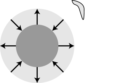
Figure 1: Geometry of our model stellar system. The hypothetical central star is a radially pulsating O or B star (see text.) As the star expands and contracts, the surface temperature changes the emitted blackbody spectrum, and thus varies the availability of UV photons of different wavelengths. Hot, X-ray emitting gas with temperature in the range of $10^{6}$ K and containing He-like ions is located on-order 1 $r_{\star}$ above the surface.

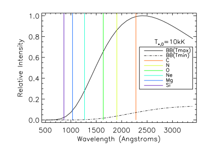
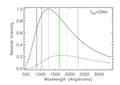
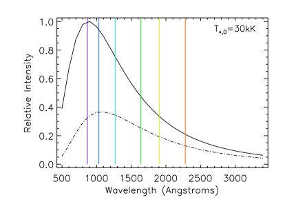
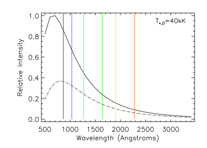
Figure 2: Blackbody spectra at maximum (solid line) and minimum (dot-dashed line) temperature over the course of the pulsation for our hypothetical stars with average effective temperature of 10,000, 20,000, 30,000 and 40,000 K (top to bottom). UV-pumping wavelengths for 6 helium-like ions are also shown for reference, C v (red), N vi (yellow), O vii (green), Ne ix (teal), Mg xi (blue) and Si xiii (purple).

3 Results

We have calculated the time-variability of $R$ for six helium-like ions around three hypothetical radially-pulsating B stars and one low-massloss O star. The main parameters of these systems are listed in Table 2. For our main discussion, we will present simulations for X-ray emitting gas located at $r_{\rm gas}=2r_{\star}$ as a fiducial value. This model, with the gas at a discrete location, may be applicable in some stellar systems, especially if the X-ray emitting gas were constrained by magnetic fields. The exact location of the gas has implications for our results. We therefore have performed simulations with the gas at different distances. In general, placing the gas closer to the surface of the star increases the intensity of the radiation field uniformly, and therefore increases the pumping in each ion and reduces the ratio $R$; increasing the distance has the reverse effect. In addition, because the radiation field has less impact on $R$ in general when the gas is located further away, any change in the radiation field will also have a smaller effect on $R$ in an absolute sense.

In the more general case, the hot gas may be distributed in radius around the star. Unfortunately, the exact distribution of gas is highly model dependent, and the results will be strongly dominated by the location of the inner radius. (See Leutenegger et al. (2006) for a more in-depth discussion of this issue.) We therefore calculated the effect of all possible distributions on our model. Fig. 3 plots $R/R_{0}$ versus location of the gas. Here we use inverse distance from the star, $u=r_{\star}/r$, with the inner radius of the X-ray emitting gas located at $u=u_{0}$. The solid line shows the impact on $R$ if the gas is distributed from $r_{0}$ to infinity ($u_{0}$ to 0), whereas the dotted line shows $R$ if the location of gas is confined only to $u_{0}$. Note that the value of the dotted line at $u_{0}=1/2$ is equivalent to $r_{\rm gas}=2r_{\star}$.

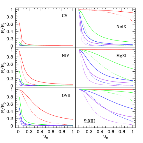
Figure 3: Effects of the spatial distribution of X-ray emitting gas on the behavior of $R$ for six helium-like ions: C v (top left), N vi (middle left), O vii (bottom left), Ne ix (top right), Mg xi (middle right) and Si xiii (bottom right) for each of our hypothetical stars with average effective temperature of 10,000, 20,000, 30,000 and 40,000 K (red, green, blue, and purple respectively). $R/R_{0}$ is plotted versus inner radius of gas in inverse radius $u_{0}$. The substitution of variables, $u=r_{\star}/r$, simplifies the calculation. The solid line indicates how much $R$ is depressed from its nominal value if the gas is distributed from $r=\infty$ ($u=0$) to $r=r_{0}$ ($u=u_{0}$). The dotted line shows the results if hot gas exists only at $u_{0}$. The value or the dotted line at $u_{0}=1/2$ is equivalent to our fiducial value elsewhere of $r_{\rm gas}=2r_{\star}$ at zero displacement phase.

This figure shows that there can indeed be a significant difference in the $R$ ratio due to location and distribution of the gas. Of course, the difference is generally larger the closer the inner radius of the gas is to the surface of the star. The smaller radius increases both the impact of a varying UV field on the closer material, and the total amount of emitting material. In most cases, however, the difference between gas confined at a single location and gas extending to infinity is at most on order of the difference between two stellar temperatures, i.e. between $T_{\star,0}=20,000$K and $T_{\star,0}=30,000$K.

Given the uncertainties inherent in modeling a spatial distribution, from here on we return to the fiducial location of $r_{\rm gas}=2r_{\star}$. Our simulations investigate the effects of three factors: temperature of the star, a phase offset between the radial and temperature variations, and the cyclical variation in location of the gas above the surface of the star. We refer to these as the temperature effect, phase effect, and W effect, respectively. Fig. 4 shows the variation of $R$ over time for each combination of the these factors, for the six helium-like ions as labeled. Every ion does respond to some degree at each stellar temperature. But the size of the response in each ion is quite different. At a given temperature, the radiation field will either almost completely suppress $R$ (in ions with lower energy UV-pumping photons; note the scale of variation in Fig. 4), or have little impact at all (in ions with greater separation between the triplet energy levels.) In the former case, $R$ itself will be hard to measure observationally; in the latter, any variations will be small and likewise difficult to detect.

At each temperature there are one or two ions where the pumping frequency is in the right portion of the stellar spectrum to substantially affect the level populations but not totally depopulate them. In these ions, changes in the radiation field may have a significant, potentially observable effect on $R$. Table 3 shows the statistics of variation for each ion for each of our stellar temperature models in the fixed-gas, no-phase-offset simulations. The first column shows $R_{0}$ from Blumenthal et al. (1972), the fiducial value that all changes are relative to. $\left<R\right>$ is the time-average value of $R$ found in each simulation. $\sigma_{R}$ is the standard deviation of the variation in $R$ with phase. If the shape of the $R$ curve was sinusoidal, in the form $R=a+b\sin(\xi)$, then $a=\left<R\right>$ and $b=\sigma_{R}$. But as Fig. 5 shows, $R$ is not always sinusoidal, and in those cases these values have a different relationship to the overall behavior with time. The fifth column of Table 3 shows how much the value of $R$ has been depressed from the nominal value (the case of no radiative pumping), while the sixth column shows the scale of variation relative to the average value. These two columns provide a sense of the observability of the ratio and the potential to detect the variations in the ratio, respectively.

These results are presented in another way in Fig. 4. These plots also demonstrate the impact of a phase offset between the temperature and radius variations in the star, and of oscillating versus fixed gas. If $\psi=0$, the maximum in $R$ always occurs at the same phase as the minimum in star temperature, whether the gas is moving in time with the surface of the star or not. This is because the number of available UV photons is mostly set by the temperature of the star, and if the gas is moving with the star, the change in radius has no effect on the radiation field at the gas location. If, however, the gas is fixed and the star moves outward at the same time the temperature increases, both factors work to increase the intensity of the radiation field.

In the non-synchronous variability case ($\psi\neq 0$), if the emitting gas is moving with the radius of the star, the line ratios will have similar properties to the synchronous case, but with an offset in phase. This is because changes in $R$ are almost completely due to changes in the temperature of the star. If the gas is fixed, on the other hand, the effect is the reverse of the $\psi=0$ case – diminishing the change in $R$ rather than increasing it, because the increase in intensity from being closer to the surface of the star works to counteract the increase in intensity due to a higher stellar temperature. The changes in the temperature still dominate, however. If $\psi=0.5$, the maximum $R$ will still occur at the same time as the minimum $T_{\star}$; at any other $\psi\neq 0$ offset, the maximum $R$ will occur just after the minimum stellar temperature, as the stellar surface begins to approach the gas.

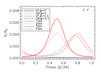
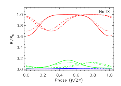
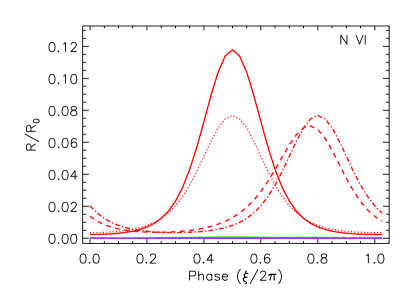
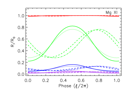
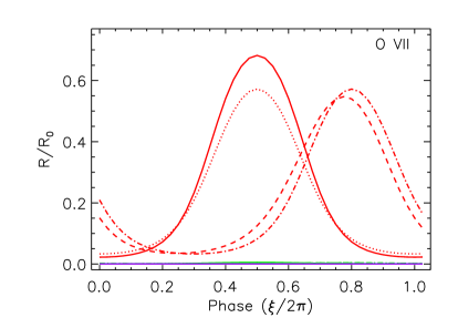
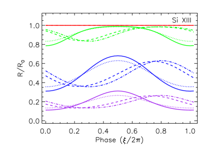
Figure 4: Effects of temperature, phase offset, and gas motion on the behavior of $R$ for $r_{\rm gas}=2r_{\star}$ for six helium-like ions. The ions are C v (top left), N vi (middle left), O vii (bottom left), Ne ix (top right), Mg xi (middle right) and Si xiii (bottom right). Simulation temperatures are 10,000, 20,000, 30,000 and 40,000 K (red, green, blue, and purple respectively). “GF” refers to simulations where the gas remains at a fixed distance from the center of the star, while “GM” signifies simulations where the gas moves in time and proportion to the radial motion of the star. Thus the solid line is at fixed distance with no pulsation radial-temperature phase offset; the dotted line is moving gas with no offset; the dashed line is fixed gas with an offset; and the dot-dashed line is moving gas with a phase offset. Note that the scale of the plots for the lighter elements is reduced to show the range of variation, which can be quite small.

Table 3: Model results for for the three stars listed in Table 2 with no temperature-radius phase offset and fixed gas location.

Ion	$R_{0}$ 1	$\left<R\right>$	$\sigma_{R}$	$\left<R\right>/R_{0}$	$\left<R\right>/\sigma_{R}$
$T_{\star,0}=10,000$K
C v	11.30	0.02	00.02	$<$0.01	0.89
N vi	05.13	0.16	00.20	00.03	0.83
O vii	03.85	0.91	00.92	00.24	0.98
Ne ix	03.17	2.71	00.48	00.85	5.65
Mg xi	03.03	3.02	00.02	01.00	$>$100
Si xiii	02.51	2.51	$<$0.01	01.00	$>$100
$T_{\star,0}=20,000$K
C v	11.30	$<$0.01	$<$0.01	$<$0.01	01.68
N vi	05.13	$<$0.01	$<$0.01	$<$0.01	01.53
O vii	03.85	$<$0.01	$<$0.01	$<$0.01	01.41
Ne ix	03.17	00.21	00.17	00.07	01.30
Mg xi	03.03	01.49	00.68	00.49	02.18
Si xiii	02.51	02.27	00.19	00.91	11.80
$T_{\star,0}=30,000$K
C v	11.30	$<$0.01	$<$0.01	$<$0.01	3.00
N vi	05.13	$<$0.01	$<$0.01	$<$0.01	2.79
O vii	03.85	$<$0.01	$<$0.01	$<$0.01	2.60
Ne ix	03.17	00.03	00.01	$<$0.01	2.29
Mg xi	03.03	00.28	00.13	00.09	2.22
Si xiii	02.51	01.20	00.34	00.48	3.51
$T_{\star,0}=40,000$K
C v	11.30	$<$0.01	$<$0.01	$<$0.01	3.29
N vi	05.13	$<$0.01	$<$0.01	$<$0.01	3.11
O vii	03.85	$<$0.01	$<$0.01	$<$0.01	2.95
Ne ix	03.17	$<$0.01	$<$0.01	$<$0.01	2.65
Mg xi	03.03	00.09	00.04	00.03	2.45
Si xiii	02.51	00.49	00.18	00.19	2.68

(1) Blumenthal et al. (1972).

Table 4: Some values of scales of $R/\delta R$ in a sample of stars with observed $R$ ratios from the literature. This measure shows the potential observability of variability of the ratio in different lines for these stars, not a variation that has been detected.

Object	S xv	Si xiii	Mg xi	Ne ix	O vii	N vi	C v	Reference
$\zeta$ Pup		4.50	4.00	2.92				1
$\zeta$ Ori		1.19	2.25	1.50				1
$\xi$ Per		0.154	1.27	1.00				1
$\zeta$ Oph		1.125	3.00	1.00				1
$\tau$ Sco		3.00	3.46		5.60	3.09	1.48	2
$\tau$ Sco	1.88	7.78	6.86	$R<$0.03	$R<$0.13			3

(1) Oskinova et al. (2006); (2) Mewe, R. et al. (2003a); (3) Cohen et al. (2003).

Fig. 5 shows the difference in response of $R$ to stellar pulsations for the different ions in the fixed-gas, no-phase-offset case. Note that the absolute scale of variation changes dramatically between ions – see Table 3 for values of $\left<R\right>$ and $\sigma_{R}$. In heavy ions at lower temperatures, there are few photons at the wavelengths needed to depopulate the forbidden line level, and consequently $R\sim R_{0}$. As the temperature increases, more depopulating photons become available, and $R$ varies with phase. Eventually even the heaviest ions have enough photons to saturate the response, and the profiles of all ions show the same shape, though the absolute scales still differ. This divergence from sinusoidal response at moderate intensity impacts the root mean square of the value of $R$ of each ion, and thus the expected value for $R$ if observed in this regime. Fig. 6 demonstrates these trends and shows the behavior of $R$ for each of our six ions in relation to the approximate visible light curve of the pulsating star. The approximate visible magnitude here is calculated by finding the total flux from the blackbody spectrum in a 64 nm band centered on 540 nm.

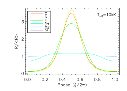
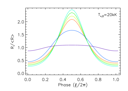
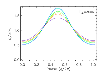
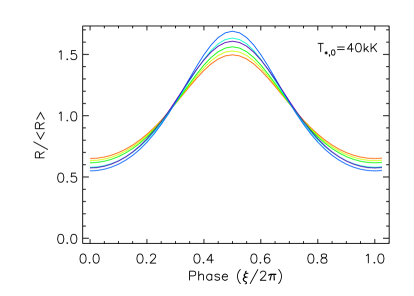
Figure 5: Variation in ratio $R/\left<R\right>$ for each of the six helium-like ions, C v (red); N vi (yellow); O vii (green); Ne ix (teal); Mg xi (blue); and Si xiii (purple), for our model for a star with average effective temperatures 10,000, 20,000, 30,000 and 40,000 K (top to bottom). Note that the absolute scale of variation changes dramatically – see the values of $R_{0}$ and $\left<R\right>$ for each ion in Table 3. This figure shows the differences in the width and height of the peaks and troughs in the periodic variation of the ratio.

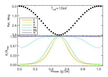
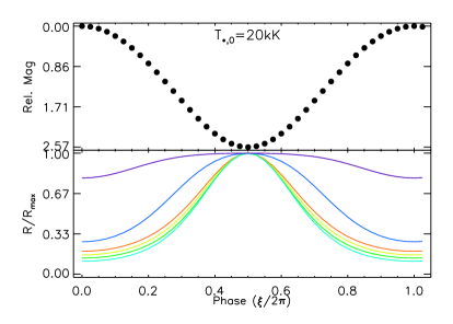
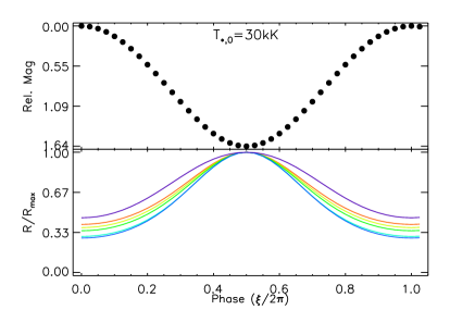
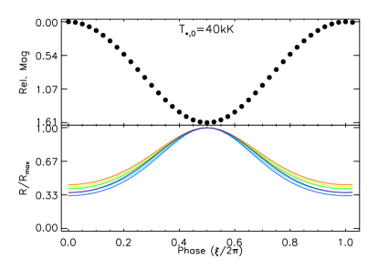
Figure 6: Variation in $R$ versus approximate visible magnitude light curve (dots; see text) for six helium-like ions: C v (red), N vi (yellow), O vii (green), Ne ix (teal), Mg xi (blue), and Si xiii (purple); for stars with average effective temperatures 10,000, 20,000, 30,000 and 40,000 K (top to bottom). Note that the peak in $R$ corresponds with the minimum optical brightness.

Table 4 gives a sense of the current state of observational possibilities for the $R$ ratio in actual hot stars. A comparison between Table 4 and Table 3 gives a sense of how observable the variations in our simulations may be with current instruments. In the observational table, $R/\delta R$ represents the data quality typical of current observations. It is the value of the measured ratio $R$ divided by the uncertainty in that measurement; thus a value of 1 indicates uncertainty equivalent to the measurement, while a larger number means greater certainty and a greater chance of detecting variability. The value is listed for different triplet lines for different stars, as indicated. The star $\tau$ Sco appears twice: once for XMM-Newton spectra (first) and once for Chandra data (second). Note that most of the sources listed in Table 4 are early-type O stars, whereas our models are for B and late-type O stars. However, the data quality are shown primarily as a guide for the scope of what amplitude levels may be reasonably detected as compared to predicted amplitudes of variations.

$\left<R\right>/\sigma_{R}$ is the equivalent value from our simulations (Table 3), yet here the implication for observability is different. If $\left<R\right>$ is small, the total flux will be low and therefore hard to measure, requiring a small signal-to-noise ratio and long exposure times. Further, if $\sigma_{R}$ is small, the change in $R$ at any time will be small, and harder to detect. Thus to be detectable, we need an $\left<R\right>\gtrsim 0.1$ and $\sigma_{R}\sim\left<R\right>$.

To summarize the detection possibilities, the only ions in our simulations that seem to be candidates for such detection are Ne ix for the $T_{\star}=10,000$K star and Mg xi and Si xiii for the $T_{\star}=20,000$ and 30,000K stars. It might be possible, though hard, to detect variation in Si xiii around a $T_{\star}=40,000$K star. Though our simulations are coarsely gridded, these results are likely to be robust, since the only element between Ne ix and Mg xi is Na x, which is not commonly seen in observations. Bear in mind that these simulations were designed for maximum variability and detectability. A variety of factors, discussed in the next section, could make actual detection more difficult.

4 Discussion

We have investigated variability in $R$ for He-like ions in massive stars, caused by cyclical changes in the radiation field of a star. We have made several simplifications that allow us to explore the upper limits of the possible effect of stellar pulsation on observed variability in $R$: we have assumed a hot O or B star with purely radial pulsation to maximize the influence of radiative pumping effects on X-ray diagnostic $R=f/i$. We have chosen a B or low-mass loss O star, so that we could plausibly assume that the electron density in the gas is much lower than the critical density, so that $R$ is determined solely by the stellar radiation field. And we have assumed an X-ray emitting gas with a range of temperatures $\sim 10^{6}-10^{7}$ K, to isolate the effect of the radiation field from more complicated effects of changes in $R_{0}$, $T_{X}$, and ionization fraction within the gas. We have also confined the emitting gas to a single location, which isolates the response to the local UV radiation field rather than integrating over many locations and UV flux densities. This model might be applicable for an early B or late O star with a strong magnetosphere to magnetically channel or confine the hot gas near the stellar surface.

With these optimizing assumptions, our model predicts that a variation in the $R$ ratio could be detectable in one or two lines simultaneously. This is because, with a reasonable blackbody spectrum variations changing UV flux, the value of $\phi_{c}$ and the pumping wavelength have sufficient dynamic range that most lines are in one or the other limiting case: virtually no pumping or extreme pumping. Our model predicts which lines should be variable for stars of different surface temperatures. Thus observations of this kind could be used to probe the environment of pulsators or stars with magnetically confined wind shocks. $\beta$ Cephei, a B-type star at a distance of 182 pc, could be an interesting target for such analysis. The prototype for $\beta$ Cepheid class variables, it has known variability, with a main pulsation mode period of 274 minutes and other non-radial modes (Favata et al. 2009).

If variability were observed in $R$ in several lines at once, however, our model makes it unlikely that variations in the radiation field alone could be responsible. Even with many optimizing assumptions, we find that the effect on $R$ is not likely to be observable in more than two lines simultaneously. Our simulations show that either the line will already be depopulated – and $\left<R\right>$ so depressed as to be itself undetectable, let alone variations in $R$ – or the line will be mostly unaffected, and any variation due to stellar pulsations will be too small to be observable.

We do note that even where our simulations found potentially observable variation, it would likely be more challenging to measure in practice than in our model. As mentioned above, our phenomenological model has been tailored to produce the maximum detectable effect, and any attempt to include more ingredients will reduce even the effects seen here. In hotter O stars, line formation is more complex, with the possibility of photo-absorption of X-rays in the wind, diluting the impact of changes in the radiation field such as those modeled here. In a non-radial pulsator, temperature and radius do not vary smoothly across the stellar surface, minimizing the spectral variations and the changes in dilution at the location of the gas. Further, adopting a multiple-temperature gas with varying ionization fractions for each element may decrease the response of the level populations in the gas and thus of $R$ in each ion.

Finally, a stellar spectrum is not actually a blackbody. In any region of the spectrum that is generating UV photons in the appropriate range, there will be photospheric absorption lines. If an absorption line corresponds precisely to the pumping frequency, $R$ will not be affected, either by the UV flux or by its variation. If the X-ray emitting gas is spatially distributed within the wind, it is likely that an absorption line will fall somewhere within its range of Doppler-shifted velocities. Further, the Lyman edge means that there will be fewer photons available below 912${\rm\AA}$ than are present in our model. In any atom with He-like ion pumping wavelength below the Lyman edge, e.g., silicon and all heavier elements, the true impact on $R$ will be less than that in our model and $R$ will be closer to $R_{0}$.

For these reasons, it seems likely that changes in the radiation field will not be able to fully account for the reported time variations in $R$ in hot stars across several lines. Instead, future studies must explore the impact of changes in density surrounding the star, through mass-loss changes, clumping in the stellar winds, ejection events and magnetic field effects. Such models will provide us with new tools for understanding the environment of these hot stars, and their interactions with it.