Current address: ]Massachusetts Institute of technology 77 MA, Bldg 13-3061, Cambridge, MA 02139.
Quantum resonant effects in the delta-kicked rotor revisited
Abstract
We review the theoretical model and experimental realization of the atom optics kicked rotor (AOKR), a paradigm of classical and quantum chaos. We have performed a number of experiments with an all-optical Bose-Einstein condensate (BEC) in a periodic standing wave potential in an AOKR system. We discuss results of the investigation of the phenomena of quantum resonances in the AOKR. An interesting feature of the momentum distribution of the atoms obtained as a result of short pulses of light, is the variance of the momentum distribution or the kinetic energy in units of the recoil energy . The energy of the system is examined as a function of pulse period for a range of kicks that allow the observation of quantum resonances. In particular we study the behavior of these resonances for a large number of kicks. Higher order quantum resonant effects corresponding to the fractional Talbot time of (1/4) and (1/5) for five and ten kicks have been observed. Moreover, we describe the effect of the initial momentum of the atoms on quantum resonances in the AOKR.
pacs:
05.45.Mt,32.80.LgI Introduction
In classical dynamics, small perturbations in the initial conditions of a system may grow exponentially with time and produce large ones in the final states. This makes the motion practically unpredictable, and the phenomenon is known as classical chaos Lichetenberg and Lieberman (1992); Lieberman and Lichtenberg (1972); Kornfeld et al. (1982); Chirikov (1979). On the other hand, the investigation of the behavior of quantum systems, the classical limit of which are chaotic, has brought up a new discipline in physics, which is now known as “quantum chaos”. The pioneering work by Giulio Casati and co-workers predicted that a quantum particle shows diffusion following the classical evolution, after a certain time known as the quantum break time Casati et al. (1979); Chirikov et al. (1981); Shepelyanski (1983). The diffusion stops due to quantum interference, beyond the quantum break time, leading to dynamical localization Moore et al. (1995); Ammann et al. (1998) which is analogous to Anderson localization in solid state physics.
The strange connection between classical chaos and quantum chaos has forced people to develop models that can describe systems that are chaotic. The kicked rotor is one of the simplest models that is useful to understand classical and quantum chaos. The classical model of the kicked rotor is a simple pendulum that is kicked periodically by an external force. The dynamics of the the pendulum that exhibits chaos can be described by the Hamiltonian mechanics. Classically a kicked rotor is a well known system that makes its quantum analogue the best model to study quantum chaos Moore et al. (1995); Ammann et al. (1998); Stöckmann (1999); Fishman (1993).
The quantum analogue of the classical kicked rotor is obtained by a cloud of ultra cold atoms interacting with a pulsed standing wave of laser light and is known as atom-optics kicked rotor (AOKR). The atom-optics realization of the kicked rotor was first demonstrated by the Raizen group Moore et al. (1995) in 1995, and has been studied extensively theoretically and experimentally in Casati et al. (1979); Izrailev and Shepelyansky (1980); Izrailev (1980); Saunders et al. (2007); Halkyard et al. (2008); Saunders et al. (2009); McDowall et al. (2009); Saif (2005) and Wimberger et al. (2003); Wimberger and Sadgrove (2005); Deng et al. (1999); Oberthaler et al. (1999); Szriftgiser et al. (2002); Duffy et al. (2004); Jones et al. (2007); Wayper et al. (2007); Currivan et al. (2009); Ullah and Hoogerland (2011) and the references therein. The AOKR model has allowed experimental studies of the phenomena of “quantum resonances” Fishman et al. (1982); Wimberger et al. (2003) that occur due to the matter-wave Talbot effect Ryu et al. (2006); Deng et al. (1999); Ovchinnikov et al. (1999); Lepers et al. (2008), analogous to the optical Talbot effect Talbot (1836).
An interesting feature of the momentum distribution of the atoms obtained as a result of short pulses of light, is the variance of the momentum distribution or the kinetic energy , in units of recoil energy , where , where is the wavelength of the laser beam and the mass of the atom. The energy of the system is examined as a function of pulse period.
In this paper, we present some of the known results along with our new results to illustrate the phenomena of quantum resonances in the AOKR. We also present experimental observation of higher order quantum resonances corresponding to the fractional Talbot time for five and ten kicks. The results are in good agreement with those presented in Ryu et. al. Ryu et al. (2006), where higher order resonances were found in a similar experiment with a condensate of Na atoms. Moreover, in section III, the dependence of the initial momentum of the atoms on quantum resonances have been discussed in detail. The results presented are in good agreement with those proposed in Saunders et al. (2007).
II Theory
The general Hamiltonian that describes the dynamics of atoms in the Atom-Optics kicked rotor experiment can be expressed as
| (1) |
where is the kick period and is the kick strength. The kick strength , which is determined by the effective Rabi frequency during the laser pulse and the pulse length . The effective Rabi frequency is defined as .
II.1 Evolution of the wave packet
The time evolution operator that determines the evolution of the wave function from one kick to immediately after the next kick is known as the Floquet operator Currivan et al. (2009); Saunders (2009); Sadgrove (2005). In general, the state of the system after number of kicks can be found by the Floquet operator acting on the initial state i.e.,
| (2) |
In the first part of the Hamiltonian describing the quantum kicked rotor, the system evolves freely via the operator
| (3) |
Then delta kicks act for a small period of time, and the evolution is given by the operator
| (4) |
Combining the above two operators, the Floquet operator is given by
| (5) |
or in a more general form as
| (6) |
From the definition above, the action of each kick on the atoms, which is governed by is followed by a phase of free evolution . A more detailed description of the evolution of the quantum wave packet for a delta kicked rotor system can be found in Saunders et al. (2007).
II.2 Simulating the AOKR
In order to simulate the AOKR, the well-known split operator method for the time evolution of the Floquet operator has been used, which is ideally suitable for the experiment with grid points, as described in detail in Currivan et al. (2009) and Ullah and Hoogerland (2011). As described in the previous section, the time evolution of the quantum kicked rotor can be separated into two parts: The evolution of the system during the time when laser pulses are applied on the atoms as kicks, and the evolution during the time of free expansion in between the kicks. The kick potential is a diagonal operator in position space, whereas the free evolution is a diagonal operator in momentum space. Therefore, for the time evolution of the system, a Fourier transformation is used in order to transform the wave function from position space into momentum space and back again. The initial wave function representing the state of the system can be defined as
| (7) |
The width of the initial wave packet is chosen such that it covers several wavelengths of the kick laser.
For the kicking part of the time evolution, the delta-function is represented by a block function with a width and an area Currivan et al. (2009). The initial wave function in position space in the simulation is multiplied by
| (8) |
The wave function is then transformed from position space into momentum space represented by using an inverse Fourier transform. The free evolution part of the system can be determined by multiplying the wave function in momentum space by
| (9) |
which gives the final state in the momentum space . The parameter represents the pulse period in between the kicks. After the free evolution part, the wave function is transformed back to position space by applying the Fourier transform and gives the updated state . The process is repeated for each kick, giving us the updated wave function each time after the evolution. The momentum and energy of the atoms after each kick is then determined.
II.3 Quantum resonances in AOKR
Quantum resonances are well known quantum effects that occur for specific initial conditions and certain values of the kicking period. We investigate these resonances in the AOKR by considering the atoms diffracted by a standing wave potential. A “quantum resonance” exists for , being the Talbot time, where all kicks add coherently and energy grows quadratically with the number of kicks. An “anti-resonance” is observed at , where the effect of each kick is effectively negated by the following kick.
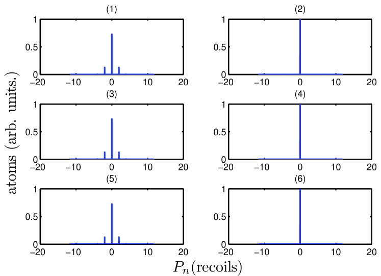
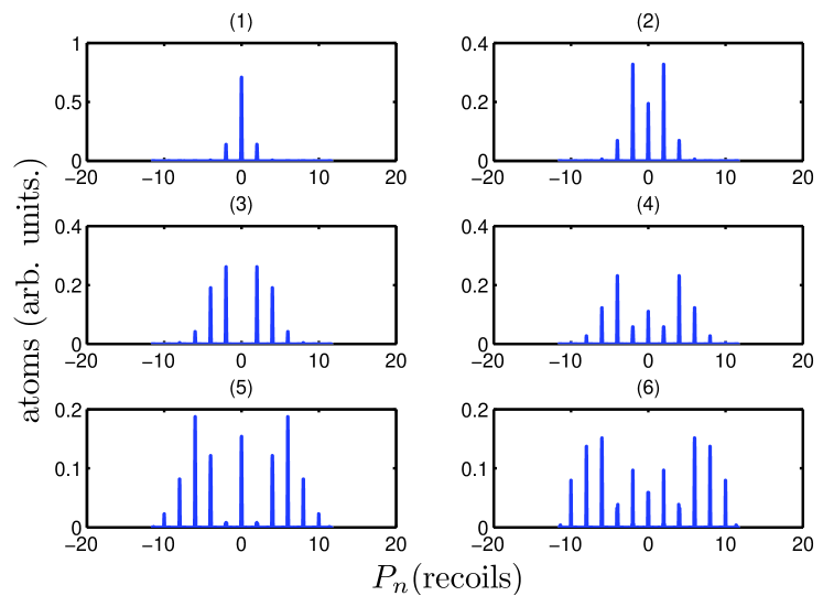
The free evolution term is of primary importance in describing the quantum kicked rotor. If the initial state is assumed to be a momentum eigenstate , and let the operator act on it such that , then the evolution is different for different values of . If is an even multiple of , then the free evolution results in unity. This means that the free time evolution in this case does not have any effect on the state vector of the system. The system responds only to the kicks Saunders (2009), and the evolution is fully governed during interaction with the kicking potential. This is the condition for quantum resonance Izrailev and Shepelyansky (1980). On the other hand, if is an odd multiple of , then the initial momentum eigenstate acquires different quantum phases for even and odd . The state after the free evolution acquires a quantum phase of for even values of , whereas for odd the quantum phase results in . For odd values of the momentum components of the wave-function, the phase of leads to an oscillation of the energy of the system. Therefore, is known as the quantum anti-resonance condition for the kicked rotor Oskay et al. (2000); Sadgrove et al. (2005). The phenomenon of quantum resonance and quantum anti-resonance is demonstrated in the simulations in Figures 1 and 2 respectively.
The general expression for the order momentum moment of the kicked particle after time as expressed in Saunders et al. (2007) is given by
| (10) |
The parameter is defined as
| (11) |
where is the quasimomentum. Quantum resonant and antiresonant behavior of the system can be characterized by the second order momentum moment for , and is proportional to the kinetic energy.
As discussed in the previous sections, the evolution of the system can be determined by the time evolution operator. In the case of quantum resonance, the free evolution part is unity, therefore for kicks the evolution operator is written as
| (12) |
where is the kick strength. The final state of the system is as if a single kick had been applied with a strength times the original kick strength . The probability for an initial momentum state , to be populated in the final state after kicks is given by
| (13) | ||||
| (14) |
Using the definition of orthogonality of the momentum eigenstate and the identity , where is the ordinary Bessel function of order , we get
| (15) |
For a system that starts in a zero momentum eigenstate, the final momentum distribution becomes
| (16) |
The energy of the ensemble after kicks can also be found at the quantum resonance, and is given by
| (17) |
For a kicked rotor starting in the zero momentum state, the above result shows a quadratic growth in energy for kicks for the quantum resonance.
II.4 Experimental effects
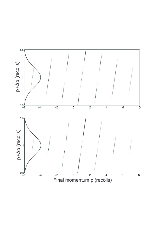
In the experiment, the initial momentum distribution from the BEC has a width of recoils. The initial width associated with the BEC qualitatively alters the momentum distribution after the kick sequence. In an ideal case the initial momentum distribution is a delta function at , however in reality, the initial momentum distribution has a width. Because of this width, there are some atoms at a momentum , where the quantity is much smaller than one recoil. In order to take into account this initial momentum width, we performed the simulation for a range of initial momenta. In Fig. 11, the probability of finding the atom at a final momentum is plotted for a range of initial momenta for both antiresonance (top) and resonance (bottom). The initial momentum distribution of the BEC is also displayed (as a solid curve). The effect of the initial momentum on the system can be observed as a transfer of the probability of atoms to states at small offset momenta. As the probability is very sensitive to the initial momentum, this sensitivity therefore translates into peaks appearing at a small offset momentum which are not present at , where is equal to one recoil in this case. Conversely, this can also be seen as a peak disappearing at which was present at . The resulting momentum distributions are then added incoherently, weighed by the height of the momentum distribution of the original BEC at . The final momentum distribution is obtained by the sum of horizontal profiles in Fig. 11 weighed by the initial momentum distribution.
III Experimental observation of quantum resonances
III.1 Experimental Setup
We use a double magneto-optical trap (MOT) configuration for the formation of all-optical Bose-Einstein Condensate (BEC) of () 87Rb at a temperature of 50 nK. The all-optical BEC of atoms is formed in a cross dipole trap created by a pair of intersecting focused CO2 laser beams. A detailed description of the experimental setup can be found in Wenas and Hoogerland (2008).
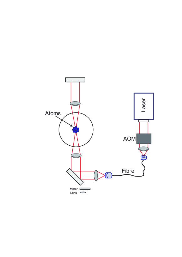
We realise the AOKR by pulsing a near resonant optical standing wave, derived from a 780 nm diode laser, onto a BEC of 87Rb atoms. The kick laser is locked to the transition in the 85Rb isotope. Hence, the laser frequency is detuned by 2.45 GHz from the relevant resonance frequency. The laser beam from the diode laser passes through an acousto-optic modulator (AOM) for fast switching. After passing through the AOM, the beam passes through a single mode optical fibre and is focused onto the BEC. The beam diameter at the focus is 100 m, much larger than the size of the BEC (10 m), thereby yielding a constant interaction strength over the BEC, while increasing the intensity. After passing through the center of the trap the linearly polarized beam is then retro-reflected to produce a standing wave. The kick laser setup is shown in Fig. 3.
In the AOKR experiment, the BEC is illuminated with short pulses of light in the form of a standing wave. The standing wave potential or the interaction potential acts like a diffraction grating, which changes the atomic momentum, and the BEC eventually splits into a number of momentum components. An alternate picture is that the atoms absorb a photon of momentum from one beam, and then provide another photon through stimulated emission in the other beam. The diffracted components of momentum are therefore separated by . In order to reduce mean field effects, the trap that contains the BEC is turned off s before the kick sequence is applied. A shutter is used in the laser beam to ensure that it is totally extinguished during the evaporation phase to create the BEC.
The periodic potential is related directly to the intensity of the laser beam and inversely to its detuning from the atomic resonance. High laser power allows the experiment to be done at large detunings to suppress spontaneous emission. Therefore, for the interaction potential it is desirable to get as much power as possible from the kick laser. The total laser power of the experiment can be varied up to 2 mW. The laser pulses are so short that the evolution of the wave packet due to its momentum can be ignored during the kicking time. Atoms satisfying this condition are said to be in the Raman-Nath regime Currivan et al. (2009); Sadgrove (2005).
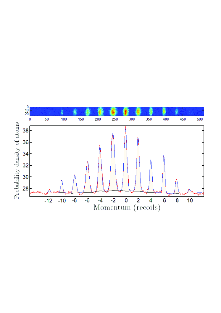
The momentum distribution of the atoms after the kick sequence is measured by absorption imaging using the time-of-flight technique, with a typical flight time of 5 to 10 ms. Just prior to imaging, the atoms are optically pumped to the state by a 100 s pulse on the repump transition. An absorption image is then obtained using a probe laser which is tuned to the transition. The two dimensional momentum distributions obtained are summed over the width of the cloud to obtain a one dimensional momentum distribution. The energy of the atoms is then obtained by the variance of the momentum distribution by fitting a number of Gaussians, one to each diffraction order. A typical example of the fitted momentum distributions is shown in Fig. 4.
III.2 Results of the primary quantum resonances
The kinetic energy of the system in the case of a standing wave potential as a function of pulse period is studied for a range of pulses or kicks. This situation can also be thought of as equivalent to that of varying the spatial distance between the gratings in the optical Talbot effect. To start with, the energy is measured by scanning the pulse period (time delay) for two kicks. The period between the kicks is varied from () s. The second kick is used as a tool to study the time evolution of the wave function after the first kick. It is well known that in the atomic version of the kicked rotor, at the Talbot time s of free evolution, an identical wave function to that directly after the first kick is observed. The introduction of another grating or kick at the Talbot time then simply doubles the effect or duration of the first kick. As a result, a quadratic growth in energy is observed Reichl (1992); Izrailev and Shepelyansky (1980).
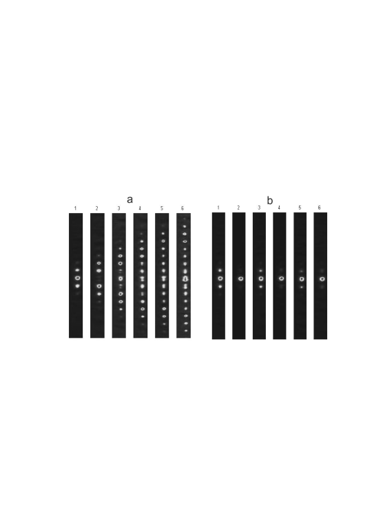
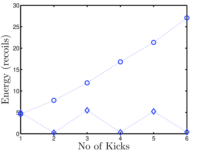
At a pulse period of s, which is equivalent to half of the Talbot time, i.e. , the quantum phase factor between kicks alternates sign Oskay et al. (2000). As a result, a re-image of the grating’s transmission function, which is the inverse of the initial one, is obtained. In effect, two kicks with half the Talbot time in between them results in the complete negation of the effect of the first kick. The quantum resonance and anti-resonance behavior is observed in the experiment as shown in absorption images in Fig. 5 a and b (Top) with the corresponding energy of the atoms representing these resonances (Bottom).
III.3 Intermediate secondary resonances
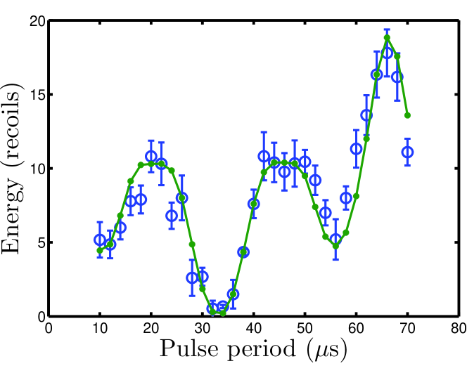
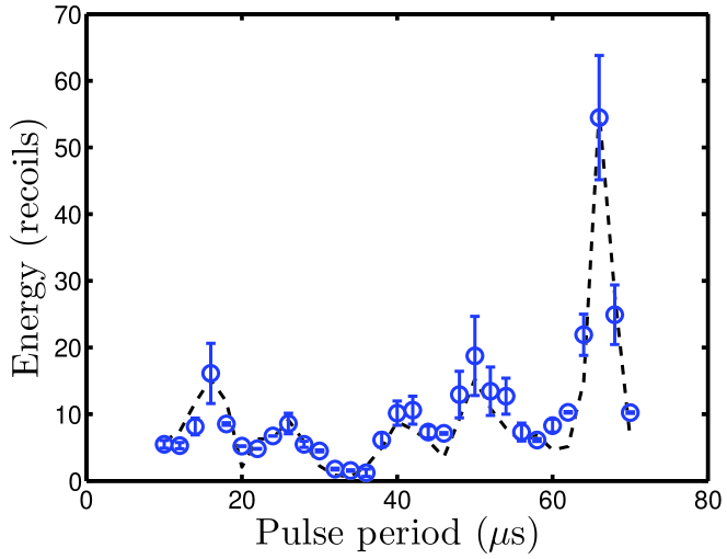
The energy dependence of the condensate diffracted by two gratings or kicks as a function of pulse period between the kicks is shown in Fig. 6. The solid curve represents the theoretical simulations, whereas the circles are the experimental observations. The error bars are determined by running the experiment a number of times. The well defined peaks and valleys that are observed correspond to the integer and fractional Talbot times. The maximum in energy at s is in close resemblance with the simulation, and is a clear indication of the Talbot time that corresponds to the quantum resonance. The minimum in energy at s is also clearly visible, matching the theoretical predictions of half the Talbot time .
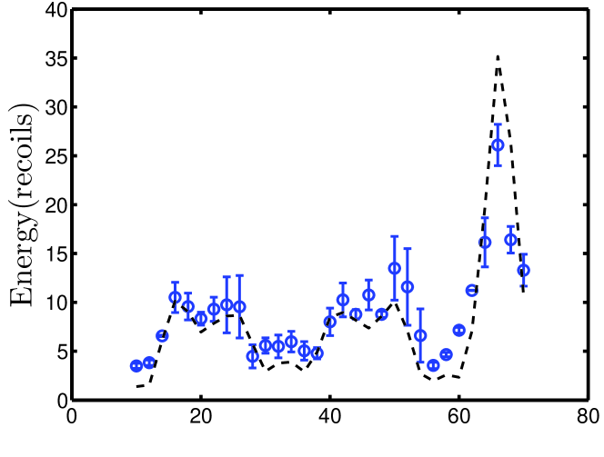
The energy of the system is also studied as a function of pulse period, by adding another pulse (kick) to the first two. The addition of this pulse increases the energy of the system by inducing an extra phase shift. The global minimum in this case is then replaced by a local maximum as the complete cancelation of the first two kicks is destroyed by the third one. This is true for an odd number of kicks. The final energy of the system for three kicks as a function of pulse period is shown in Fig. 7 (Top). Most of the structure in Fig. 7 is less visible; however, the maximum in energy at about is still obvious as the gratings for this amount of free evolution do not induce any additional phase shift.
The evolution of the system in the presence of large number of kicks shows interesting results in the simulations. By measuring the energy, the evolution is examined in the presence of four and five kicks. It is well known that with an increase in the number of kicks, the width of the quantum resonances when plotted against the pulse period becomes narrow Currivan et al. (2009); Ryu et al. (2006). In Fig. 7 (bottom), the energy as a function of pulse period is plotted for four kicks. In this case, at a pulse period of , the minimum in energy (close to zero) is observed again. As for an even number of kicks, the effect of the previous kick is canceled again for the corresponding time delay of , and almost no diffraction occurs. The maximum in energy at is again visible, since for this time delay the energy of the system increases with the addition of further kicks. It should be noted that the resonance peak observed at is narrow compared to the peak for a small number of kicks. This is in accordance with theoretical simulations, where a narrowing of the quantum resonance peaks for a large number of kicks is observed.
A similar behavior is observed when an extra pulse is added. In Fig. 8, the energy is examined by a complete scan of the pulse period up to the second primary resonance for five kicks. The minimum in energy at , which was obvious in the case of four gratings, however, is replaced by a local maximum as shown. This is because of the extra phase shift induced by the fifth grating, due to which the energy increases by some amount for the corresponding time delay. It is shown that much narrower resonance peaks are observed in this case around the quantum resonances of and 2 ( s). The maximum in the experiment in this case, however, is not in agreement with the simulation. We believe this discrepancy is caused by the limited signal to noise ratio. Because of the limited resolution of the experiment, the observation of the probability of the atoms at high momenta and detecting a small amount of diffraction orders at high momenta is difficult, which results in the reduction of the energy. Because of finite width of the initial momentum distribution the energy of the momentum distribution tends to be extremely sensitive to the population at high momenta Oskay et al. (2000). Overall, the experimental results are in good agreement with the theoretical predictions and simulations.
Higher order resonances are expected to occur in these systems at fractional multiples of the Talbot time , i.e., at
| (18) |
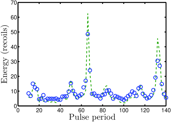
where and are integers forming a rational number. The quantum revivals, or resonances, at these fractional times are the results of superposition of copies of the initial wave packet, which are separated by Berry et al. (2001). Expecting resonances at these fractional times, the energy of the atoms is measured and plotted as a function of pulse period in between the gratings. In Fig. 9 the energy is shown for a full scan of the pulse period from s for and kicks. The maximum in energy at s is the evidence of a fractional resonance at . Similarly, the small peak at s shows another resonance which corresponds to a fractional Talbot time of .
In Fig. 9 (right), the fractional resonances become sharp as a result of large number of kicks, ten kicks in this case. For multiple gratings, the energy of the atoms is more sensitive to each induced phase shift and it is extremely difficult to analyze accurately in the experiment. The experimental data follow the general trend of those from the simulations.
IV Initial momentum dependence on quantum resonances
In this section, measurements of the effect of the initial momentum on the primary quantum resonances in the delta-kicked rotor are discussed. The study of quantum transport in such systems has been of great interest in recent years in experiments with cold atoms Sadgrove et al. (2007); Dana et al. (2008), but its dependence on the initial velocity of the atoms still needs further investigation.
IV.1 Experimental setup
In order to take into account the initial momentum dependence on the quantum resonant effects, a modified kick laser setup is used, shown in Fig. 10. The laser beam is split into two by a beam splitter, and the two beams are then passed through separate AOMs. The AOMs used for fast switching are driven in this case by an Arbitrary Function Generator (Tektronix AFG-3252), amplified by home-built RF amplifiers. The AOMs are switched on simultaneously, with a tunable frequency difference . The AFG generates two MHz (plus a desired offset frequency), Vpp sine waves that shift the frequency of the laser beams. The frequency difference gives us an effective initial momentum for the atoms, given by .

In the experiment, using the definition of , for nm one recoil frequency is given by kHz. From the definition above and in Saunders et al. (2007), kHz corresponds to a value of the quasimomentum recoils, and kHz corresponds to recoils. An equation editor ArbExpress was used to generate a pulse sequence for different pulse periods. The frequency of one beam was set at MHz and the second beam was varied by MHz+ kHz to MHz+ kHz in eight steps. By introducing the small frequency difference, a moving wave rather than a standing wave was obtained. The frequency difference corresponds to quasimomentum values of zero to two photon recoils. It should be noted that what is important is the relative phase of the sine waves driving the AOMs in the subsequent pulses, caused by the small frequency difference, not the actual frequency difference.
An ensemble of cold atoms with a momentum spread much less than a single photon recoil is used. These cold atoms are then kicked at kick periods corresponding to quantum resonances. The analytical expression for the amplitudes of the momentum states with momentum after kicks has been derived in Wimberger et al. (2003) and Saunders et al. (2007), for the kick periods that are half integer times the Talbot time ,
| (19) |
where is the quasimomentum in units of , and is an integer, given by . The parameter can be used to assign different initial momenta to the atoms in the experiment. From equation 16 and 19, the second order moment of the momentum distribution can be found as
| (20) |
The values obtained from Eqn. (19) are found to be in excellent agreement with those obtained from the simulation, and with the experimental data.
IV.2 Results and discussions
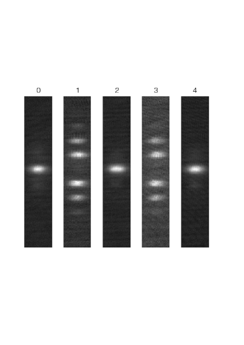
In Fig. 12, absorption images of the atoms are shown for the antiresonance case after two kicks for different initial momenta. The atoms are allowed to expand for about ms before they are imaged by the camera, using the time-of-flight method. The different initial momentum is imparted to the atoms by setting a small frequency difference between the two laser beams. At the effect of the first kick is exactly canceled by the second for the kick period corresponding to half the Talbot time, and we see almost no diffraction, as expected from the Talbot effect. At the initial momentum of , we see strong diffraction, as corresponds to a resonance for these atoms. A similar effect is observed for atoms with an initial momentum of . For atoms with an initial momentum of and there is again no diffraction. The reason for the absence of diffraction in this case is due to the fact that corresponds to an antiresonance for these atoms. For the antiresonance case here, the free evolution part of the Floquet operator evolve according to
| (21) |
and depends on the initial momentum. For the free evolution operator depends on , resulting in resonances and antiresonaces for specific values as described. The laser field induces coupling only between momentum eigenstates differing in momenta by integer multiples of Saunders et al. (2007).
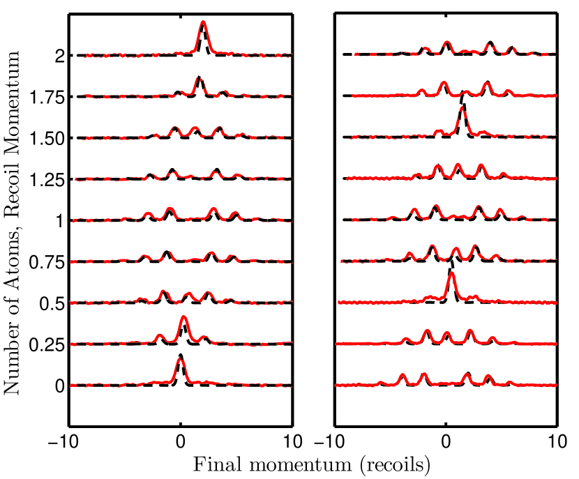
The dynamics of the system are examined for a range of initial momentum at pulse periods of and between the kicks. In Fig. 13 on the left, the momentum distribution of the atoms after the kick sequence is examined for the initial momentum in 8 steps, from 0 to 2 . The resulting 1D momentum distributions, averaged over the three repeats of the experiment, are shown as a function of the final momentum for two kicks. It can be seen that at zero velocity, there is indeed an anti-resonance and very little diffraction occurs. For small increments in the initial momentum, small peaks start to appear at higher diffraction orders. At , the first and second order diffraction peaks are observed. At an initial momentum of , the evolution turns into a resonance, with significant diffraction. The probability of atoms at higher momenta starts to decrease for and at the system returns back to an anti-resonance, with very little diffraction. Also shown in the figure are the results of the simulation. When experiments are performed with a broad initial momentum distribution, an average over many different yields an observed resonance at , as has been shown in many publications, see e.g. Oskay et al. (2000).
On the right in Fig. 13, the resulting 1D momentum distributions in the experiment and the simulations are shown for a period between the kicks of . The initial momentum is again varied from to in 8 steps. At an initial momentum of , there is a resonance and strong diffraction occurs as expected. The evolution of the system, however, turns into an antiresonance at with small diffraction, and back to a resonance at . The probability of atoms occupying the higher momentum states start to decrease again, and at an antiresonance is observed. The evolution finally turns into a resonance again at , where a strong diffraction is seen. Again, averaging over a range of initial velocities will show the same resonance at , even though the dependence on the initial velocity cycles at twice the rate. At , the cycle of the amount of diffraction varying with the initial velocity is at three times the rate we see for , and so on. The simulated curves show good agreement in terms of the relative heights of all the diffraction peaks.
IV.3 Effect of the initial momentum on the kinetic energy
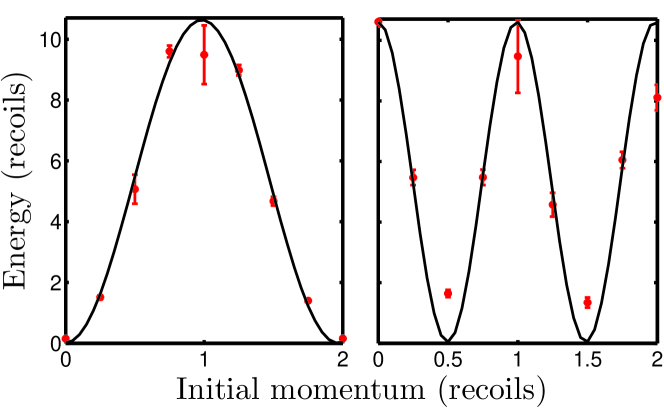
As discussed earlier, the AOKR dynamics can be examined by the observation of the energy or the variance of the momentum distribution in units of the recoil energy . In this section, we study how the energy of the system is influenced by taking into account the initial momentum of the atoms. The energy is scanned as a function of the initial momentum for different pulse periods for a number of kicks. In Fig. 14, the variation of the energy on the initial momentum for (left) and (right)
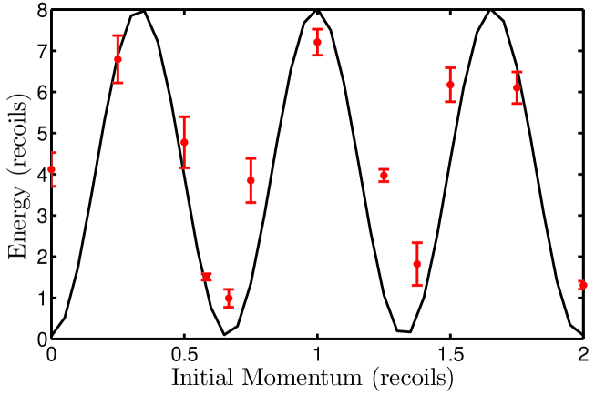
in both the experiment and simulation for two kicks is shown. For we see a strong peak in the energy at about . Similarly, for the resonant case oscillation in the energy is observed. These results are consistent with the results presented in Fig. 13. For , the energy varies at three times the rate for , as shown in Fig. 15. For the data points, the averaged profile is fitted to a number of Gaussians, one for each diffraction order, to obtain the energies after the kick sequence in each run. The standard deviation is then taken to estimate uncertainties in the results. A direct numerical variance of the velocity distribution was found to give similar results. Because of the sensitivity to small noise peaks at large momenta, these results were less consistent, and were therefore not used.
Next, the energy is examined as a function of the initial velocity for four kicks. As found, for a large number of kicks, the widths of quantum resonances when plotted as a function of kick period get smaller as the number of kicks get larger. Fig. 16 shows the energy as a function of the initial velocity for four kicks, for both the anti-resonance (left) and the resonance case (right). On the left, for there is an anti-resonance at zero momentum, yielding very small energies. There is a small maximum at an initial momentum of recoils, decreasing again close to zero at recoils. At an initial momentum of one recoil, there is a stronger maximum in the energy, decaying again to small energies at recoils before another smaller maximum. At initial momenta of two recoils, very small diffraction occurs and the energy returns to a small value close to zero. It should be noted that all these features, prominent in calculations, can be reproduced in the experiment.
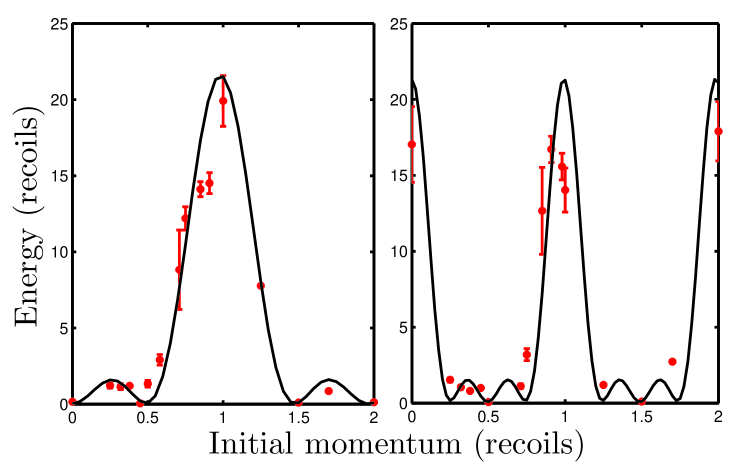
For the kick period corresponding to , a larger number of oscillations in energy in the simulation is observed. The maximum in these curves is observed to be much narrower than those for a small number of kicks. The maxima in the experiment is in agreement with that in the simulation, but the small-period oscillations in the simulation were not resolved in the experiment due to limited resolution for these settings.
IV.4 Details of the momentum distribution
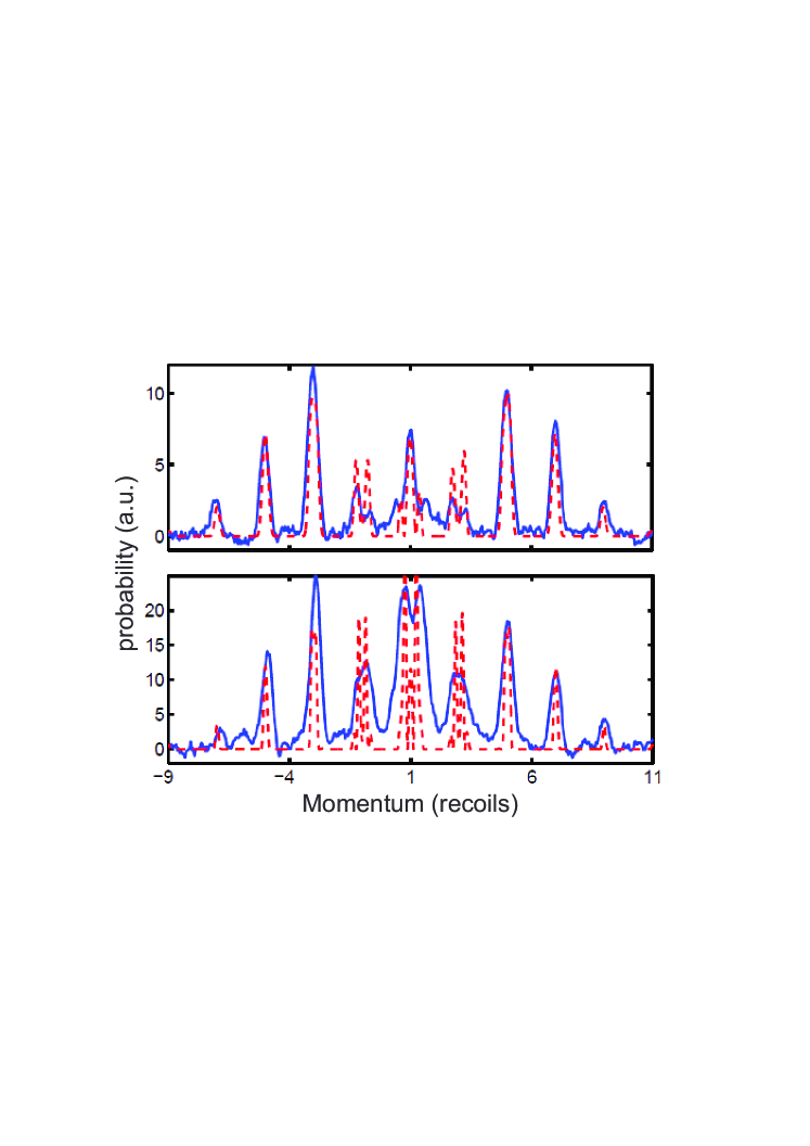
In a similar experiment, the momentum distributions obtained as a result of four kicks are shown in Fig. 17 for the antiresonance case (top) and the resonance case (bottom). A change in widths of the momentum distributions for different diffraction orders is observed in both cases. The observed difference in widths can easily be related to the separation of one velocity peak into multiple peaks in the simulation. For instance, the velocity peak at a momentum recoil is split into three, with varying heights in the two situations. This would be caused by the peak disappearing for recoils, and subsequently re-appearing for . In the final momentum distribution, the latter peaks appear even though they are not strongly weighted by the initial velocity distribution.
Similarly, the peaks at and recoils are split into two. This would be caused by the peaks appearing at a small . In addition,the peaks at recoils are found to be considerably narrower than the initial momentum distribution, which is caused by the fact that this diffraction peak only appears for very small . These observations can be verified in Fig. 11 by drawing a horizontal line at fixed and finding the diffraction orders. In the simulation, it has been found that the width of resonances as a function of the initial momentum gets smaller in the presence of a large number of kicks.
V Conclusions
In this paper we present an experimental study of quantum resonances in the kicked rotor system in detail. Quantum resonances are intrinsic to quantum mechanics and are therefore useful in studies related to the phenomenon of quantum chaos. We believe that the results provided in this paper contribute to a deeper understanding of quantum dynamics. Using the kinetic energy measurements, quantum resonances and antiresonances have been observed for a range of kicks in an AOKR experiment. In particular, we have shown how these resonances behave as we increase the number of kicks. For large number of kicks, the energy of the atom is very sensitive to each induced phase shift and is difficult to analyze accurately because of limited experimental resolution. Within the limits of experimental resolution we have found that these resonances get sharper as the number of kicks is increased, in good agreement with simulations. Moreover, higher order resonances that arise from fractional quantum revivals have been observed for pulse periods of (1/4) and (1/5) for five and ten kicks.
The study of quantum resonant effects in this work has been further extended to analyze the effect of the initial momentum of the atoms on quantum resonances in the AOKR. The first three quantum resonances have been examined for two and four kicks. A sinusoidal dependence of the energy on the initial momentum for two kicks has been observed. By increasing the number of kicks, the system becomes extremely sensitive to the initial momentum of the atoms. A more complex structure of the energy is observed for four kicks. For four kicks, the maxima in the experiment is in agreement with that in the simulation. The small-period oscillations in the simulations, however, were not resolved in the experiment due to limited resolution for these settings. The maximum in the energy curves is observed to be much narrower than those for small number of kicks, which is again in good agreement with simulations. With these experiments, it has been found that by applying a small frequency difference between the beams constituting the standing wave, we can dial any initial velocity we choose for the atoms with respect to the standing wave. In general, we found that the energy is periodic with initial momentum.
In the future it would be an interesting study to examine the dependence of the initial velocity of the atoms on the fractional resonant effects in the AOKR. In the “ballistic” regime, i.e. for the kick period close to one of the “quantum resonances”, a recent proposal McDowall et al. (2009) discusses the re-creation of the wave function by a strong, final pulse. The aim would be to confirm their predictions and investigate the influence of decoherence. In particular, it would be interesting to investigate the influence of the non-linearity caused by having a dense atom cloud. By manipulating the relative phase of the delta-kicks, a primitive “quantum computer” was recently demonstrated in Sadgrove et al. (2008). The aim would be to take this idea further, making use of the excellent control we have of the kick laser field. As these systems are very sensitive to initial conditions, the aim would be to investigate and measure these initial conditions, in particular to set an initial velocity and measure the recoil frequency, which is proportional to , where is the mass of the particle. This was outlined in a recent study Horne et al. (2011).
Acknowledgements.
The authors acknowledge the University of Auckland Research Fund for financial support. The authors would also like to thank Fabienne Haupert for her work on the initial setup. A. U. acknowledges the Higher Eduction Commission (HEC) of Pakistan for financial support.References
- Lichetenberg and Lieberman (1992) A. Lichetenberg and M. Lieberman, Regular and Chaotic Dynamics (Springer, New York, 1992).
- Lieberman and Lichtenberg (1972) M. A. Lieberman and A. J. Lichtenberg, Phys. Rev. A 5, 1852 (1972).
- Kornfeld et al. (1982) I. P. Kornfeld, S. V. Fomin, and Y. G. Sinai, Ergodic Theory (Springer, New York, 1982).
- Chirikov (1979) B. V. Chirikov, Phys. Rep 52, 263 (1979).
- Casati et al. (1979) G. Casati, B. V. Chirikov, J. Ford, and F. M. Izraeliv, Lecture Notes in Physics (Springer Berlin / Heidelberg, 1979).
- Chirikov et al. (1981) B. V. Chirikov, F. M. Izrailev, and D. L. Shepelyansky, Sov. Scient. Rev. C 2, 209 (1981).
- Shepelyanski (1983) D. L. Shepelyanski, Physica D. 8, 208 (1983).
- Moore et al. (1995) F. L. Moore, J. C. Robinson, C. F. Bharucha, B. Sundaram, and M. G. Raizen, Phys. Rev. Lett. 75, 4598 (1995).
- Ammann et al. (1998) H. Ammann, R. Gray, I. Shvarchuck, and N. Christensen, Phys. Rev. Lett. 80, 4111 (1998).
- Stöckmann (1999) H.-J. Stöckmann, Quantum Chaos: An Introduction (Cambridge University press, Cambridge, 1999).
- Fishman (1993) S. Fishman, in Quantum Chaos, edited by I. G. G. Casati and U. Smilansky (New-York North-Holland, 1993), p. 187.
- Izrailev and Shepelyansky (1980) F. M. Izrailev and D. L. Shepelyansky, Theor. Math. Phys. 43, 553 (1980).
- Izrailev (1980) F. M. Izrailev, Physica D. 1, 243 (1980).
- Saunders et al. (2007) M. Saunders, P. L. Halkyard, K. J. Challis, and S. A. Gardiner, Phys. Rev. A 76, 043415 (2007).
- Halkyard et al. (2008) P. L. Halkyard, M. Saunders, S. A. Gardiner, and K. J. Challis, Phys. Rev. A 78, 063401 (2008).
- Saunders et al. (2009) M. Saunders, P. L. Halkyard, S. A. Gardiner, and K. J. Challis, Phys. Rev. A 79, 023423 (2009).
- McDowall et al. (2009) P. McDowall, A. Hilliard, M. McGovern, T. Grünzweig, and M. F. Andersen, New. J. Phys. 11, 123021 (2009).
- Saif (2005) F. Saif, Phys. Rep 419, 207 (2005).
- Wimberger et al. (2003) S. Wimberger, I. Guarneri, and S. Fishman, Nonlinearity 16, 1381 (2003).
- Wimberger and Sadgrove (2005) S. Wimberger and M. Sadgrove, J. Phys. A 38, 10549 (2005).
- Deng et al. (1999) L. Deng, E. W. Hagley, J. Denschlag, J. E. Simsarian, M. Edwards, C. W. Clark, K. Helmerson, S. L. Rolston, and W. D. Phillips, Phys. Rev. Lett. 83, 5407 (1999).
- Oberthaler et al. (1999) M. K. Oberthaler, R. M. Godun, M. B. d’Arcy, G. S. Summy, and K. Burnett, Phys. Rev. Lett. 83, 4447 (1999).
- Szriftgiser et al. (2002) P. Szriftgiser, J. Ringot, D. Delande, and J. C. Garreau, Phys. Rev. Lett. 89, 224101 (2002).
- Duffy et al. (2004) G. J. Duffy, S. Parkins, T. Müller, M. Sadgrove, R. Leonhardt, and A. C. Wilson, Phys. Rev. E 70, 056206 (2004).
- Jones et al. (2007) P. H. Jones, M. Goonasekera, D. R. Meacher, T. Jonckheere, and T. S. Monteiro, Phys. Rev. Lett. 98, 073002 (2007).
- Wayper et al. (2007) S. A. Wayper, W. Simpson, and M. D. Hoogerland, Euro. Phys. Lett 79, 60006 (2007).
- Currivan et al. (2009) J. A. Currivan, A. Ullah, and M. D. Hoogerland, Euro. Phys. Lett 85, 30005 (2009).
- Ullah and Hoogerland (2011) A. Ullah and M. D. Hoogerland, Phys. Rev. E 83, 046218 (2011).
- Fishman et al. (1982) S. Fishman, D. R. Grempel, and R. E. Prange, Phys. Rev. Lett. 49, 509 (1982).
- Ryu et al. (2006) C. Ryu, M. F. Andersen, A. Vaziri, M. B. d’Arcy, J. M. Grossman, K. Helmerson, and W. D. Phillips, Phys. Rev. Lett. 96, 160403 (2006).
- Ovchinnikov et al. (1999) Y. B. Ovchinnikov, J. H. Müller, M. R. Doery, E. J. D. Vredenbregt, K. Helmerson, S. L. Rolston, and W. D. Phillips, Phys. Rev. Lett. 83, 284 (1999).
- Lepers et al. (2008) M. Lepers, V. Zehnlé, and J. C. Garreau, Phys. Rev. A 77, 043628 (2008).
- Talbot (1836) H. F. Talbot, Phil. Mag 9, 401 (1836).
- Saunders (2009) M. Saunders, Ph.D. thesis, Durham University (2009).
- Sadgrove (2005) M. P. Sadgrove, Ph.D. thesis, The University of Auckland (2005).
- Oskay et al. (2000) W. H. Oskay, D. A. Steck, V. Milner, B. G. Klappauf, and M. G. Raizen, Opt. Commun. 179, 137 (2000).
- Sadgrove et al. (2005) M. Sadgrove, T. Mullins, S. Parkins, and R. Leonhardt, Physica E. 29, 369 (2005).
- Wenas and Hoogerland (2008) Y. C. Wenas and M. D. Hoogerland, Review of Scientific Instruments 79, 053101 (2008).
- Reichl (1992) L. E. Reichl, The Transition to Chaos in Conservative Classical Systems: Quantum Manifestations (Springer-Verlag, Berlin, 1992).
- Berry et al. (2001) M. Berry, I. Marzoli, and W. Schleich, Physics world (2001).
- Sadgrove et al. (2007) M. Sadgrove, M. Horikoshi, T. Sekimura, and K. Nakagawa, Phys. Rev. Lett. 99, 043002 (2007).
- Dana et al. (2008) I. Dana, V. Ramareddy, I. Talukdar, and G. S. Summy, Phys. Rev. Lett. 100, 024103 (2008).
- Sadgrove et al. (2008) M. Sadgrove, S. Kumar, and K. Nakagawa, Phys. Rev. Lett. 101, 180502 (2008).
- Horne et al. (2011) R. A. Horne, R. H. Leonard, and C. A. Sackett, Phys. Rev. A 83, 063613 (2011).