Results from the 4PI Effective Action in 2- and 3-dimensions

Abstract

We consider a symmetric scalar theory with quartic coupling and solve the equations of motion from the 4PI effective action in 2- and 3-dimensions using an iterative numerical lattice method. For coupling less than 10 (in dimensionless units) good convergence is obtained in less than 10 iterations. We use lattice size up to 16 in 2-dimensions and 10 in 3-dimensions and demonstrate the convergence of the results with increasing lattice size. The self-consistent solutions for the 2-point and 4-point functions agree well with the perturbative ones when the coupling is small and deviate when the coupling is large.

I Introduction

The resummation of certain classes of Feynman diagrams to infinite loop order is a powerful method in quantum field theory. A well known example is the hard thermal loop theory Braaten1990 , developed in the context of thermal field theory, which resums all loop corrections which are of the same order as tree diagrams, when external momenta are soft.

In recent years, another kind of resummation approach, known as two-particle irreducible (2PI) effective action theory, has attracted a lot of attention. In the 2PI formalism, the effective action is expressed as a functional of the non-perturbative propagator Luttinger1960 ; Cornwall1974 , which is determined through a self-consistent stationary equation after the effective action is expanded to a certain order in the loop or $1/N$ expansion. This self-consistent equation of motion resums certain classes of diagrams to infinite order. The classes that are resummed are determined by the set of skeleton diagrams that are included in the truncated effective action. Numerical studies indicate that the 2PI effective action formalism is very successful in describing equilibrium thermodynamics, and also the quantum dynamics of far from equilibrium of quantum fields. The entropy of the quark-gluon plasma obtained from the 2PI formalism shows very good agreement with lattice data for temperatures above twice the transition temperature Blaizot1999 . The poor convergence problem usually encountered in high-temperature resummed perturbation theory with bosonic fields is also solved in the 2PI effective action theory Berges2005a . Furthermore, it has been shown that non-equilibrium dynamics with subsequent late-time thermalization can be well described in the 2PI formalism (see Berges2001 and references therein). The 2PI effective action has also been combined with the exact renormalization group to provide efficient non-perturbative approximation schemes Blaizot2011 . The shear viscosity in the $O(N)$ model has been computed using the 2PI formalism Aarts2004 .

The 2PI effective action theory has its own drawbacks and limitations. When the effective action is expanded to only 2-loops, the 2PI effective action is complete. However, when the expansion is beyond 2-loops, one must use a higher order effective theory to obtain a complete description Berges2004 . Higher order effective theories are defined in terms of self-consistently determined $n$-point functions for $n>2$. It has been shown that the 2PI effective action is insufficient to calculate transport coefficients for high temperature gauge theories Moore2002 ; Carrington2006 , but that higher order $n$PI effective actions can be used Carrington2008 .

The 4PI effective action for scalar field theories is derived in Ref. Norton1975 using Legendre transformations. The method of successive Legendre transforms is used in Carrington2004 ; Berges2004 . A new method has been developed to calculate the 5-loop 5PI and 6-loop 6PI effective action for scalar field theories Carrington2010 ; Carrington2011 . The 3PI and 4PI effective actions have been used to obtain a set of integral equations from which the leading order and next-to-leading order contributions to the viscosity can be calculated Carrington2009 ; Carrington2010b .

A lot of effort has been devoted to numerical computations in 2PI effective theories. For higher order $n$PI theories numerical calculations are extremely difficult and little progress has been made (see however Moore2012 ).

This paper is organized as follows. In section II we define our notation, in section III we present results from our numerical calculations in 2D and 3D, and in section IV we give our conclusions.

II General Formalism

We consider the following Lagrangian

$${\mathcal{L}}=\frac{1}{2}(\partial_{\mu}\varphi\partial^{\mu}\varphi-m^{2}{\varphi}^{2})-\frac{i\lambda}{4!}\varphi^{4}\,.$$ (1)

The classical action is:

$$S[\phi]=S_{0}[\varphi]+S_{\mathrm{int}}[\varphi]\,,$$ (2)

$$S_{0}[\varphi]=\frac{1}{2}\int d^{d}x\,d^{d}y\,\varphi(x)\big{[}iG_{0}^{-1}(x-y)\big{]}\varphi(y)\,,$$

$$S_{\mathrm{int}}[\varphi]=-\frac{i\lambda}{4!}\int d^{d}x\varphi^{4}(x)\,.$$

In most equations in this paper, we suppress the arguments that denote the space-time dependence of functions. As an example of this notation, the non-interacting part of the classical action is written:

$$S_{0}[\varphi]=\frac{1}{2}\int d^{d}x\,d^{d}y\,\varphi(x)\big{[}iG_{0}^{-1}(x-y)\big{]}\varphi(y)~{}~{}\rightarrow~{}~{}\frac{i}{2}G_{0}^{-1}\varphi^{2}\,,$$ (3)

$$G_{0}^{-1}=-i\frac{\delta^{2}S_{cl}[\varphi]}{\delta\varphi^{2}}\bigg{|}_{\varphi=0}=i(\Box+m^{2})\,.$$

The effective action is obtained from the Legendre transformation of the connected generating functional:

$$Z[R_{1},R_{2},R_{3},R_{4}]=\int[d\varphi]\;{\rm Exp}[i\,(S_{cl}[\varphi]+R_{1}\varphi+\frac{1}{2}R_{2}\varphi^{2}+\frac{1}{3!}R_{3}\varphi^{3}+\frac{1}{4!}R_{4}\varphi^{4})]\,,$$ (4)

$$W[R_{1},R_{2},R_{3},R_{4}]=-i\,{\rm Ln}Z[R_{1},R_{2},R_{3},R_{4}]\,,$$

$$\Gamma[\phi,G,V_{3},V_{4}]=W-R_{1}\frac{\delta W}{\delta R_{1}}-R_{2}\frac{\delta W}{\delta R_{2}}-R_{3}\frac{\delta W}{\delta R_{3}}-R_{4}\frac{\delta W}{\delta R_{4}}\,.$$

Connected and proper Green functions are denoted $V_{j}^{c}$ and $V_{j}$ respectively, where the subscript $j$ indicates the number of legs. They are defined:

$$V_{j}^{c}=\langle\varphi^{j}\rangle_{c}=-(-i)^{j+1}\frac{\delta^{j}W}{\delta R_{1}^{j}}\,,$$ (5)

$$V_{j}=i\frac{\delta^{j}}{\delta\phi^{j}}\Gamma_{\rm 1PI}=i\frac{\delta^{j}}{\delta\phi^{j}}\left(W[R_{1}]-R_{1}\phi\right)\,.$$ (6)

The equations that relate the connected and proper vertices are obtained from their definitions using the chain rule. We organize the calculation of the effective action using the method of subsequent Legendre transforms Carrington2004 ; Berges2004 . This method involves starting from an expression for the 2PI effective action and exploiting the fact that the source terms $R_{3}$ and $R_{4}$ can be combined with the corresponding bare vertex by defining a modified interaction vertex. The result is:

$$\Gamma[\phi,G,V_{3},V_{4}]=\frac{i}{2}G_{0}^{-1}\phi^{2}+\frac{i}{2}\mathrm{Tr}\ln G^{-1}+\frac{i}{2}\mathrm{Tr}G^{-1}_{0}G+\Gamma_{\mathrm{int}}[\phi,G,V_{3},V_{4}]\,,$$ (7)

$$i\Gamma_{\rm int}[\phi,G,V_{3},V_{4}]=\frac{\lambda}{4!}\phi^{4}+\frac{\lambda}{4}(\phi^{2}G)+\Phi_{2}[\phi,G,V_{3},V_{4}]\,,$$

where $\Phi_{2}[\phi,G,V_{3},V_{4}]$ represents diagrams with 2 and more loops. In this paper we consider only the self-consistent 2- and 4-point functions in the symmetric phase. These are obtained by solving simultaneously the equations of motion:

$$\frac{\delta\Gamma[\phi,G,V_{3},V_{4}]}{\delta G}\bigg{|}_{\phi=0,G=\tilde{G},V_{3}=0,V_{4}=\tilde{V}_{4}}=0\,,~{}~{}~{}\frac{\delta\Gamma[\phi,G,V_{3},V_{4}]}{\delta V_{4}}\bigg{|}_{\phi=0,G=\tilde{G},V_{3}=0,V_{4}=\tilde{V}_{4}}=0\,.$$ (8)

From now on we drop the subscript on the 4-point vertex function and write $V:=V_{4}$ and $\tilde{V}:=\tilde{V}_{4}$.

The variables $m$, $\lambda$, $G$ and $V$ in section II should all carry a subscript $B$ to indicate that they are bare quantities. These bare quantities (with subscript $B$) are related to the renormalized ones by the following relations:

$$\delta m^{2}=Zm_{B}^{2}-m^{2}\,,~{}~{}\delta\lambda=Z^{2}\lambda_{B}-\lambda\,,$$ (9)

$$G_{B}=ZG\,,~{}~{}V_{B}=Z^{-2}V\,,$$

$$ZG^{-1}_{0B}=G^{-1}_{0}+\delta G^{-1}_{0}\,,~{}~{}~{}\delta G^{-1}_{0}=i(\delta Z\Box+\delta m^{2})\,,~{}~{}~{}\delta Z=Z-1\,.$$

In order to simplify the notation we have not introduced a subscript $R$ for renormalized quantities and we have suppressed the subscript $B$ everywhere except in the equation (9). All quantities in section II are bare, and all quantities in the following sections are renormalized.

We divide the functional $\Phi_{2}[G,V]$ into two pieces: terms without counter-terms or bare vertices, and terms that do contain either counter-terms or bare vertices. We denote these two pieces $-i\Phi_{\mathrm{int}}[G,V]$ and $-i\Phi_{0}[G,V]$, respectively. Using this notation we write the effective action in equation (7) as:

$$i\Gamma[G,V] =-\frac{1}{2}\mathrm{Tr}\ln G^{-1}-\frac{1}{2}\mathrm{Tr}G^{-1}_{0}G+\Phi_{0}[G,V]+\Phi_{\mathrm{int}}[G,V]\,,$$ (10)

$$\Phi_{0} =-\frac{1}{2}\mathrm{Tr}\delta G^{-1}_{0}G+\frac{1}{8}(\lambda+\delta\lambda)G^{2}+\frac{1}{4!}(\lambda+\delta\lambda)G^{4}V\,.$$

The functional $\Phi_{0}$ has the same form for $n\geq 4$ and all orders in the loop expansion and $\Phi_{\mathrm{int}}$ contains a set of skeleton diagrams which are determined by the orders of the Legendre transform and loop expansion. The sum $\Phi_{2}=\Phi_{0}+\Phi_{\mathrm{int}}$ is shown to 4-loops in figure 1. In all diagrams, bare 4-vertices are represented by white circles, counter-terms are circles with crosses in them, and solid dots are the vertex $V$.

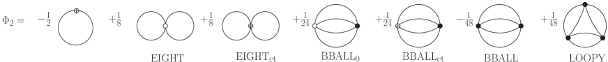
Figure 1: The effective action at 4-Loops including counter-terms. The open circle is a bare vertex, the circle with a cross denotes a counter-term, and the vertex $V$ is indicated by a solid dot.

The equation of motion for $V$ is obtained from the variational equation $\delta\Gamma/\delta V=0$ (see equation (8)). Using the 4-Loop 4PI effective action gives the result in figure 2 and equation (II). We use throughout the notation $dQ=d^{d}q/(2\pi)^{d}$.

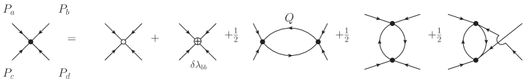
Figure 2: Self-consistent equation of motion for the proper 4-point vertex.

$$V(P_{a},P_{b},P_{c}) =\lambda+\delta\lambda+V_{s}(P_{a},P_{b},P_{c})+V_{t}(P_{a},P_{b},P_{c})+V_{u}(P_{a},P_{b},P_{c})\,,$$

$$V_{s}(P_{a},P_{b},P_{c}) =\frac{1}{2}\int dQ\;V(P_{a},P_{c},Q)G(Q)G(Q+P_{a}+P_{c})V(P_{b},P_{d},-Q)\,,$$ (11)

$$V_{t}(P_{a},P_{b},P_{c}) =V_{s}(P_{a},P_{c},P_{b})\,,$$

$$V_{u}(P_{a},P_{b},P_{c}) =V_{s}(P_{a},P_{b},P_{d})\,,~{}~{}~{}P_{d}=-(P_{a}+P_{b}+P_{c})\,.$$

The equation of motion for the 2-point function is obtained from the variational equation $\delta\Gamma/\delta G=0$ (see equation (8)). It has the form of a Dyson equation where the self-energy is proportional to the functional derivative of the terms in the effective action with two and more loops:

$$G^{-1}=G_{0}^{-1}-\Sigma\,,~{}~{}\Sigma=2\frac{\delta\Phi_{2}}{\delta G}\,.$$ (12)

The result is shown in the first line of figure 3. The diagrams can be rearranged by substituting the $V$ equation of motion into the vertex on the left side of the sixth diagram. This substitution cancels the 3-loop diagram and produces the result in the second line of the figure and equation (13).

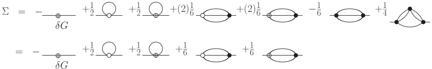
Figure 3: The self-energy obtained from equations (10) and (12).

$$\Sigma(p) = i(\delta ZP^{2}-\delta m^{2})+\frac{1}{2}(\lambda+\delta\lambda)\int dQ\;G(Q)$$ (13)

$$+\,\frac{1}{6}(\lambda+\delta\lambda)\int dQ\int dK\;V(P,Q,K)G(Q)G(K)G(Q+K+P)\,.$$

Numerical calculations will be done in Euclidean space and therefore we redefine the variables:

$$q_{0}=iq_{E}\,,~{}~{}\delta Z=\delta Z_{E}\,,~{}~{}\delta m^{2}=\delta m^{2}_{E}\,,~{}~{}G=-iG_{E}\,,~{}~{}\Sigma=-i\Sigma_{E}\,,$$ (14)

$$\lambda=-i\lambda_{E}\,,~{}~{}\delta\lambda=-i\delta\lambda_{E}\,,~{}~{}V=iV_{E}\,.$$

The Dyson equation in Euclidean space is (see equation (12)):

$$G_{E}^{-1}(P)=G^{-1}_{0E}(P)+\Sigma_{E}(P)\,.$$ (15)

All variables from here on are Eucledian and we suppress the subscript $E$. The coupling constant and 4-point vertex have dimension $4-d$ so that in 2D $\lambda\sim m^{2}$ and in 3D $\lambda\sim m$. We work in mass units, in which all dimensional quantities are scaled by the mass.

III Numerical Results

III.1 Perturbative Theory

We start by looking at the perturbative theory. For the 4-point function at the 1-loop level the diagrams we need are obtained from figure 2 with lines and proper vertices replaced by bare ones. In less than 4-dimensions there are no ultraviolet divergences and from equation (II) we find:

$$V(P_{a},P_{b},P_{c}) = -\lambda-\delta\lambda+\frac{\lambda^{2}}{2}\frac{\Gamma(2-d/2)}{(4\pi)^{d/2}}\int_{0}^{1}dx\bigg{\{}\frac{1}{\big{[}m^{2}+x(1-x)(P_{a}+P_{c})^{2}\big{]}^{2-d/2}}$$ (16)

$$+\frac{1}{\big{[}m^{2}+x(1-x)(P_{a}+P_{b})^{2}\big{]}^{2-d/2}}+\frac{1}{\big{[}m^{2}+x(1-x)(P_{b}+P_{c})^{2}\big{]}^{2-d/2}}\bigg{\}}\,.$$

To obtain the 2-point function at 2-Loops we need to calculate the tadpole and sunset diagrams in equation (13) with lines and proper vertices replaced by bare ones. We use dimensional regularization and define $\epsilon=1-d/2$. The tadpole diagram is momentum independent in any number of dimensions. In 3D it is finite using dimensional regularization and in 2D the divergent part is easily obtained as $\lambda/(8\pi\epsilon)$. The sunset contribution to the self-energy is:

$$\Sigma^{\rm 2~{}dims}_{\rm sunset}(P)=-\frac{\lambda^{2}}{6(4\pi)^{2}}\int_{0}^{1}dx\int_{0}^{1}dy\frac{1}{[y+(1-y)x(1-x)]m^{2}+y(1-y)x(1-x)P^{2}}\,.$$ (17)

$$\Sigma^{\rm 3~{}dims}_{\rm sunset}(P)=-\frac{\lambda^{2}}{6}\frac{\Gamma(\epsilon)}{(4\pi)^{3-2\epsilon}}\int_{0}^{1}\frac{dx}{(x(1-x))^{1/2+\epsilon}}\int_{0}^{1}\frac{dy\,y^{\epsilon-1/2}}{[P^{2}y(1-y)+m^{2}(1-y+\frac{y}{x(1-x)})]^{\epsilon}}\,.$$

The integral is finite in 2D. In 3D the divergence is momentum independent. We can write the divergent part of the self-energy as:

$$\Sigma^{\rm div}=\frac{\lambda}{8\pi}\,\frac{1}{\epsilon}\delta_{d2}-\frac{1}{\epsilon}\frac{\lambda^{2}}{12(4\pi)^{2}}\delta_{d3}\,,$$ (18)

where the Kronecker deltas indicate which pieces contribute in 2D and 3D. Thus we have that in 2D the tadpole has a momentum independent divergence and the sunset diagram is finite, while in 3D the situation is reversed and the sunset has a momentum independent divergence but the tadpole is finite. Using Pauli-Villars regularization the tadpole has a momentum independent divergence in 2D or 3D and the sunset has a momentum independent divergence in 3D only. In all cases, the counter-term $\delta m^{2}$ completely removes the divergence and we can set $\delta Z=0$. We use the renormalization condition $\Sigma(0)=0$ to determine the mass counter-term. Since the tadpole diagram is independent of the external momentum (in any dimension), this renormalization condition completely removes the entire tadpole contribution, and we can just drop the diagram. In both 2D and 3D the 4-vertex does not UV-renormalize and the natural choice is to set $\delta\lambda=0$, so that $\lambda$ is defined as the limit of the 4-point function at large external momenta.

III.2 Non-perturbative calculation

The diagrams produced by expanding the $n$PI equation of motion are not the same as those produced by the perturbative expansion, some diagrams appear with different symmetry factors, and some diagrams are missing altogether. In less than 4-dimensions however, the only fundamental divergences are the tadpole and sunset diagrams, and each insertion of a bare self-energy is accompanied by the mass counter-term that makes it finite. Iteration does not create new sub-divergences and therefore iterations amount to inserting renormalized self-energies, without introducing new divergences. Therefore one can also renormalize the non-perturbative theory using only a mass counter-term. In order to compare the non-perturbative results with the perturbative ones, we use the same renormalization conditions.

To obtain non-perturbative results we solve the self-consistent equation of motion for the 2- and 4-point functions using a numerical lattice method. We use an $N^{d}$ symmetric lattice with periodic boundary conditions. The size of the lattice is limited by the calculation time and memory constraints. In 2D we use $N$ up to 16 and in 3D $N$ up to 10. The lattice spacing is $a$ and we choose $a=2\pi/(Nm)$. In Euclidean space, each momentum component is discretized:

$$p_{i}=\frac{2\pi}{aN}n_{i}\,,\quad n_{i}=-\frac{N}{2}+1,...,\frac{N}{2}\,,$$ (19)

and the periodic boundary conditions take the form $n_{i}+N=n_{i}$ for all momentum components. The lattice momenta given by equation (19) form a Brillouin zone. On the lattice, the equation of motion for the 4-point vertex (equation (II)) is transformed into:

$$V(P_{a},P_{b},P_{c}) = -\lambda-\delta\lambda+\frac{1}{2}\frac{1}{(aN)^{d}}\sum_{Q}\Big{[}V(P_{a},P_{c},Q)G(Q)G(Q+P_{a}+P_{c})V(P_{b},P_{d},-Q)$$ (20)

$$+V(P_{a},P_{b},Q)G(Q)G(Q+P_{a}+P_{b})V(P_{c},P_{d},-Q)$$

$$+V(P_{a},P_{d},Q)G(Q)G(Q+P_{a}+P_{d})V(P_{b},P_{c},-Q)\Big{]}\,,$$

and the 2-loop self-energy (equation (13)) is:

$$\Sigma(P) = \delta Z\,P^{2}+\delta m^{2}+\frac{1}{6}(\lambda+\delta\lambda)\frac{1}{(aN)^{2d}}\sum_{Q}\sum_{K}V(P,Q,K)G(Q)G(K)G(Q+K+P)\,.$$ (21)

We start from an initial 4-point vertex and propagator which we chose to be the bare vertex and free propagator. Then we use equations (15), (20) and (21) and simultaneously search for self-consistent solutions using an iterative procedure. In order to make the iterations converge more quickly, we adopt the following formula to update the vertex and propagator at every iteration Berges2005a :

$$V_{\mathrm{update}} = \alpha V_{\mathrm{new}}+(1-\alpha)V\,,$$ (22)

$$G_{\mathrm{update}} = \alpha G_{\mathrm{new}}+(1-\alpha)G\,,$$ (23)

where $\alpha$ is the convergence factor, and we choose $\alpha=0.8$.

In all of our calculations, the full momentum dependence of the vertex and self-energy is taken into account. In order to produce figures, we must fix some momentum components to obtain a 2-dimensional representation of the results. For the 4-point function, when we consider the dependence on either the number of iterations or the coupling, we choose all momentum components equal to zero. We also study the momentum dependence of the 4-point function as a function of $(p_{a})_{x}$ and $\{(p_{a})_{x},(p_{b})_{x}\}$ with all other momentum components set to zero, where $(p_{a})_{x}$ and $(p_{b})_{x}$ are the $x$-components of the momentum of the first and second legs. For the 2-point function, because of the renormalization condition, we consider $\Sigma(p_{x}=2,0,0)$ as a function of the number of iterations and coupling, and also $\Sigma(p_{x},0,0)$ at fixed coupling.

It is interesting to compare the results we obtain from the non-perturbative calculation with the corresponding perturbative ones. The continuum perturbative solution can be obtained from equations (16) and (17). In order to check our equations, we also do the perturbative calculation on the lattice by solving equations (20) and (21) with the the self-consistent vertex and propagator replaced by the bare ones. We work in 3D and use $N=6$, 8, 10, 12 and 30, the results are shown in figure 4. For very large $N$ the lattice calculation converges to the continuum limit, as it should. In this paper we do not go beyond $N=10$, and although it is clear that larger $N$’s are desirable, the figure shows that the calculation converges in the sense that $N=10$ is closer to $N=8$ than $N=8$ is to $N=6$. Later in this section we discuss convergence further.

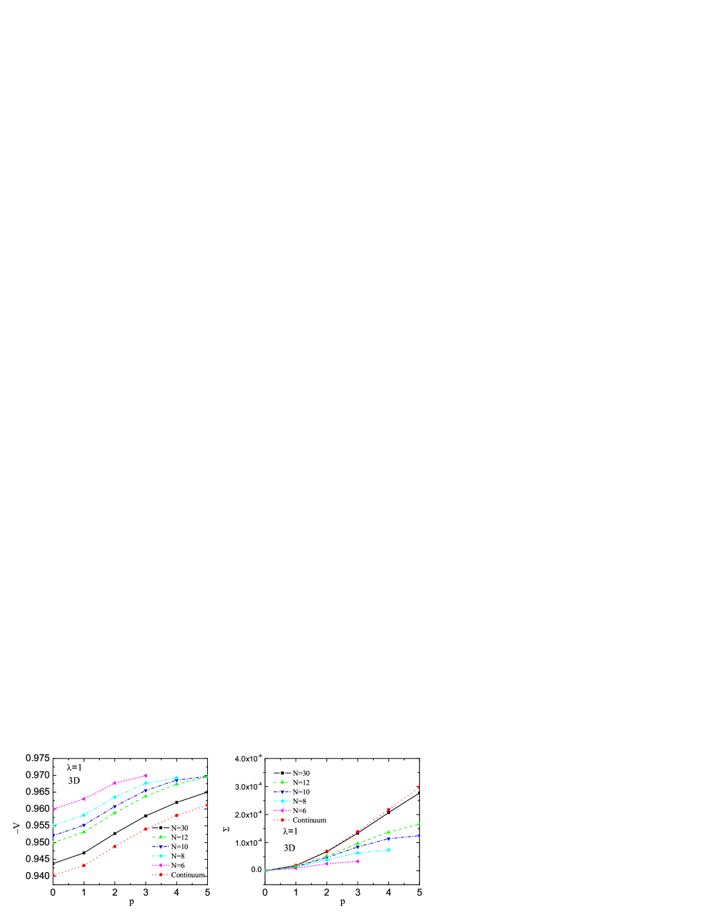
Figure 4: The perturbative vertex and self-energy from the lattice calculation with $N=6$, 8, 10, 12 and 30, and in the continuum limit.

In figure 5 we show the 4-point function and self-energy as a function of the number of iterations. We choose $\lambda=5$ (in mass units), and $N=16$ in 2D and $N=8$ in 3D. The first two iterations are not included so that the evolution can be seen more clearly. In both the 2D and 3D cases, self-consistent convergent solutions are obtained quickly after several iterations. The number of iterations that is needed increases slightly as $\lambda$ increases, but it is easy to obtain converged solutions for $\lambda\sim 10$.

Figure 5: The 4-point vertex and self-energy as a function of the number of iterations for $\lambda=5$, and $N=16$ for 2D and $N=8$ for 3D.

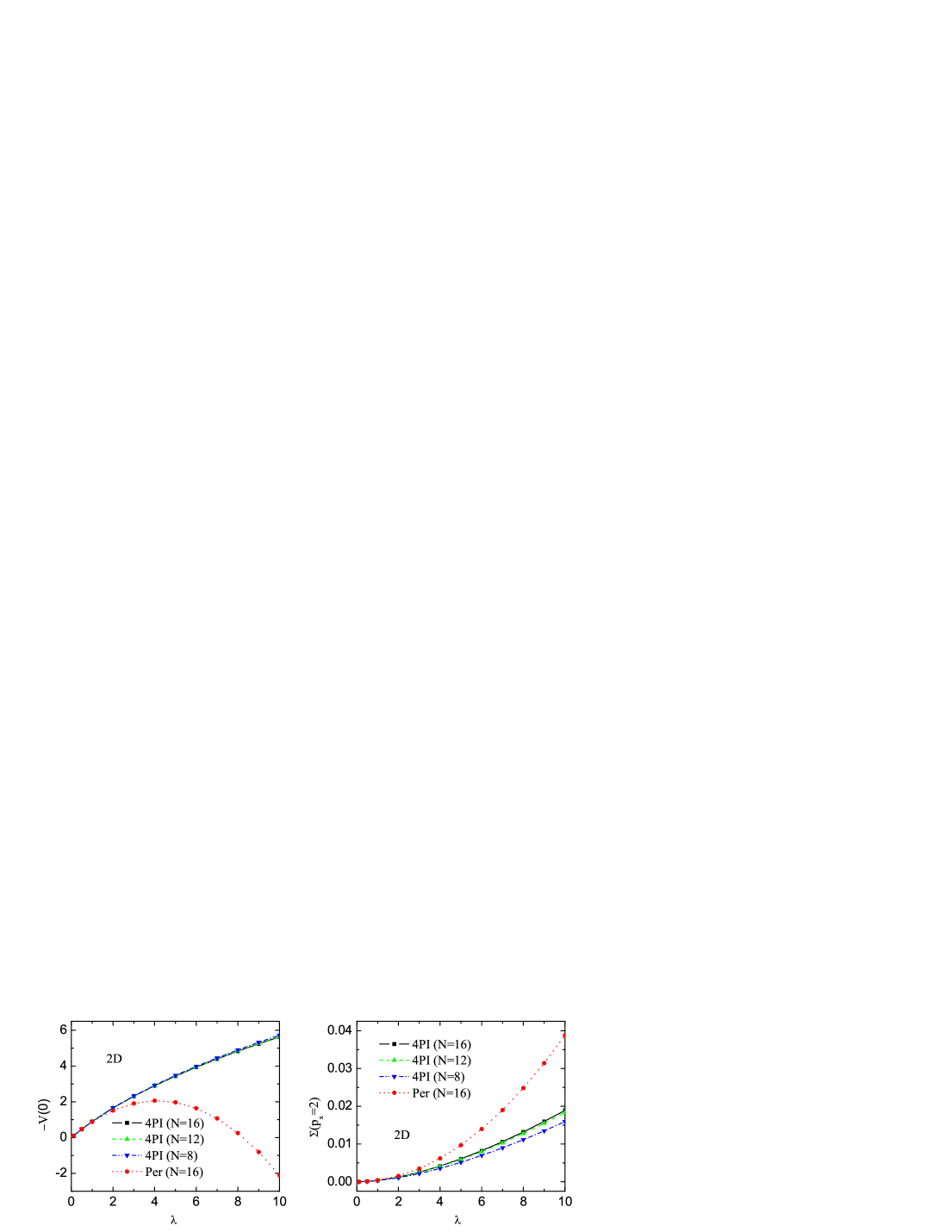
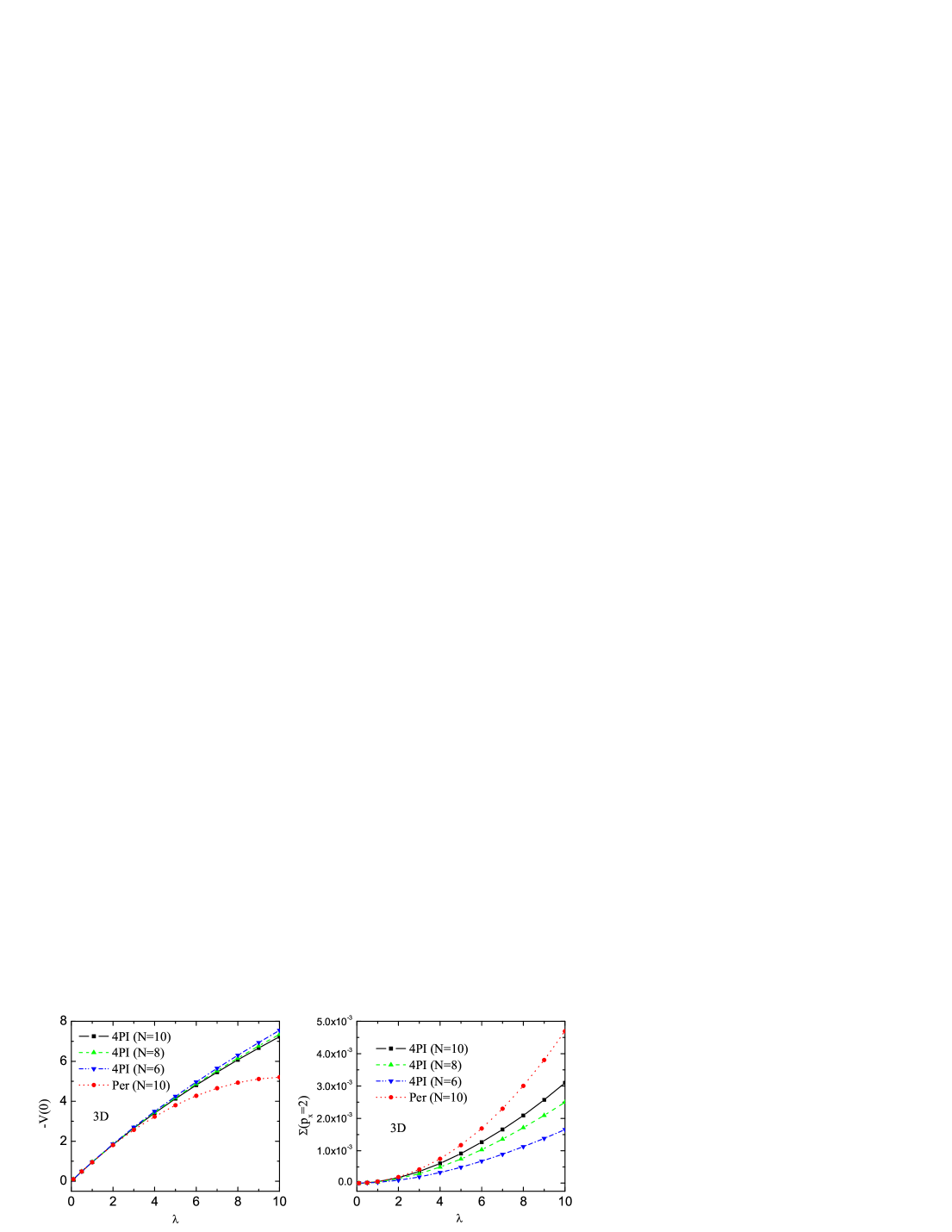
Figure 6: Comparison of the 2D and 3D 4-point vertex and self-energy as functions of the coupling strength $\lambda$. The 4PI calculations are done in 2D with $N=16,12$ and 8, and in 3D with $N=10,8$ and 6. The top left panel is the 2D 4-vertex, top right is the 2D self-energy, bottom left is the 3D 4-vertex, bottom right is the 3D self-energy. In each graph the perturbative result is the dotted line which joins the round markers (red on-line).

Figure 6 shows the 2D and 3D 4-point vertex and self-energy as functions of the coupling strength $\lambda$, calculated from 4PI effective action and perturbation theory. In all cases the non-perturbative results agree well with the perturbative ones when the coupling strength is small. When the coupling constant becomes large the 4PI results differ significantly from the perturbative ones, indicating the importance of a non-perturbative method in the strong coupling regime. In 2D, the results for the 4PI vertex are almost independent of the lattice number $N$. The self-energy depends more strongly on the lattice size but converges well when $N$ is increased to 16 (the curve corresponding to $N=16$ almost coincides with that corresponding to $N=12$). In 3D, calculations can only be performed up to $N=10$ because the three independent external momenta of the 4-point vertex consume lot of computational resource. Convergence is good for the 4-point vertex, but the results for the self energy have a stronger dependence on the lattice number.

In order to investigate whether convergence is obtained with $N=10$, we look at the ratios of the vertex and self energy calculated with $N=8$ and $N=10$, and with $N=6$ and $N=8$. The results are shown in Fig. 7. The fact that these ratios approach 1 indicates that our results are converging.

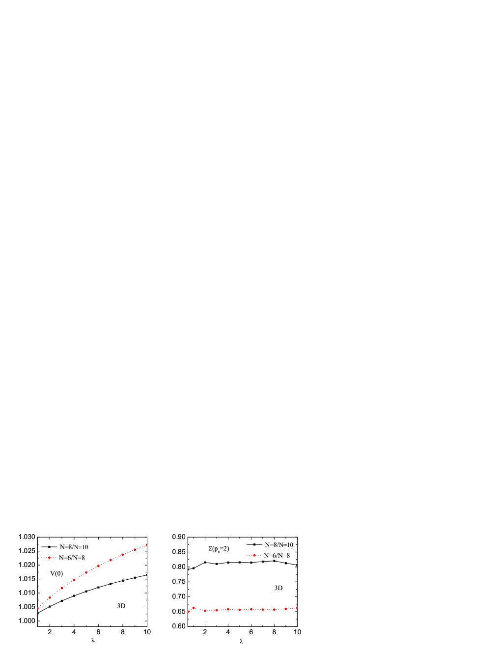
Figure 7: Non-perturbative results for $V_{N=8}/V_{N=10}$, $V_{N=6}/V_{N=8}$, $\Sigma_{N=8}/\Sigma_{N=10}$ and $\Sigma_{N=6}/\Sigma_{N=8}$ in 3D as functions of the coupling strength $\lambda$.

Figure 8 shows the dependence of the 4-point vertex on the first momentum component in 2D and 3D, choosing all momentum components other than $(p_{a})_{x}$ zero and using the coupling strength $\lambda$ equal to 1 and 5. We choose $N=16,12$ and 8 for the 2D calculations, and $N=10,8$ and 6 for the 3D ones. The difference between the non-perturbative vertex and the perturbative one is greater when the coupling constant is larger, as expected.The momentum dependence is produced by the 1-loop diagram and at large momentum the 4-point vertex scales as $-V\sim\lambda-Cp^{d-4}$, as expected. The results obtained by increasing the lattice number converge in both 2D and 3D.

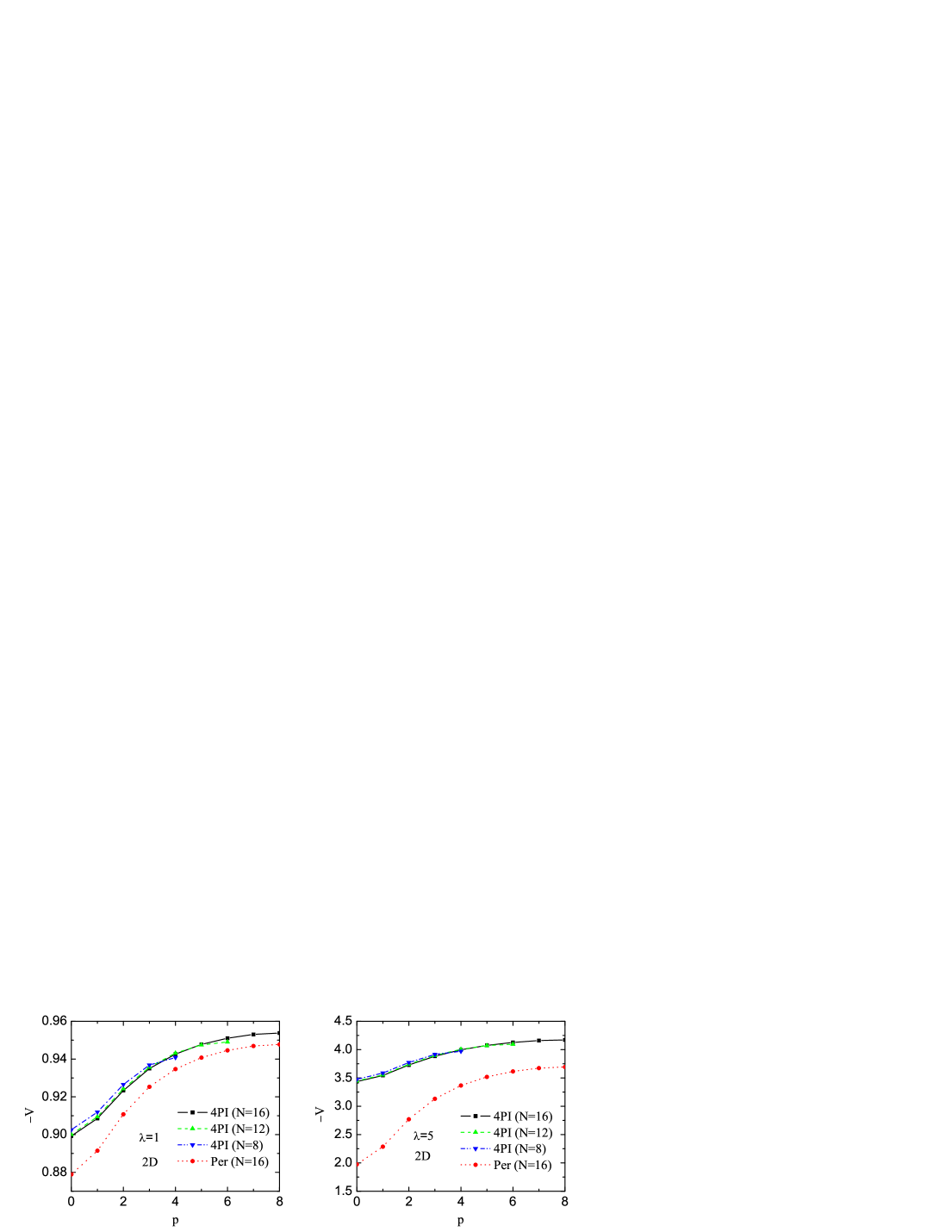
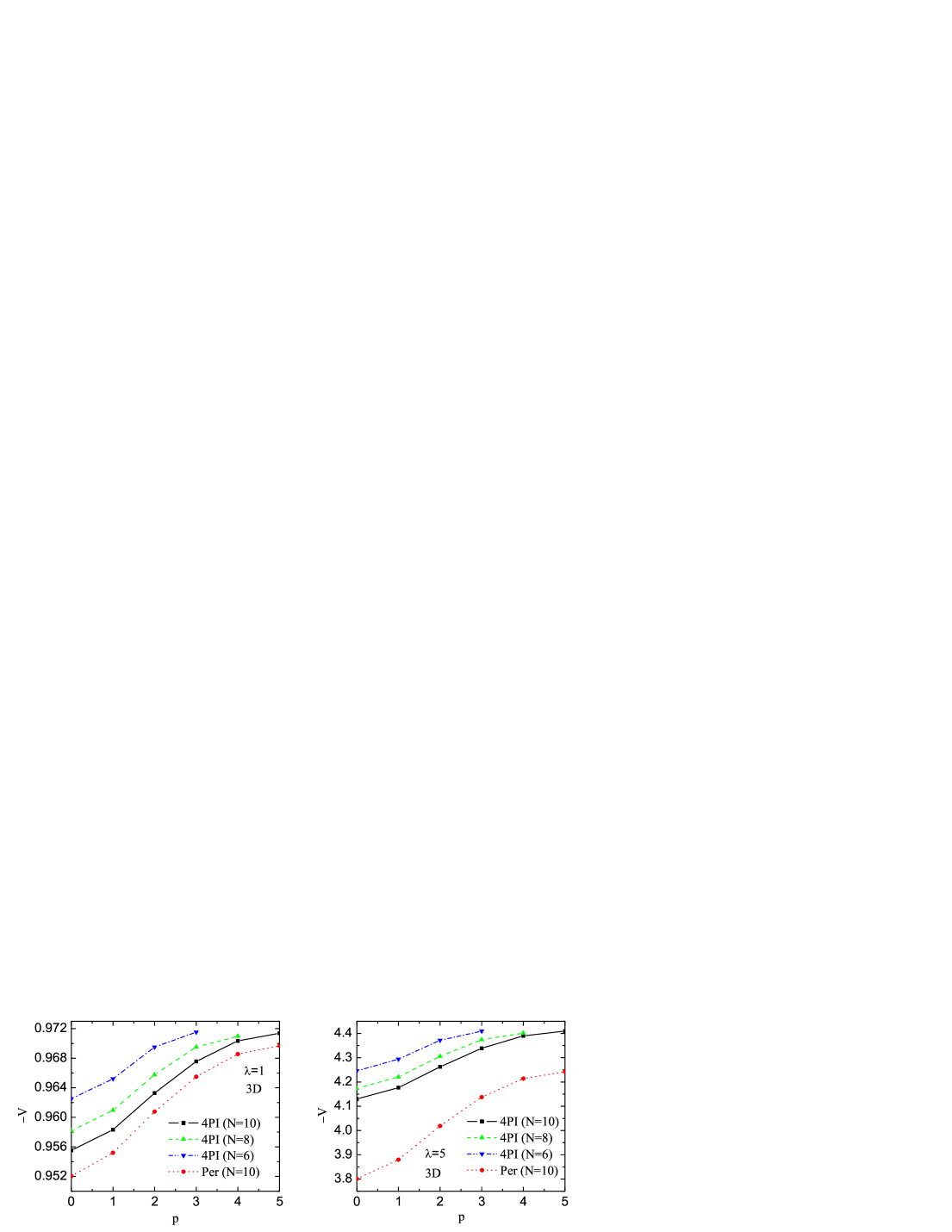
Figure 8: Dependence of the 2D and 3D 4-point vertex on $(p_{a})_{x}$ with all other external momenta components set to zero. Top left panel is 2D with $\lambda=1$, top right is 2D with $\lambda=5$, bottom left is 3D with $\lambda=1$, and bottom right is 3D with $\lambda=5$. The 4PI calculations are done in 2D with $N=16,12$ 8, and in 3D with $N=10,8$ and 6. The perturbative result is the dotted line which joins the round markers (red on-line).

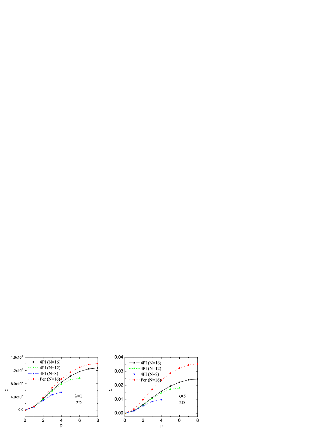
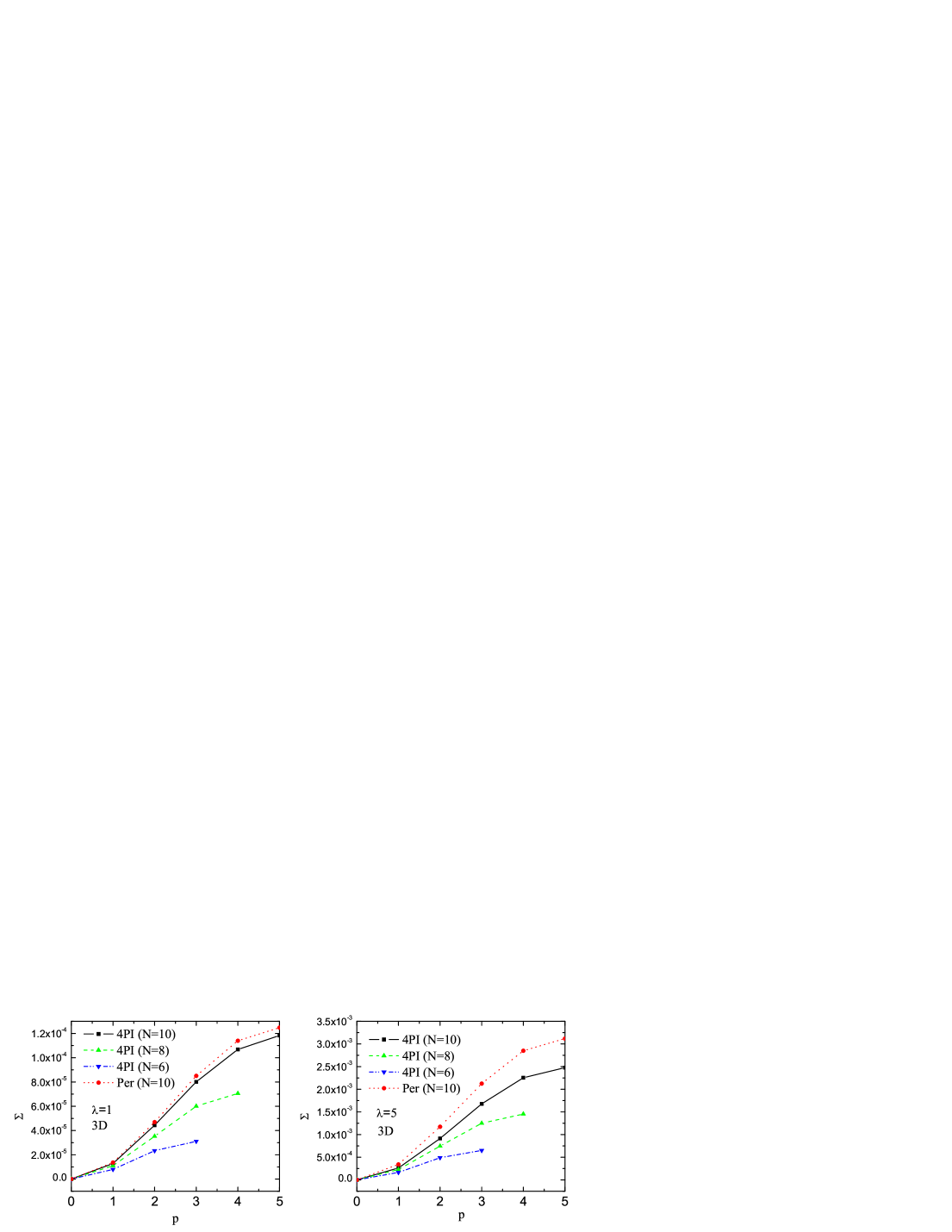
Figure 9: Dependence of the 2D and 3D self-energy on the $p_{x}$ with all other momentum components set to zero. Top left panel is 2D with $\lambda=1$, top right is 2D with $\lambda=5$, bottom left is 3D with $\lambda=1$, and bottom right is 3D with $\lambda=5$. The 4PI calculations are done in 2D with $N=16,12$ 8, and in 3D with $N=10,8$ and 6. The perturbative result is the dotted line which joins the round markers (red on-line).

In figure 9 we show the dependence of the self-energy on $p_{x}$ with all other momentum components zero. The momentum dependence comes from the sunset diagram and at large momentum the self-energy scales like $C-C^{\prime}/p^{2}$ in 2D and $C+C^{\prime}{\rm log}(p)$ in 3D, as expected. The difference between the non-perturbative self energy and the perturbative one is greater when the coupling constant is larger. Convergence with increasing lattice size is not as good as for the vertex, and not as good in 3D as in 2D. However, the analysis in figure 7 indicates that our results are converging.

It is interesting to compare the 4PI 2-point function with the 2PI version, which is obtained from equation (21) with the self-consistent vertex replaced by the bare one. For the values of $\lambda$ chosen in figure 9 the 2PI result is almost identical to the perturbative one, and it is only for very large values of $\lambda$ that one can see the difference. We illustrate this point in figure 10 where we show the perturbative, 2PI and 4PI self-energies for $\lambda=5$ and 50, and $N=8$.

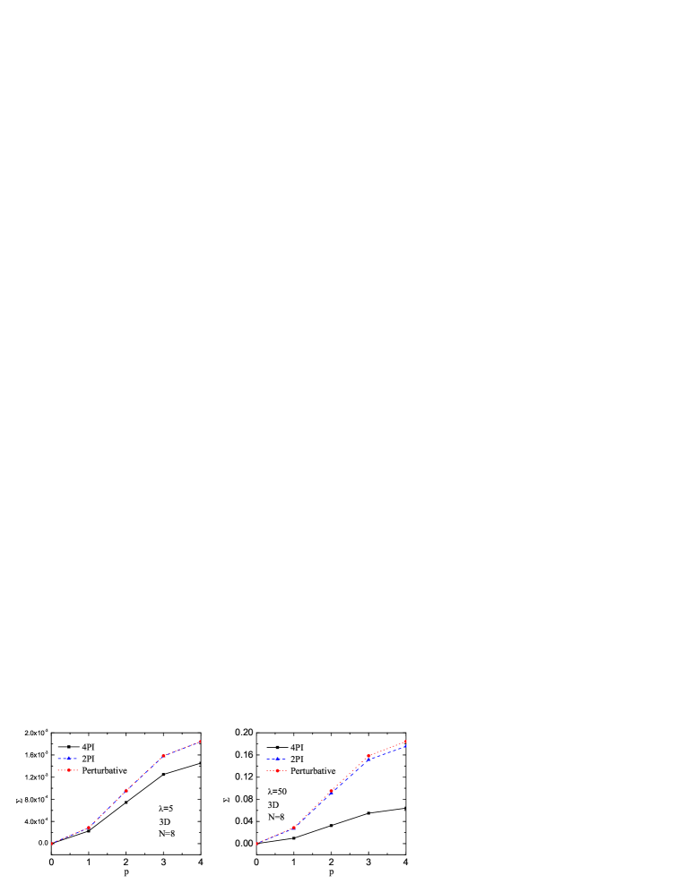
Figure 10: Comparison of the 3D perturbative, 2PI and 4PI self-energies for $\lambda=5$ and $\lambda=50$, with $N=8$.

In figure 11 we give contour plots of the 2D and 3D 4-point vertex which show the dependence of the vertex on the two momentum components $(p_{a})_{x}$ and $(p_{b})_{x}$ with all others chosen to be zero. The vertex has a minimum at the origin of the coordinates, and the gradient varies with direction.

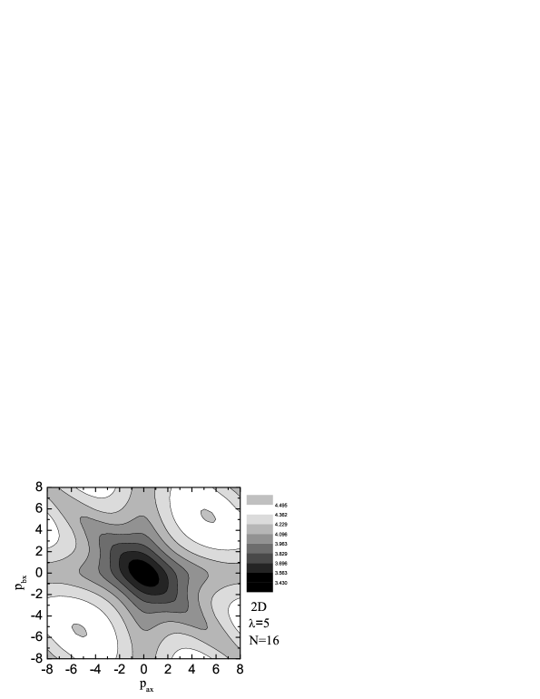
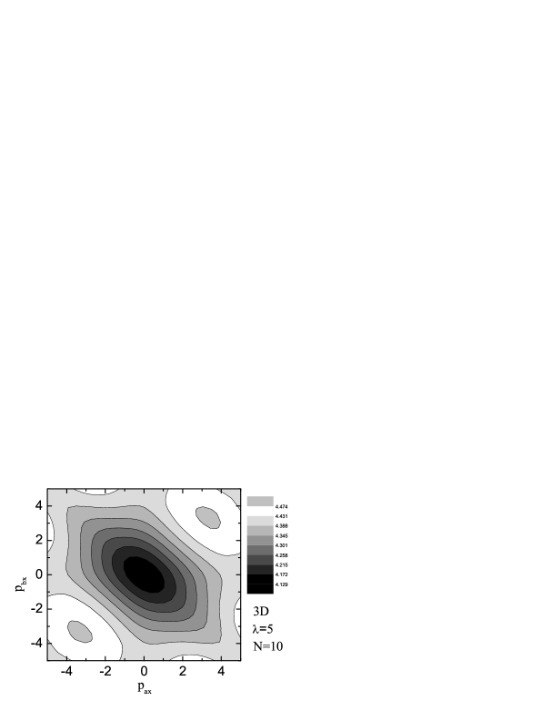
Figure 11: Contour plot of the 4-point vertex in 2D and 3D as a function of $(p_{a})_{x}$ and $(p_{b})_{x}$ with all other momenta components set to zero for $\lambda=5$.

IV Summary and Outlook

We have solved the integral equations which determine the self-energy and vertex functions in 2D and 3D at zero temperature using a numerical lattice method. All results agree with the perturbative ones when the coupling is small but deviate significantly when the coupling strength increases. In 2D the 4PI calculations with lattice number $N=16$ are convergent and the non-perturbative 4-point vertex and self energy show similar asymptotic behaviors at large momentum as the perturbative ones. In 3D the 4PI calculations with $N=10$ are reasonably well convergent, especially for the 4-point vertex. To obtain more accurate results at large momenta in 3D we should extend our calculations to larger lattice number. This requires a different numerical method and increased computing power, and work on this is currently in progress.

We comment that zero temperature is the simplest situation numerically, but not the one in which it is expected that $n$PI methods will have a substantial advantage over perturbation theory, which is known to break down at high temperatures. Our calculation makes use of the symmetries of the 2- and 4-point functions, namely the fact that they are symmetric under the interchange of legs, and the interchange of co-ordinate axes. At finite temperature, the number of symmetries will be reduced and the memory requirements will be correspondingly larger.

Our numerical calculations demonstrate that 4PI calculations are both interesting and feasible, and motivates further work on more physically interesting problems.

References

- (1) E. Braaten and R. D. Pisarski, Nucl. Phys. B 337, 569 (1990).
- (2) J. M. Luttinger and J. C. Ward, Phys. Rev. 118, 1417 (1960); G. Baym and L. P. Kadanoff, Phys. Rev. 124, 287 (1961); P. Martin and C. De Dominicis, J. Math. Phys. 5, 14 (1964); 5, 31 (1964).
- (3) J. M. Cornwall, R. Jackiw, and E. Tomboulis, Phys. Rev. D 10, 2428 (1974).
- (4) J. P. Blaizot, E. Iancu, and A. Rebhan, Phys. Rev. Lett. 83, 2906 (1999), arXiv:hep-ph/9906340; Phys. Rev. D 63, 065003 (2001), arXiv:hep-ph/0005003.
- (5) J. Berges, Sz. Borsányi, U. Reinosa, and J. Serreau, Phys. Rev. D 71, 105004 (2005), arXiv:hep-ph/0409123.
- (6) J. Berges and J. Cox, Phys. Lett. B 517, 369 (2001), arXiv:hep-ph/0006160; J. Berges, Nucl. Phys. A 699, 847 (2002), arXiv:hep-ph/0105311; G. Aarts and J. Berges, Phys. Rev. Lett. 88, 041603 (2002), arXiv:hep-ph/0107129; G. Aarts, D. Ahrensmeier, R. Baier, J. Berges, and J. Serreau, Phys. Rev. D 66, 045008 (2002), arXiv:hep-ph/0201308.
- (7) J. P. Blaizot, J. M. Pawlowski, and U. Reinosa, Phys. Lett. B 696, 523 (2011), arXiv:1009.6048.
- (8) G. Aarts and J. M. Martínez Resco, JHEP 02, 061 (2004), hep-ph/0402192.
- (9) J. Berges, Phys. Rev. D 70, 105010 (2004), arXiv:hep-ph/0401172.
- (10) G. D. Moore, Proceedings of SEWM 2002, Ed. M.G. Schmidt, arXiv:hep-ph/0211281.
- (11) M.E. Carrington and E. Kovalchuk, Phys. Rev. D76, 045019 (2007), arXiv:0705.0162.
- (12) M.E. Carrington and E. Kovalchuk, Phys.Rev. D77, 025015 (2008), arXiv:0709.0706.
- (13) R. E. Norton and J. M. Cornwall, Ann. Phys. (N.Y.) 91, 106 (1975).
- (14) M.E. Carrington, Eur. Phys. J. C35, 383 (2004), arXiv:hep-ph/0401123.
- (15) M. E. Carrington and Y. Guo, Phys. Rev. D83, 016006 (2011), arXiv:1010.2978.
- (16) M. E. Carrington and Y. Guo, Phys. Rev. D85, 076008 (2012), arXiv:1109.5169.
- (17) M. E. Carrington and E. Kovalchuk, Phys. Rev. D80, 085013 (2009), arXiv:0906.1140.
- (18) M. E. Carrington and E. Kovalchuk, Phys. Rev. D81, 065017 (2010), arXiv:0912.3149.
- (19) M.C. Abraao York, G.D. Moore, M. Tassler, arXiv:1202.4756.
- (20) D. Binosi and L. Theussl, Comput. Phys. Commun. 161, 76 (2004), arXiv:hep-ph/0309015.