ICRR-Report-606-2011-23

Forecast constraints on cosmic string parameters from gravitational wave direct detection experiments

Sachiko Kuroyanagi^a, Koichi Miyamoto^a, Toyokazu Sekiguchi^b, Keitaro Takahashi^c

and Joseph Silk^d,e

^aInstitute for Cosmic Ray Research, University of Tokyo, Kashiwa 277-8582, Japan
^bDepartment of Physics and Astrophysics, Nagoya University, Nagoya 464-8602, Japan
^cFaculty of Science, Kumamoto University, 2-39-1, Kurokami, Kumamoto 860-8555, Japan
^dInstitut d’ Astrophysique, 98bis Boulevard Arago, Paris 75014, France
^eDepartment of Physics, University of Oxford, Keble Road, Oxford, OX1 3RH, UK

Gravitational waves (GWs) are one of the key signatures of cosmic strings. If GWs from cosmic strings are detected in future experiments, not only their existence can be confirmed but also their properties might be probed. In this paper, we study the determination of cosmic string parameters through direct detection of GW signatures in future ground-based GW experiments. We consider two types of GWs, bursts and the stochastic GW background, which provide us with different information about cosmic string properties. Performing the Fisher matrix calculation on the cosmic string parameters, such as parameters governing the string tension $G\mu$ and initial loop size $\alpha$ and the reconnection probability $p$, we find that the two different types of GW can break degeneracies in some of these parameters and provide better constraints than those from each measurement.

1 Introduction

Cosmic strings are one-dimensional topological defects which can be formed at a phase transition in the early universe [1] (as a review, see [2]). Strings in superstring theory which have cosmological length, so-called cosmic super strings, can also appear after the stringy model of inflation and behave like cosmic strings [3, 4, 5]. They form the highly complicated string network, including infinite strings, which stretch across Hubble horizon, and closed loops, whose size is much smaller than the Hubble scale, and leave cosmological effects in many ways through their nonlinear evolution. They therefore have attracted strong attention since the possibility of their existence was pointed out. Considerable research concerning their observational signals and their detectability have been done so far. If their signals can be observed precisely enough, not only the existence of cosmic strings will be confirmed but their properties also might be studied. Since we can probe physics beyond the standard model of particle physics such as grand unified theory or superstring theory through the study of cosmic strings, it is very interesting and meaningful to examine how the properties of cosmic strings can be constrained through future experiments and observations.

Among important signals of cosmic strings are gravitational waves (GWs) [6, 7, 8, 9, 10, 11, 12, 13, 14, 15, 16, 17]. The main source of GWs in the string network is cusps on loops. A cusp is a highly Lorentz boosted region on a loop which appears $\mathcal{O}(1)$ times in an oscillation period of the loop. Beamed GW bursts are emitted from cusps and can be detected directly as strong but infrequent bursts as well as in the form of a stochastic GW background, which consists of many small bursts overlapping each other [10, 11]. The rate of GW bursts and the spectrum of the GW background depend on the parameters which characterize the string network. Conversely, we can constrain the parameters from the fact that GWs from cosmic strings have never been detected, or even we can determine the values of them through future observations if GWs from cosmic strings are detected.

So far, constraints on cosmic string parameters have been imposed by LIGO from nondetection of either bursts or GW background [20, 21]. Currently LIGO is undergoing a major upgrade (Advanced LIGO) [22] and will increase the detector sensitivity by more than an order of magnitude. Furthermore, several new ground-based detectors would be built along the same time line as LIGO, such as KAGRA in Japan [23] and Advanced Virgo in Italy [24]. These additional detectors form a worldwide network of gravitational-wave observatories, which can be a more powerful tool to search for signatures of cosmic strings.

Cosmic strings can be characterized by the following parameters. The most important one is the tension $\mu$, the energy stored per unit length in a cosmic string, which is often written in the form of its product and Newton constant $G\mu$. For field theoretic cosmic strings, $\mu$ is roughly the square of the energy scale at the phase transition which leads to the appearance of cosmic strings. If they appear at the spontaneous breaking of the symmetry of grand unified theory, the expected value of $G\mu$ is of $\mathcal{O}(10^{-6})$ or $\mathcal{O}(10^{-7})$. For cosmic superstrings, $\mu$ is proportional to the square of the string scale, but it also depends on other parameters such as the warp factor of the extra dimension where the cosmic superstring is located. Therefore, the tension of cosmic superstring can take a broad range of values. Since $G\mu$ determines not only the typical amplitude of GWs emitted from loops but also the lifetime of loops, it affects the amplitude of GW bursts and the GW background as well as the rate of bursts and the spectral shape of the GW background.

The second one is the loop size $\alpha$. It is well known that infinite strings reach the scaling regime, where the curvature radius and the interval of strings are comparable to the Hubble radius. They have to lose their length by releasing loops continuously in order to maintain the scaling. It is considered that the typical size of initial loops also obey the scaling law and it is often written in the form of $\alpha t$. Although many analytic or numerical studies have been conducted to determine the value of $\alpha$ [25, 26, 27, 28, 29, 30, 31, 32, 33, 34, 35, 36], it still remains controversial. We treat it as a free parameter in this paper. This parameter $\alpha$ also affects the rate of GW bursts and the spectrum of the GW background, since lifetime of loops and frequency of GWs emitted from loops depend on the loop size.

The third one is the reconnection probability $p$. It is well known that, in almost all models, field theoretic cosmic strings necessarily reconnect when they collide. On the other hand, cosmic superstrings can have the reconnection probability much smaller than $1$, because a collision between them is a quantum process and they can miss each other in the extra dimension [37, 38, 39]. The reduced reconnection probability leads to an inefficient loss of length of infinite strings and eventually causes an enhancement of their density [40, 41]. Since the number of loops accordingly increases, the amplitude of GW background and the burst rate are enhanced as $p$ decreases.

In this paper, we calculate the spectrum of the GW background and the rate of ”rare bursts”, which are isolated and whose amplitudes exceed that of the background, and study their dependencies on above three parameters. Then we find the parameter region which is excluded by current experiments or can be searched by future experiments. Finally, assuming that GWs will be detected by ground-based GW detectors, we use the Fisher matrix formalism in order to investigate the degree to which the cosmic string parameters are constrained by future experiments. It is notable that the rare bursts and the stochastic GW background have different information and constraints from them break the parameter degeneracies each other.

This paper is constructed as follows. In the next section, we show the model of the string network assumed in this paper. In Sec. III, we describe the formalism for calculation of the burst rate and the GW background spectrum and show some examples assuming specific parameter values. In Sec. IV, we find the parameter region which can be probed by upcoming GW experiments such as Advanced LIGO and the world wide GW network. Furthermore, we calculate the Fisher information matrix and predict the combined constraints from burst detection and GW background measurements, choosing parameter values where both are accessible by future experiments. The last section is devoted to the summary.

2 Analytic model of cosmic string network

2.1 Infinite strings

We adopt the model in [41, 42], which is based on the velocity-dependent one-scale model [43]. The network of infinite strings can be considered as a random walk, so their total length $L$ in volume $V$ can be written as

$$L=\frac{V}{\xi^{2}},$$ (1)

where $\xi$ is the correlation length, which corresponds to the typical curvature radius and interval of infinite strings. The equations for $\gamma\equiv\xi/t$ and the root mean velocity of infinite strings $v$ are given by

$$\frac{t}{\gamma}\frac{d\gamma}{dt}=-1+\nu+\frac{\tilde{c}pv}{2\gamma}+\nu v^{2},$$ (2)

$$\frac{dv}{dt}=(1-v^{2})H(\frac{k(v)}{\nu\gamma}-2v),$$ (3)

where $k(v)=\frac{2\sqrt{2}}{\pi}\frac{1-8v^{6}}{1+8v^{6}}$ [44], $H$ is the Hubble parameter, and the scale factor $a$ is parametrized as $a(t)\propto t^{\nu}$. The constant parameter $\tilde{c}$ represents the efficiency of loop formation and we set it to be $\tilde{c}=0.23$ according to Ref. [42]. For the cosmic string whose reconnection probability is $p<1$, the probability of loop formation when a string self-reconnects is also $p$, then $\tilde{c}$ is replaced with $\tilde{c}p$. In the scaling regime, $\gamma$ and $v$ become constant. We can get their asymptotic values by setting $d\gamma/dt$ and $dv/dt$ to be $0$. Figure 1 shows the value of $\gamma$ in the radiation-dominated era ($\nu=1/2$) and the matter-dominated era ($\nu=2/3$) as a function of the reconnection probability $p$. This figure shows that $\gamma$ is proportional to $p$ and $p^{1/2}$ in the radiation and matter-dominated era, respectively. Hereafter, we denote the values of $\gamma$ in the radiation and matter-dominated era as $\gamma_{r}$ and $\gamma_{m}$. Since the effect of the time dependence of $\gamma$ around the matter-radiation equality is small for the parameters we set below, we approximate $\gamma$ as a step function,

$$\gamma(z)=\begin{cases}\gamma_{r}&;z>z_{eq}\\ \gamma_{m}&;z<z_{eq}\end{cases},$$ (4)

where $z_{eq}$ is the redshift at the matter-radiation equality.

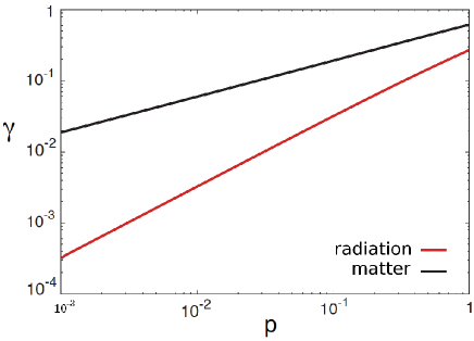
Figure 1: The values of $\gamma$ plotted as a function of $p$ for the radiation and matter-dominated era.

2.2 Loops

In order to maintain the scaling, infinite strings have to continuously release their length in the form of loops. The released length in a Hubble volume per Hubble time is comparable to the length of infinite strings in a Hubble volume. Since the length of a loop formed at time $t$ is given by $\alpha t$, the number density of loops produced between time $t$ and $t+dt$ is

$$\frac{dn}{dt}(t)dt=\frac{dt}{\alpha\gamma^{2}t^{4}}.$$ (5)

The number density of loops is diluted proportional to $a^{-3}$ by cosmic expansion. Therefore, the number density of loops formed between $t_{i}$ and $t_{i}+dt_{i}$ at time $t$ is

$$\frac{dn}{dt_{i}}(t,t_{i})dt_{i}=\frac{dt_{i}}{\alpha\gamma^{2}t_{i}^{4}}\left(\frac{a(t_{i})}{a(t)}\right)^{3}.$$ (6)

After loop formation, it continues to shrink by emitting its energy as GWs. The energy spectrum of GWs from a loop of circumference $l$ per unit time is given by

$$\frac{d\dot{E}}{df}\sim G\mu^{2}l^{-1/3}f^{-4/3}$$ (7)

with a low frequency cutoff at $f\sim l^{-1}$. The total energy emission rate is

$$\dot{E}=\Gamma G\mu^{2},$$ (8)

where $\Gamma$ is set to be $50$ in this paper. Then, the length of a loop formed at $t_{i}$ is

$$l(t,t_{i})=\alpha t_{i}-\Gamma G\mu(t-t_{i}),$$ (9)

at time $t$. Lifetime of a loop formed at $t_{i}$ is given by $\frac{\alpha}{\Gamma G\mu}t_{i}$. If $\alpha<\Gamma G\mu$, they are short-lived, that is, they decay within a Hubble time. If $\alpha>\Gamma G\mu$, loops are long-lived, that is, they live longer than a Hubble time. In this case, loops have a wide range of length from $\alpha t$ to $\Gamma G\mu t$, which corresponds to loops just formed and expiring at some time. The most numerous loops are those of length comparable to $\sim\Gamma G\mu t$.

3 Gravitational waves from cosmic string loops

In this section, we describe the calculation procedure for the burst rate and the spectrum of the GW background, following the formalism in Ref. [11]. Using the result, we show parameter dependence of the burst rate and the background spectrum for several parameter sets.

3.1 Formalism

The linearly polarized waveform of a GW burst emitted in a direction $\mathbf{n}$ by a loop with circumference $l$ at redshift $z$ is expressed as

$$h_{\mu\nu}(t,\mathbf{n})=\int dfh(f,z,l)e^{-2\pi ift}e^{+}_{\mu\nu}(\mathbf{n})\times\Theta(\mathbf{n}\cdot\mathbf{n}_{c}-\cos\theta_{m}(f,z,l))\times\Theta(1-\theta_{m}(f,z,l)),$$ (10)

where $\mathbf{n}_{c}$ is the direction of the center of the burst, which coincides with that of the derivative of the right or left moving mode of the loop, and $\theta_{m}$ is the beaming angle of the GW burst which is given by

$$\theta_{m}(f,z,l)=((1+z)fl)^{-1/3}.$$ (11)

The first Heaviside step function $\Theta$ in Eq. (10) reflects the fact that the burst is emitted into a limited angle, and the second one means that it has a low frequency cutoff at $f\lesssim l^{-1}$ when it is emitted. The polarization tensor (for plus polarization) is expressed as $e^{+}_{\mu\nu}=l_{\mu}m_{\nu}-l_{\nu}m_{\mu}$, where $l_{\mu}=(0,\mathbf{l}),m_{\mu}=(0,\mathbf{m})$ and $\mathbf{l}$ and $\mathbf{m}$ are unit vectors orthogonal to $\mathbf{n}$ and each other.

A GW burst from a loop is most efficiently generated at frequency comparable to $l^{-1}$ and the amplitude of higher frequency modes decrease in proportion to $f^{-4/3}$ . The Fourier transform of the GW amplitude is given by

$$h(f,z,l)\sim\frac{4\pi(12)^{4/3}}{(2\pi)^{1/3}(3\Gamma(1/3))^{2}}\frac{G\mu l}{((1+z)fl)^{1/3}r(z)f}\simeq 2.68\frac{G\mu l}{((1+z)fl)^{1/3}r(z)f},$$ (12)

where

$$r(z)=\int^{z}_{0}dz^{\prime}\frac{1}{H(z^{\prime})},$$ (13)

and $H(z)=H_{0}\left(\Omega_{\Lambda}+\Omega_{m}(1+z)^{3}+\Omega_{r}(1+z)^{4}\right)^{1/2}$ is the Hubble parameter at redshift $z$, where $H_{0}$ is the Hubble parameter of today and $\Omega_{\Lambda}$, $\Omega_{m}$, and $\Omega_{r}$ are the present values of the ratio of the energy density to the total energy density for dark energy, matter and radiation, respectively. Note that one can confirm that this frequency leads to the energy spectrum of GWs from a loop given in Eq. (7) (see, for example, Ref. [45]).

The number of GWs coming to the Earth per unit time, emitted at redshift between $z$ and $z+dz$ by loops formed between $t_{i}$ and $t_{i}+dt_{i}$ is

$$\frac{dR}{dzdt_{i}}dzdt_{i}=\frac{1}{4}\theta_{m}(f,z,l)^{2}\frac{2c}{(1+z)l(t(z),t_{i})}\frac{dn}{dt_{i}}(t(z),t_{i})dt_{i}\frac{dV}{dz}dz\times\Theta(1-\theta_{m}(f,z,l)).$$ (14)

Here, $\frac{1}{4}\theta_{m}(f,z,l)^{2}$ is the factor which represents the fraction of GW bursts beamed towards the Earth. Cusp formation is expected to occur $\mathcal{O}(1)$ times in an oscillation period, which is characterized by parameter $c$. We set it to be $1$ in this paper. The factor $\frac{dV}{dz}dz$ is the volume between $z$ and $z+dz$ at time $t(z)$ and given by

$$\frac{dV}{dz}(z)=\frac{4\pi a^{2}(z)r^{2}(z)}{H(z)(1+z)}.$$ (15)

Since the observables are the amplitude and the frequency of GW bursts, we need a prediction of the burst rate expressed in terms of the given amplitude and frequency. Using Eqs. (9) and (12), we can rewrite Eq. (14) to express the number of GWs coming per unit time which were emitted at redshift $z$ and which have frequency $f$ and amplitude $h$ at the present time

$$\frac{dR}{dzdh}(f,h,z)=\frac{3}{4}\theta^{2}_{m}(f,z,l)\frac{c}{(1+z)h}\frac{1}{\gamma^{2}\alpha t^{4}_{i}}\frac{1}{\alpha+\Gamma G\mu}\left(\frac{a(t_{i})}{a(t)}\right)^{3}\frac{dV}{dz}\Theta(1-\theta_{m}(f,z,l)),$$ (16)

where $l$ and $t_{i}$ can be given as functions of $h$, $z$, and $f$,

$$l(f,h,z)=\left(\frac{hr(z)}{2.68G\mu}(1+z)^{1/3}f^{4/3}\right)^{3/2},$$ (17)

$$t_{i}(f,h,z)=\frac{l(f,h,z)+\Gamma G\mu t(z)}{\alpha+\Gamma G\mu}.$$ (18)

By integrating Eq. (16) in terms of $z$, we get the rate of GWs for the given frequency and amplitude,

$$\frac{dR}{dh}=\int^{\infty}_{0}dz\frac{dR}{dhdz}.$$ (19)

Bursts overlapping each other form a stochastic background. We adopt the criterion in Ref. [13], which counts bursts coming to the Earth with a time interval shorter than the oscillation period of themselves as a component of the GW background. Such bursts have amplitude smaller than $h_{*}$, which is determined for a given frequency as

$$\int^{\infty}_{h_{*}}dh\frac{dR}{dh}=\int^{\infty}_{h_{*}}dh\int^{\infty}_{0}dz\frac{dR}{dzdh}=f.$$ (20)

The amplitude of a stochastic GW background is commonly expressed by $\Omega_{\rm GW}(f)\equiv(d\rho_{\rm GW}/d\ln f)/\rho_{cr}$ where $\rho_{\rm GW}$ is the energy density of the GWs and $\rho_{cr}$ is the critical density of the Universe. Then the spectral amplitude of the GW background is given by summing up all contributions from small bursts,

$$\Omega_{\rm GW}(f)=\frac{2\pi^{2}}{3H_{0}^{2}}f^{3}\int^{h_{*}}_{0}dhh^{2}\frac{dR}{dh}.$$ (21)

3.2 Parameter dependence of the burst rate and the GW background spectrum

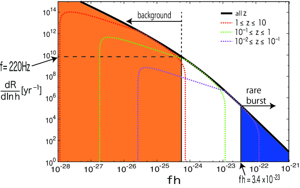
Figure 2: The rate of GW burst $dR/d{\ln}h$ as a function of $fh$, for $G\mu=10^{-7}$, $\alpha=10^{-16}$, $p=1$, and $f=220{\rm Hz}$, represented by the black thick line. Bursts in the left region (orange) form the GW background and those in the right region (blue) are observed as an isolated burst. The red, green and purple dotted line represent the contribution from $1\leq z\leq 10$, $0.1\leq z\leq 1$, and $10^{-2}\leq z\leq 0.1$, respectively.

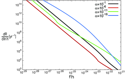
(a) For $G\mu=10^{-7}$, $p=1$, $f=220{\rm Hz}$, and various $\alpha$.

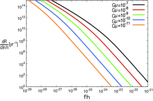
(b) For $\alpha=10^{-16}$, $p=1$, $f=220{\rm Hz}$, and various $G\mu$.

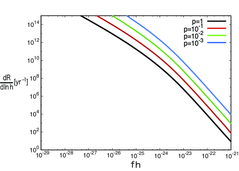
(c) For $G\mu=10^{-7}$, $\alpha=10^{-16}$, $f=220{\rm Hz}$, and various $p$.

Figure 3: The burst rate $dR/d\ln h$ in terms of $fh$ for various parameter sets.

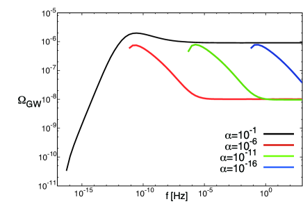
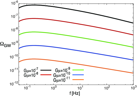
(a) For $G\mu=10^{-7}$, $p=1$, and various $\alpha$. (b) For $\alpha=10^{-16}$, $p=1$, and various $G\mu$.

Figure 4: The background spectrum $\Omega_{\rm GW}$ versus present frequency $f$ for various parameter sets.

Here, we show how the burst rate $dR/dh$ as a function of amplitude $h$ depends on parameters $G\mu$, $\alpha$, and $p$. In Fig. 2, we plot $dR/d{\ln}h$ versus $h$ for $G\mu=10^{-7}$, $\alpha=10^{-16}$, $p=1$, which is evaluated at $f=220{\rm Hz}$, the best-sensitivity frequency of Advanced LIGO.

We set cosmological parameters, to be the WMAP 7-year mean values [51]: the dark energy density divided by the critical density $\Omega_{\Lambda}=0.728$, the dark matter density divided by the critical density $\Omega_{m}=0.272$, the current CMB temperature $T_{0}=2.725{\rm K}$, and the Hubble constant $H_{0}=70.4{\rm km}/{\rm s}/{\rm Mpc}$. We see the natural tendency that stronger bursts have a lower rate. In this figure, we also show the ranges of $h$ which correspond to bursts observed as rare bursts or the GW background by Advanced LIGO. GW bursts whose amplitude are larger than the detector sensitivity, which corresponds to $fh=3.4\times 10^{-23}$ at $f=220{\rm Hz}$ for Advanced LIGO, are observed as rare bursts. In contrast, GW bursts whose rate is larger than their frequency, $f\sim 220{\rm Hz}$ at Advanced LIGO, are measured as the GW background.

GW bursts in each amplitude bin consist of bursts from different redshifts. In order to illustrate which redshift mainly contributes to bursts at a given amplitude, we also plot the contributions to $dR/d\ln h$ from different redshift ranges in Fig. 2. The red, green, and purple dotted line correspond to bursts from $1\leq z\leq 10$, $10^{-1}\leq z\leq 1$, and $10^{-2}\leq z\leq 10^{-1}$, respectively. This indicates that, in this parameter set, bursts detectable by Advanced LIGO come from redshift lower than $z\sim 10^{-2}$, and the GW background consists of bursts emitted at redshifts higher than $z\sim 1$.

Figures 3(a), 3(b), and 3(c) show dependencies of the burst rate on parameters, $G\mu$, $\alpha$, and $p$, respectively. The parametric dependence of the burst rate is the key in studying constraints on cosmic string parameters by GW direct detection experiments, since it determines the direction of the parameter degeneracy, The details are investigated in Appendix A. Here we only give some short explanations. The dependence on $p$ is simplest because a small value of $p$ simply enhances the rate through the factor $\gamma^{-2}$ in Eq. (16). A large value of $G\mu$ basically leads to a larger burst rate because of the enhancement of the amplitude of each burst. However the actual dependence is more nontrivial since the variation of $G\mu$ also changes the typical lifetime of loops, which leads to difference in their density. Variation of $\alpha$ also affects the lifetime of loops, as well as the initial number of loops. Therefore the dependence on $\alpha$ is also not easy to simplify.

We also show the spectrum of the GW background, $\Omega_{\rm GW}$, for different parameter sets in Fig. 4(a) and Fig. 4(b). We also explain details of the parameter dependence of $\Omega_{\rm GW}$ in Appendix B. Physically, $\Omega_{\rm GW}$ at each frequency reflects the energy ratio of expiring loops to the total energy of the Universe at the redshift corresponding to $\min\{\alpha,\Gamma G\mu\}\times t\sim f^{-1}(1+z)^{-1}$ for the radiation-dominated universe, or, for low frequency modes, it reflects the energy of GWs emitted recently.

For these reasons, rare bursts and the background spectrum carry information of cosmic strings at different redshifts, and have different dependence on cosmic string parameters. This is one of the reason they provide different directions of parameter degeneracy in parameter constraints by burst detection and the GW background measurements, as we shall present in the next section.

4 Constraints on cosmic string parameters from future GW experiments

In this section, we investigate how accurately the cosmic string parameters can be determined if GWs from cosmic strings are detected by future experiments. We consider the case where both the GW bursts and the GW background are detected and show their constraints complement each other. Before that, we compute the sensitivities of GW detectors and show the accessible parameter space by current and future experiments.

4.1 Sensitivity for GW detection

In this paper, we assume the worldwide GW network, consists of Advanced LIGO pairs, KAGRA, VIRGO. Additional detectors improve angular resolution and enable precise determination of intrinsic amplitude and polarization of the incoming GWs. Also, since these worldwide GW detectors are directed to different regions of the sky, they provide almost all sky coverage and increase the number of detection events, while each GW detector has limited sky coverage. The detector network also improves sensitivity of the GW background search with the cross-correlation analysis.

4.1.1 Burst

As shown in Eq. (12), the burst signal from a cosmic string cusp would be linearly polarized and have the frequency dependence of $f^{-4/3}$ with cutoffs at low and high frequencies. We assume that the spectrum has the form of

$$h^{+}(f)=Af^{-4/3}\Theta(f_{h}-f)\Theta(f-f_{l}),$$ (22)

where the amplitude $A$ can be read from Eq. (12). The low frequency cutoff corresponds to the size of the loop, whose scale is typically cosmological. So, usually, the cutoff frequency is much lower than the lower frequency limit of direct detection experiments. The high frequency cutoff depends on the viewing angle as $f_{h}\sim 2/(\theta_{\rm obs}^{3}L)$, where $\theta_{\rm obs}$ is defined as the angular separation between the observer’s line of sight and the beam direction of the GW emission.

The total output of the detector is written as a combination of GW signal $h(t)=F^{+}h^{+}(t)$ and detector noise $n(t)$, $s(t)=h(t)+n(t)$, where $F^{+}$ describes the detector response to plus polarized GWs. This function depends on the sky location of the GW source, the polarization angle and the configuration of the detectors, and can be interpreted as the sky area covered by the experiments. For a single detector, one may use the all sky-averaged value for orthogonal arm detectors, $\overline{F^{+}}\sim 1/\sqrt{5}$. For next generation detector network (Advanced LIGO, KAGRA and VIRGO), we assume that the GW detector network has $100\%$ visibility over the whole sky so that $\overline{F^{+}}\sim 1$.

The search for GW bursts signals from cosmic strings is usually performed via matched filtering [52, 20]. The template for cosmic string bursts is usually taken as

$$\tau(f)=f^{-4/3}\Theta(f_{h}-f)(f-f_{l}).$$ (23)

The template is normalized by dividing by $\sigma=\sqrt{(\tau|\tau)}$, where the inner product is defined as

$$(x|y)\equiv 4\Re\int^{\infty}_{0}df\frac{x(f)y^{*}(f)}{S_{n}(f)}.$$ (24)

Thus the normalized template is $\hat{\tau}\equiv\tau/\sigma$, which satisfies $(\hat{\tau}|\hat{\tau})=1$. The noise spectral density $S_{n}(f)$ is defined by $\langle n(f)^{*}n(f)\rangle\equiv S_{n}(f)\delta(f-f^{\prime})/2$, where $\langle\cdots\rangle$ denotes the ensemble average. The noise spectral density for Advanced LIGO is given by [53]

$$S_{n}(f)=10^{-49}\left[x^{-4.14}-\frac{5}{x^{2}}+111\left(\frac{2-2x^{2}+x^{4}}{2+x^{2}}\right)\right]{\rm Hz}^{-1},$$ (25)

where $x=f/(215{\rm Hz})$, and the noise for current LIGO is given by [52].

$$S_{n}(f)=1.09\times 10^{-41}\left(\frac{30{\rm Hz}}{f}\right)^{28}+1.44\times 10^{-45}\left(\frac{100{\rm Hz}}{f}\right)^{4}$$

$$+1.28\times 10^{-46}\left(1+\left(\frac{90{\rm Hz}}{f}\right)^{-2}\right){\rm Hz}^{-1}.$$ (26)

For other GW network observatories, we assume all detectors have the same sensitivity as Advanced LIGO.

The signal to noise ratio $\rho$ is given by the product of the signal and the normalized template as $\rho\equiv(s|\hat{\tau})$. This is equivalent to calculate

$$\rho=\left[4\int^{f_{h}}_{f_{l}}df\frac{|h(f)|^{2}}{S_{n}(f)}\right]^{1/2}.$$ (27)

The low frequency cutoff is determined by the detector’s limitation, which is taken to be $f_{l}=10$Hz for Advanced LIGO and $f_{l}=40$Hz for current LIGO. The high frequency cutoff is different for each burst, depending on the viewing angle. However, in most cases of detection, it is distributed around the most sensitive frequency of the detector [56]. Here, we take $f_{h}=220$Hz for Advanced LIGO and $f_{h}=150$Hz for current LIGO. Taking the detection threshold as $\rho>4$ [10], we find the future GW detector network (Advanced LIGO sensitivity with full sky coverage $\overline{F^{+}}\sim 1$) can detect GW bursts whose amplitudes are larger than $A\simeq 2.1\times 10^{-22}$ ${\rm s}^{-1/3}$, which corresponds to $fh\simeq 3.4\times 10^{-23}$ at $f=220$Hz. For current LIGO (LIGO sensitivity with $\overline{F^{+}}\sim 1/\sqrt{5}$), the detection limit is $A\simeq 9.1\times 10^{-21}$ ${\rm s}^{-1/3}$ which corresponds to $fh\simeq 1.7\times 10^{-21}$ at $f=150$Hz.

4.1.2 Stochastic GW background

The GW background is searched by correlating output signals of two or multiple detectors. One may define the cross correlation signal between two detectors labeled by $I$ and $J$ as [54]

$$S=\int^{T/2}_{-T/2}dt\int^{T/2}_{-T/2}dt^{\prime}s_{I}(t)s_{J}(t^{\prime})Q(t,t^{\prime}),$$ (28)

where $T$ is the observation time and $Q(t,t^{\prime})$ is a filter function. Using the fact that noises of different detectors have no correlation each other, $\langle s_{I}(t)s_{J}(t^{\prime})\rangle\simeq\langle h_{I}(t)h_{J}(t^{\prime})\rangle$, and transforming to Fourier space, the mean value of the signal can be expressed as

$$\mu\equiv\langle S\rangle=\int^{\infty}_{-\infty}df\int^{\infty}_{-\infty}df^{\prime}\delta_{T}(f-f^{\prime})\langle\tilde{h}^{*}_{I}(f)\tilde{h}_{J}(f^{\prime})\rangle\tilde{Q}(f^{\prime}),$$ (29)

where the tilde denotes Fourier-transformed quantities and $\delta_{T}(f-f^{\prime})\equiv\int^{T/2}_{-T/2}dte^{-2\pi ift}=\sin(\pi fT)/\pi f$. The response of the detector is given using $F^{\lambda}$ as

$$\tilde{h}_{I}(f)=\sum_{\lambda}\int d\hat{\bf\Omega}\tilde{h}_{\lambda}(f,{\bf\Omega})e^{-2\pi if\hat{\bf\Omega}\cdot{\bf x}_{I}}F^{\lambda}_{I}(f,{\bf\Omega}),$$ (30)

where $\lambda$ runs for both plus ($+$) and cross ($\times$) polarization and ${\bf x}_{I}$ denotes the position of the detector. Using the relation between the Fourier amplitudes $h_{\lambda}(f,{\bf\Omega})$ and $\Omega_{\rm GW}$,

$$\langle\tilde{h}^{*}_{\lambda}(f,{\bf\Omega})\tilde{h}_{\lambda^{\prime}}(f^{\prime},{\bf\Omega^{\prime}})\rangle=\frac{3H_{0}^{2}}{32\pi^{3}}\delta^{2}({\bf\Omega,\Omega^{\prime}})\frac{1}{2}\delta_{\lambda\lambda^{\prime}}\delta(f-f^{\prime})|f|^{-3}\Omega_{\rm GW}(|f|),$$ (31)

the cross correlation signal is given by

$$\mu=\frac{3H_{0}^{2}}{20\pi^{2}}T\int^{\infty}_{-\infty}df|f|^{-3}\gamma_{IJ}(f)\Omega_{\rm GW}(f)\tilde{Q}(f),$$ (32)

where we define the overlap reduction function as

$$\gamma_{IJ}(f)\equiv\frac{5}{8\pi}\int d\hat{\bf\Omega}(F^{+}_{I}F^{+}_{J}+F^{\times}_{I}F^{\times}_{J})e^{-2\pi if\hat{\bf\Omega}\cdot({\bf x}_{I}-{\bf x}_{J})}.$$ (33)

We calculate the overlap reduction function following the procedure given in Ref. [55], whose Table 2 or Table 3 provides the relative positions of future ground-based GW detectors. In the weak-signal assumption, the variance of the correlation signal is

$$\sigma^{2} \equiv \langle S^{2}\rangle-\langle S\rangle^{2}\approx\langle S^{2}\rangle$$ (34)

$$= \int^{T/2}_{-T/2}dt\int^{T/2}_{-T/2}dt^{\prime}\langle s_{I}(t)s_{J}(t)s_{I}(t^{\prime})s_{J}(t^{\prime})\rangle Q(t)Q(t^{\prime}),$$ (35)

Using $\langle s_{I}(t)s_{J}(t)s_{I}(t^{\prime})s_{J}(t^{\prime})\rangle\simeq\langle n_{I}(t)n_{I}(t^{\prime})\rangle\langle n_{J}(t)n_{J}(t^{\prime})\rangle$ and transforming to Fourier space, this can be expressed in terms of the noise spectral density $S_{n}(f)$ as

$$\sigma^{2}\approx\frac{T}{4}\int^{\infty}_{-\infty}dfS_{n,I}(|f|)S_{n,J}(|f|)|\tilde{Q}(f)|^{2}.$$ (36)

The signal to noise ratio is defined by $\rho\equiv\mu/\sigma$. Choosing the optimal function to maximize the signal to noise ratio, which is $\tilde{Q}(f)\propto\frac{\gamma_{IJ}(|f|)\Omega_{\rm GW}(|f|)}{|f|^{3}S_{n,I}(|f|)S_{n,J}(|f|)}$, we obtain

$$\rho_{IJ}=\frac{3H_{0}^{2}}{10\pi^{2}}\sqrt{2T}\left[\int^{\infty}_{0}df\frac{|\gamma_{IJ}(f)|^{2}\Omega_{\rm GW}(f)^{2}}{f^{6}S_{n,I}(f)S_{n,J}(f)}\right]^{1/2}.$$ (37)

For a network of $N$ detectors, we can make $N(N-1)/2$ independent correlation signals. One can calculate signal to noise ratio as (see Sec. V-C of Ref. [54])

$$\rho=\left[\sum^{N}_{I=1}\sum^{N}_{J<I}\rho_{IJ}^{2}\right]^{1/2}.$$ (38)

Advanced LIGO detector pair would be able to detect the GW background with $\rho>4$ if $\Omega_{\rm GW}>5.1\times 10^{-9}$ (for a flat spectrum) with 3-year observation. The multiple detector network would reach $\Omega_{\rm GW}\sim 3.6\times 10^{-9}$, where we take the range of integration from $10$ to $3000$Hz. The cross-correlation analysis with 2-year run of the current LIGO detector pair has placed an upper limit $\Omega_{\rm GW}<7.2\times 10^{-6}$ [21], which was performed for the frequency band $41.5$-$169.25{\rm Hz}$.

4.2 Accessible parameter space of cosmic string search

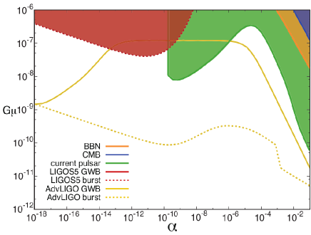
(a) $p=1$

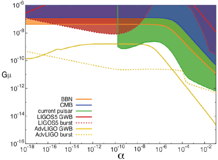
(b) $p=10^{-1}$

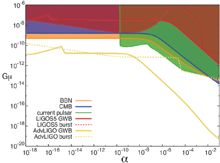
(c) $p=10^{-2}$

Figure 5: The parameter regions excluded by current experiments and cosmological constraints, as well as regions which can be probed by Advanced LIGO, for different values of $p$. The colored regions are excluded by current experiments. Advanced LIGO can probe the region above the yellow solid line with GW background search and that above the yellow dotted line with burst search.

Here, we find the parameter space excluded by current GW experiments and cosmological constraints, and that accessible by future GW experiments. In Fig 5(a), 5(b), and 5(c), we show the parameter regions which are excluded or can be probed by GW experiments in the $\alpha-G\mu$ plane for $p=1$, $10^{-1}$, and $10^{-2}$, respectively. Current constraints are provided by pulsar timing and current LIGO experiments. We also show the cosmological constraints from CMB and BBN, which comes from the fact that the energy density of the GW background, which has the same effect as extra neutrino species on CMB and BBN, must be small at the last scattering epoch and BBN, so as not to distort the fluctuation of CMB and change abundance of various nuclei. For interferometers, we show both parameter regions accessible by burst and GW background search with GW detector network consists of Advanced LIGO and other next generation detectors. For burst detection, we define the detection criterion to be whether the bursts whose amplitude is equal to the detector’s best sensitivity come with a rate higher than $1{\rm yr}^{-1}$. Following the discussion in the previous section, we take the best sensitivity of current LIGO as $fh=1.7\times 10^{-21}$ at $f=150{\rm Hz}$, and the best sensitivity of Advanced LIGO with GW detector network as $fh=3.4\times 10^{-23}$ at $f=220{\rm Hz}$. For the GW background search, we assume it is detectable if the amplitude is higher than $\Omega_{\rm GW}=7.2\times 10^{-6}$ for LIGO, and $\Omega_{\rm GW}=3.6\times 10^{-9}$ for Advanced LIGO.

For the upper limit of $\Omega_{\rm GW}$ from current pulsar timing experiments, we take $1.9\times 10^{-8}$ at $f=3.2\times 10^{-8}{\rm Hz}$ [57]. The CMB provides the constraint that $\int\Omega_{\rm GW}(f)d(\ln f)$ must be less than $1.4\times 10^{-5}$ at the last scattering [58]. The BBN constraint is $\int\Omega_{\rm GW}(f)d(\ln f)<1.6\times 10^{-5}$ at the epoch of BBN [13, 59]. The lower limit of the integral is determined by the lowest frequency of the GWs emitted by largest and youngest loops at the time of CMB and BBN. The upper limit is the frequency of GWs emitted by the earliest loops when they appeared. We consider that the earliest loops are formed at the end of the friction domination, when the temperature of the Universe is $\sim\sqrt{G}\mu$.

The reason why the current pulsar timing experiments constrain only the large $\alpha$ region is that, for a small value of $\alpha$, loops cannot generate GWs at such low frequencies accessible by pulsar timing experiments, which is comparable to $1{\rm yr}^{-1}$. We see that although current constraints on the parameter region are rather severe especially when we consider large $\alpha$, there are still allowed regions which can be probed by Advanced LIGO with both burst detection and the GW background. Choosing parameter values from such a region, we calculate the Fisher information matrix to study how the cosmic string parameters can be constrained by future GW experiments in the following sections.

4.3 Formalism of Fisher analysis

The maximum likelihood method is widely used to estimate model parameters in the analysis of cosmological observations [60]. For a given data set, the set of parameters that is most likely to result in the model prediction are those which maximize likelihood function ${\cal L}$. The error in this estimation can be predicted by calculating the Fisher information matrix, which is defined as

$${\cal F}_{lm}\equiv-\frac{\partial^{2}\ln{\cal L}}{\partial\theta_{l}\partial\theta_{m}}.$$ (39)

Assuming a Gaussian likelihood, the expected error in the parameter $\theta_{l}$ is given by

$$\sigma_{\theta_{l}}=\sqrt{({\cal F}^{-1})_{ll}}$$ (40)

Here, we apply this Fisher matrix formalism to predict how accurately cosmic string parameters can be constrained in future direct detection experiments, for both cases of burst and stochastic background detection.

4.3.1 Burst detection with a single detector

If GW bursts from cosmic strings are detected frequently by GW detectors, we would be able to make a catalogue of the bursts from cosmic strings. Let us suppose that we have a large enough number of samples and the number of observed GW bursts per strain interval $h_{i}$ to $h_{i}+dh_{i}$ is given by

$$N_{i}=\Phi(h_{i})dh_{i},$$ (41)

where $\Phi(h)\equiv dR/dh\times T$ is predictable from the cosmic string parameters as presented in Sec 3. Depending on the detector sensitivity, the catalogue has a magnitude limit of $h=h_{\min}$.

Assuming that the number of GW bursts follows a Poisson distribution [52, 61, 62, 63], the probability of observing $k_{i}$ events in each strain bin is given by

$$p_{i}=\frac{(N_{i})^{k_{i}}e^{-N_{i}}}{k_{i}!}.$$ (42)

Here, $N_{i}$ is a function of $\theta_{l}$, which can be predicted for given parameters as given in Eq. (41). The likelihood function is defined by the total probability of all bins as

$${\cal L}=\prod_{i}\frac{(N_{i})^{k_{i}}e^{-N_{i}}}{k_{i}!}.$$ (43)

Substituting the likelihood into Eq. (39), we obtain the Fisher matrix

$${\cal F}_{lm} = -\frac{\partial^{2}}{\partial\theta_{l}\partial\theta_{m}}\left[\sum_{i}(k_{i}\ln N_{i}+N_{i}-\ln k_{i}!)\right]$$ (44)

$$= -\sum_{i}\left[k_{i}\left(-\frac{\partial N_{i}}{\partial\theta_{l}}\frac{\partial N_{i}}{\partial\theta_{m}}\frac{1}{N_{i}^{2}}+\frac{\partial^{2}N_{i}}{\partial\theta_{l}\partial\theta_{m}}\frac{1}{N_{i}}\right)+\frac{\partial^{2}N_{i}}{\partial\theta_{l}\partial\theta_{m}}\right]$$ (45)

$$= \sum_{i}\frac{\partial N_{i}}{\partial\theta_{l}}\frac{\partial N_{i}}{\partial\theta_{m}}\frac{1}{N_{i}}.$$ (46)

In the last step, we have used $k_{i}\rightarrow N_{i}$ when averaged over large samples. Substituting Eq. (41) and rewriting in terms of integral, the Fisher matrix is given by

$${\cal F}_{lm}=\int^{\infty}_{h_{\rm min}}\frac{\partial\Phi}{\partial\theta_{l}}\frac{\partial\Phi}{\partial\theta_{m}}\frac{1}{\Phi}dh.$$ (47)

We use bursts detectable by the future GW detector network with $\rho>4$, which corresponds to the limit of the catalogue being $fh_{\rm min}\sim 3.4\times 10^{-23}$ at $f=220{\rm Hz}$, as mentioned in Sec. 4.1.1.

4.3.2 Search for the stochastic GW background

The analysis of cross correlation is performed in the frequency domain [64, 65]. Let us consider frequency bins, each of which has a center frequency $f_{i}$ and the width $\delta f_{i}$. We assume the width is much larger than frequency resolution $\delta f_{i}/\Delta f\gg 1$, where $\Delta f\equiv T^{-1}$, so that each bin is statistically independent. Describing Eqs. (32) and (36) in terms of the discrete Fourier transform, the cross-correlated signal and its variance are rewritten as

$$\langle\mu\rangle=2\sum_{i}\frac{3H_{0}^{2}}{20\pi^{2}}\frac{\delta f_{i}}{\Delta f}f_{i}^{-3}\gamma_{IJ}(f_{i})\Omega_{\rm GW}(f_{i})\tilde{Q}(f_{i})\equiv\sum_{i}\langle\mu_{i}\rangle,$$ (48)

$$\sigma^{2}=2\sum_{i}\frac{1}{4}\frac{\delta f_{i}}{\Delta f}S_{n,I}(f_{i})S_{n,J}(f_{i})|\tilde{Q}(f_{i})|^{2}\equiv\sum_{i}\sigma_{i}^{2}.$$ (49)

Assuming Gaussian distribution of the data $\hat{\mu}_{i}$ around the mean value $\langle\mu_{i}\rangle$ with the variance $\sigma_{i}$ in each segment, the probability distribution function is given by

$$p_{i}=\frac{1}{\sqrt{2\pi\sigma_{i}^{2}}}\exp\left[-\frac{(\hat{\mu}_{i}-\langle\mu_{i}\rangle)^{2}}{2\sigma_{i}^{2}}\right].$$ (50)

Then, the likelihood function is defined by the total probability for the whole sample as

$${\cal L}=\prod_{i}\frac{1}{\sqrt{2\pi\sigma_{i}^{2}}}\exp\left[-\frac{(\hat{\mu}_{i}-\langle\mu_{i}\rangle)^{2}}{2\sigma_{i}^{2}}\right].$$ (51)

Substituting the likelihood into Eq. (39), we obtain the Fisher matrix

$${\cal F}_{lm} = -\frac{\partial^{2}}{\partial\theta_{l}\partial\theta_{m}}\sum_{i}\left[-\frac{(\hat{\mu}_{i}-\langle\mu_{i}\rangle)^{2}}{2\sigma_{i}^{2}}\right]$$ (52)

$$= -\sum_{i}\frac{1}{\sigma_{i}^{2}}\left[-\frac{\partial\langle\mu_{i}\rangle}{\partial\theta_{l}}\frac{\partial\langle\mu_{i}\rangle}{\partial\theta_{m}}+(\hat{\mu}_{i}-\langle\mu_{i}\rangle)\frac{\partial^{2}\langle\mu_{i}\rangle}{\partial\theta_{l}\partial\theta_{m}}\right]$$

$$= \sum_{i}\frac{1}{\sigma_{i}^{2}}\frac{\partial\langle\mu_{i}\rangle}{\partial\theta_{l}}\frac{\partial\langle\mu_{i}\rangle}{\partial\theta_{m}}.$$

where the second term of the second line vanishes because $(\hat{\mu_{i}}-\langle\mu_{i}\rangle)$ is zero when averaged over. Substituting $\langle\mu_{i}\rangle$ and $\sigma_{i}$ defined in Eqs. (48) and (49), the Fisher matrix is given as

$${\cal F}_{lm,IJ}=\left(\frac{3H_{0}^{2}}{10\pi^{2}}\right)^{2}2T\int^{\infty}_{0}df\frac{|\gamma_{IJ}(f)|^{2}\partial_{\theta_{l}}\Omega_{\rm GW}(f)\partial_{\theta_{m}}\Omega_{\rm GW}(f)}{f^{6}S_{n,I}(f)S_{n,J}(f)},$$ (53)

For multiple detectors, the Fisher matrix can be calculated with

$${\cal F}_{lm}=\left(\frac{3H_{0}^{2}}{10\pi^{2}}\right)^{2}2T\sum^{N}_{I=1}\sum^{N}_{J<I}\int^{\infty}_{0}df\frac{|\gamma_{IJ}(f)|^{2}\partial_{\theta_{l}}\Omega_{\rm GW}(f)\partial_{\theta_{m}}\Omega_{\rm GW}(f)}{f^{6}S_{n,I}(f)S_{n,J}(f)}.$$ (54)

4.4 Constraints on cosmic string parameters

Using the Fisher matrix formalism presented above, we forecast constraints on cosmic string parameters from future direct detection experiments. In Fig. 6, we present an example of the expected future constraints in the case where the parameters are $G\mu=10^{-7}$, $\alpha=10^{-16}$, $p=1$. Each ellipse represents the $2\sigma$ error contours expected from 3 years of observation with future ground-based GW network (Advanced LIGO, KAGRA and VIRGO with the sensitivity given in Eq. (25)). In this setup, $1.94\times 10^{5}$ bursts are detected with $\rho>4$ by multiple detectors in 3-year observation, and the GW background is detected with $\rho\sim 161$ by correlating outputs of all the detectors. We clearly see the constraints from burst detection (black line) are tighten when it is combined with that from the GW background (red line).

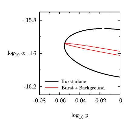
(a) $p-\alpha$

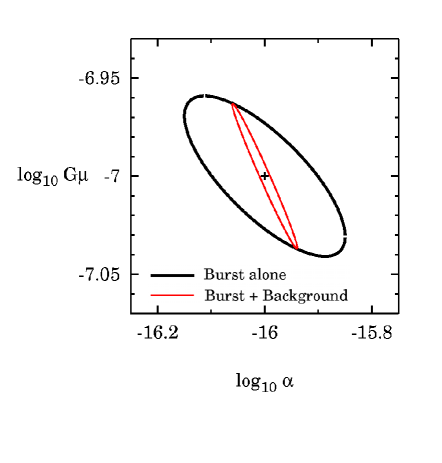
(b) $\alpha-G\mu$

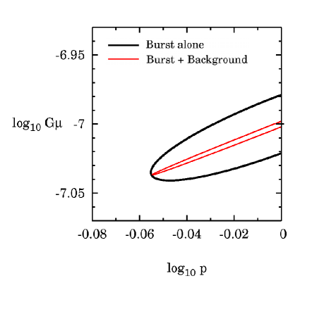
(c) $p-G\mu$

Figure 6: Marginalized $2\sigma$ constraints on cosmic string parameters in $p-\alpha$, $\alpha-G\mu$, and $p-G\mu$ planes, respectively. The fiducial parameters are taken to be $G\mu=10^{-7}$, $\alpha=10^{-16}$, $p=1$. The solid black line represents the constraints from the burst detection alone, and the red line represents the combined constraints from the burst detection and the GW background measurement.

The reason why we can obtain the stronger constraints by combining burst detection and GW background measurements is that the constraints from the two measurements have different parameter degeneracies. In the case of the burst detection, the direction of the parameter degeneracy is determined by the parameter dependence of the rate $dR/d\ln h$, which is presented in Appendix A. The parameter set used here corresponds to the case (iii), i.e. Eq. (58), with $fh_{3,3}\simeq 4.7\times 10^{-25}$. Since GWs larger than $h_{3,3}$ are observed via burst detection, the direction of the parameter degeneracy is $\propto(G\mu)^{2}\alpha^{1/3}p^{-1}$. In the case of the GW background, the direction of the parameter degeneracy is determined by the parameter dependence of $\Omega_{\rm GW}$, which is investigated in Appendix B. In this parameter set (the case (iii)), the GW background is given by (65), and the second term dominates the first term if it is evaluated at the frequency of Advanced LIGO. Thus, the constraints from the GW background has the parameter degeneracy of $\propto G\mu\alpha^{-1/3}p^{-1}$. The constraints from the GW background have strong parameter degeneracies since the observable is basically only $\Omega_{\rm GW}$ at $f=220$Hz. By combining it with the constraints from bursts, the degeneracies are broken.

Here, we would like to mention when these bursts and the background detectable by Advanced LIGO are emitted in the case of the parameter set we take above. As mentioned in Appendix A, bursts of given frequency $f$ and amplitude $h$ are mainly emitted at redshift which satisfies $l(f,h,z)\sim\alpha t(z)$ for $\alpha<\Gamma G\mu$, so bursts detectable by Advanced LIGO are generated at $z\ll 1$. To be more specific, GWs of amplitude equal to the sensitivity of Advanced LIGO, $fh\simeq 3.4\times 10^{-23}$, and of frequency $f=220{\rm Hz}$ come from $z\sim 3.6\times 10^{-2}$, and those detected once per year by Advanced LIGO, which have $fh\sim 10^{-21}$ and $f=220{\rm Hz}$, come from $z\sim 10^{-3}$. The main contribution on the GW background comes from GWs emitted at redshift which satisfies $f(1+z)\sim\alpha t(z)$ in the radiation-dominated epoch and those emitted at $z\sim 1$. At the frequency of Advanced LIGO, the contribution from the latter is larger.

5 Conclusion

Future GW experiments can be a unique and useful tool to test the existence of cosmic strings. If GWs from cosmic strings are detected, they could provide important constraints on cosmic string parameters. In this paper, we have studied the potential of upcoming ground-based GW experiments to search for signals from cosmic strings and estimated the power to place constraints on cosmic string parameters.

The key point of this paper is that GW experiments can search for cosmic string signals both in the way of burst detection and GW background measurements. First, we find the parameter region where GWs from cosmic strings are detectable by future experiments considering the both cases. Furthermore, we investigate constraints on cosmic string parameters obtainable from direct detection measurements of the GW bursts and the GW background, and found that their information is complementary from each other. Thus, if both the GW bursts and the GW background are detected, we can tighten the constraints on cosmic string parameters by combining data from the two different measurements. Although we demonstrate only the case of ground-based experiments, this is also the case in future satellite experiments like BBO and DECIGO which is designed to search for both GW bursts and GW backgrounds.

One thing we must note is that there would be other sources of GW bursts and GW backgrounds. There are surely many astrophysical candidates which generate GW bursts. However, since GW bursts from cosmic strings have a characteristic frequency dependence, cosmic string bursts could be distinguished from those from other sources. In the case of the GW background, although there is no certain source, some models can predict a GW background around the frequency band of LIGO sensitivity. We could also use information on the frequency dependence of the spectrum, but it may be difficult to identify whether the detected GW background originates from cosmic strings or other models. However, although it depends on the values of the cosmic string parameters, we may be able to use other observations which explore different frequency ranges of GWs such as CMB $B$-mode measurements [66, 67, 68, 69, 70, 71, 72, 73] and pulsar timing experiments [57, 74] to verify the GW background from cosmic string, which will be studied in our future work.

Appendix

Appendix A Parametric dependence of the burst rate

In this appendix, we roughly estimate the dependence of the burst rate on cosmic string parameters. Cosmic strings expiring at each epoch give dominant contribution to GWs, because they are the most numerous. So, roughly speaking, we only need to estimate their contribution to the burst rate, as shown formally below. Since we are interested in high frequency GWs detectable by ground-based GW experiments, we consider bursts which satisfy $f>\left(\min\{\alpha,\Gamma G\mu\}\right)^{-1}t^{-1}(z_{eq})(1+z_{eq})^{-1}$, which means that expiring loops start to contribute to relevant frequencies in the radiation-dominated era and their contribution continues until today.

The rate $dR/d\ln h$ is derived by integrating Eq. (16) in terms of $z$. Using Eqs. (11), (17), and (18), we find that in the case where $\alpha\gg\Gamma G\mu$, so loops are long-lived, the dominant contribution to the integration of Eq. (16) comes from the redshift around $z_{m}$ which satisfies

$$l(f,h,z_{m})=\Gamma G\mu t(z_{m}),$$ (55)

for large $h$. The size of loops which emit GW bursts of frequency $f$ and amplitude $h$ depends on when they are emitted and it is denoted by $l(f,h,z)$. Equation (55) means that, for a given frequency and amplitude, GWs are mostly generated by loops expiring at redshift $z_{m}$. Therefore, we can roughly estimate the rate by $dR/dh\sim z_{m}(f,h)\times\frac{dR}{dhdz}(f,h,z_{m}(f,h))$, neglecting accuracy of $\mathcal{O}(1)$ numerical factors. Note that for too small $h$, there is no solution which satisfies both Eq. (55) and $f(1+z_{m})>l^{-1}(f,h,z_{m})$, which corresponds to the lower frequency cutoff of bursts. In this case, the main contribution to the $z$ integral of Eq. (16) comes from $z_{m}$ which satisfies $f(1+z_{m})=l^{-1}(f,h,z_{m})$.

In the case of short-lived loops, $\alpha\ll\Gamma G\mu$, $z_{m}$ is given by $l(f,h,z_{m})=\alpha t(z_{m})$. In this case, if we consider small $h$, any value of $z$ does not satisfy $l(f,h,z)=\alpha t(z)$, so $dR/d\ln h$ is strongly suppressed.

The rate of GW burst depends on when bursts are mainly emitted and when loops which emit such bursts are formed. We summarize the results below:

(i) $\alpha>\Gamma G\mu\left(\frac{\Omega_{m}}{\Omega_{r}}\right)^{3/2}$

(Here, $\Omega_{r}$ is the current energy density of radiation divided by the critical density.)

In this case, loops are so long-lived that those formed in the matter-dominated era does not decay before today. In other words, loops which have decayed by today are formed in the radiation-dominated era.

The burst rate is given as follows.

$$\frac{dR}{d\ln h}(f,h)\sim\begin{cases}&(G\mu)^{1/2}\alpha^{1/2}\gamma_{r}^{-2}\left(\frac{\Omega_{m}}{\Omega_{r}}\right)^{-1/4}f^{3/2}t_{0}h^{-1/2}\quad;h<\left(\frac{\Omega_{m}}{\Omega_{r}}\right)^{-1/2}f^{-3}t_{0}^{-2}\equiv h_{1,1}\\ &(G\mu)^{1/2}\alpha^{1/2}\gamma_{r}^{-2}\left(\frac{\Omega_{m}}{\Omega_{r}}\right)^{-11/10}f^{-18/5}t_{0}^{-12/5}h^{-11/5}\\ &\quad;h_{1,1}<h<(G\mu)^{5/3}f^{-4/3}t_{0}^{-1/3}\left(\frac{\Omega_{m}}{\Omega_{r}}\right)^{-4/3}\equiv h_{1,2}\\ &(G\mu)^{1/16}\alpha^{1/2}\gamma_{r}^{-2}\left(\frac{\Omega_{m}}{\Omega_{r}}\right)^{-3/4}f^{-13/4}t_{0}^{-37/16}h^{-31/16}\\ &\quad;h_{1,2}<h<(G\mu)^{5/3}f^{-4/3}t_{0}^{-1/3}\equiv h_{1,3}\\ &(G\mu)^{11/6}\alpha^{1/2}\gamma_{r}^{-2}\left(\frac{\Omega_{m}}{\Omega_{r}}\right)^{-3/4}f^{-14/3}t_{0}^{-8/3}h^{-2}\quad;h>h_{1,3}\end{cases},$$ (56)

where $t_{0}$ is the present age of the Universe.

Bursts whose amplitudes are $h_{1,1}<h<h_{1,2}$, $h_{1,2}<h<h_{1,3}$, and $h>h_{1,3}$ correspond to those emitted in the radiation-dominated era, in the matter-dominated era, and at redshift smaller than $1$, respectively. If $h<h_{1,1}$, any $z_{m}$ does not satisfy $f(1+z_{m})\sim l^{-1}(f,h,z_{m})$. Therefore, bursts which have amplitude of $h<h_{1,1}$ are emitted in the radiation-dominated era not by loops expiring but by loops which still have their lifetime.

Increase of $G\mu$ enhances the amplitude of each burst. Since bursts of a given amplitude can come from earlier epochs and more distant points for larger $G\mu$, their number increases. This is why the rate is proportional to a positive power of $G\mu$. However, there is also an effect which decreases the rate with increasing $G\mu$, that is, reduction of the loop lifetime and the density of expiring loops due to the enhancement of the efficiency of the GW emission. Note that loops formed earlier are more abundant than those formed later despite more dilution by the cosmic expansion, since the density at their formation is larger for older loops. The total power of $G\mu$ is determined by these effects. As $\alpha$ increases, the elongation of loop lifetime enhances the rate but the initial number of loops decreases. In this case, the former is more efficient and the power of $\alpha$ in Eq. (56) becomes positive.

(ii) $\Gamma G\mu<\alpha<\Gamma G\mu\left(\frac{\Omega_{m}}{\Omega_{r}}\right)^{3/2}$

In this case, loops which expire at small redshift are formed in the matter-dominated era. The burst rate is given by

$$\frac{dR}{d\ln h}(f,h)\sim\begin{cases}&(G\mu)^{1/2}\alpha^{1/2}\gamma_{r}^{-2}\left(\frac{\Omega_{m}}{\Omega_{r}}\right)^{-1/4}f^{3/2}t_{0}h^{-1/2}\quad;h<\left(\frac{\Omega_{m}}{\Omega_{r}}\right)^{-1/2}f^{-3}t_{0}^{-2}\equiv h_{2,1}\\ &(G\mu)^{1/2}\alpha^{1/2}\gamma_{r}^{-2}\left(\frac{\Omega_{m}}{\Omega_{r}}\right)^{-11/10}f^{-18/5}t_{0}^{-12/5}h^{-11/5}\\ &\quad;h_{2,1}<h<(G\mu)^{5/3}f^{-4/3}t_{0}^{-1/3}\left(\frac{\Omega_{m}}{\Omega_{r}}\right)^{-4/3}\equiv h_{2,2}\\ &(G\mu)^{1/16}\alpha^{1/2}\gamma_{r}^{-2}\left(\frac{\Omega_{m}}{\Omega_{r}}\right)^{-3/4}f^{-13/4}t_{0}^{-37/16}h^{-31/16}\\ &\quad;h_{2,1}<h<(G\mu)^{7/9}\alpha^{8/9}f^{-4/3}t_{0}^{-1/3}\left(\frac{\Omega_{m}}{\Omega_{r}}\right)^{-4/3}\equiv h_{2,3}\\ &(G\mu)^{-3/8}\gamma_{m}^{-2}f^{-5/2}t_{0}^{-17/8}h^{-11/8}\\ &\quad;h_{2,2}<h<(G\mu)^{5/3}f^{-4/3}t_{0}^{-1/3}\equiv h_{2,4}\\ &(G\mu)^{7/3}\gamma_{m}^{-2}f^{-14/3}t_{0}^{-8/3}h^{-3}\quad;h>h_{2,4}\end{cases}.$$ (57)

Bursts whose amplitudes are $h_{2,1}<h<h_{2,2}$ and $h_{2,2}<h<h_{2,3}$ correspond to those emitted in the radiation-dominated era and in the matter-dominated era by loops formed in the radiation-dominated era. On the other hand, bursts in the range of $h_{2,3}<h<h_{2,4}$ and $h>h_{2,4}$ are emitted at redshift $1<z<z_{eq}$ and $z<1$ by loops formed after the matter-radiation equality. These are mainly emitted by expiring loops. Bursts of $h<h_{2,1}$, on the other hand, are emitted by loops which do not expire soon.

(iii) $\alpha<\Gamma G\mu$

In this case, loops are short-lived. The rate is given by

$$\frac{dR}{d\ln h}(f,h)\sim\begin{cases}&(G\mu)^{6/5}\alpha^{-1/5}\gamma_{r}^{-2}\left(\frac{\Omega_{m}}{\Omega_{r}}\right)^{-11/10}f^{-18/5}t_{0}^{-12/5}h^{-11/5}\\ &\qquad;G\mu\alpha^{-1}f^{-3}t_{0}^{-2}\left(\frac{\Omega_{m}}{\Omega_{r}}\right)^{-1/2}\equiv h_{3,1}<h<G\mu\alpha^{2/3}f^{-4/3}t_{0}^{-1/3}\left(\frac{\Omega_{m}}{\Omega_{r}}\right)^{-4/3}\equiv h_{3,2}\\ &(G\mu)^{3/8}\alpha^{-3/4}\gamma_{m}^{-2}f^{-5/2}t_{0}^{-17/8}h^{-11/8}\\ &\qquad;h_{3,2}<h<G\mu\alpha^{2/3}f^{-4/3}t_{0}^{-1/3}\equiv h_{3,3}\\ &(G\mu)^{2}\alpha^{1/3}\gamma_{m}^{-2}f^{-14/3}t_{0}^{-8/3}h^{-3}\qquad;h>h_{3,3}\end{cases}.$$ (58)

Bursts in the range of $h_{3,1}<h<h_{3,2}$, $h_{3,2}<h<h_{3,3}$, and $h>h_{3,3}$ are emitted in the radiation-dominated era, in the matter-dominated era, and at $z\ll 1$, respectively. The burst rate for $h<h_{3,1}$ is suppressed for the same reason as $h<h_{1,1}$ and $h<h_{2,1}$. In these cases, elongation or shortening of loop lifetime do not affect the rate and the rate depends only on parameters through time of burst emission and initial number of loops.

Appendix B Parametric dependence of the spectrum of the stochastic GW background

In this appendix, we roughly describe the amplitude of $\Omega_{\rm GW}$ in terms of cosmic string parameters. In the same way as the previous section, we consider only high frequency GWs.

(i) $\alpha>\Gamma G\mu\left(\frac{\Omega_{m}}{\Omega_{r}}\right)^{3/2}$

In this cases, we find through Eq. (56) that the dominant contribution to the integral of $h^{2}\frac{dR}{dh}$ in Eq. (21) comes from $h\sim h_{1,1}$ or $h\sim h_{1,3}$. Approximating that the contribution to $\int d\ln hh^{3}\frac{dR}{dh}$ only comes from these GWs simply as $h_{m}^{3}\frac{dR}{dh}(h_{m})$, where $h_{m}$ is $h_{1,1}$ or $h_{1,3}$, we get

$$\Omega_{\rm GW}\sim(G\mu)^{1/2}\alpha^{1/2}\gamma_{r}^{-2}\frac{\Omega_{r}}{\Omega_{m}}+(G\mu)^{1/6}\alpha^{1/2}\gamma_{r}^{-2}\left(\frac{\Omega_{m}}{\Omega_{r}}\right)^{-3/4}t_{0}^{-1/3}f^{-1/3}.$$ (59)

The first term, the contribution from $h\sim h_{1,1}$, represents the GWs emitted when loops decay in the radiation-dominated era, and the second one, the contribution from $h\sim h_{1,3}$, corresponds to GWs emitted at $z\sim 1$ by loops which expired recently or are decaying today.

We can estimate that the first term is equal to the energy of loops expiring at time $t$ (redshift $z$) which satisfies $\Gamma G\mu t\sim 1/f(1+z)$ as

$$\Omega_{\rm GW} \sim\frac{\rho_{loop}(t)|_{l\sim\Gamma G\mu t}}{\rho_{tot}(t)}\frac{\Omega_{r}}{\Omega_{m}}$$

$$\sim\frac{\rho_{loop}(t_{i})|_{l\sim\alpha t_{i}}}{\rho_{tot}(t_{i})}\frac{1+z_{i}}{1+z}\frac{\Omega_{r}}{\Omega_{m}}$$

$$\sim G\mu\gamma_{r}^{-2}\left(\frac{\alpha}{\Gamma G\mu}\right)^{1/2}\frac{\Omega_{r}}{\Omega_{m}}$$

$$\sim(G\mu)^{1/2}\alpha^{1/2}\gamma_{r}^{-2}\frac{\Omega_{r}}{\Omega_{m}}.$$ (60)

Here, $t_{i}$ and $z_{i}$ are the time and redshift of the loop formation respectively, which is related to the time of GW emission as $t_{i}\sim\frac{\Gamma G\mu}{\alpha}t$, and the factor $\frac{\Omega_{r}}{\Omega_{m}}$ denote the dilution of GWs from the matter-radiation equality to now.

The second term can be estimated as follows,

$$\Omega_{\rm GW}\sim\frac{1}{\gamma_{r}^{2}\alpha t_{i}^{3}}(1+z_{i})^{3}\times\frac{d\dot{E}}{df}(f)f\times t_{0}\times\frac{1}{\rho_{cr}}\sim(G\mu)^{1/6}\alpha^{1/2}\gamma_{r}^{-2}\left(\frac{\Omega_{m}}{\Omega_{r}}\right)^{-3/4}t_{0}^{-1/3}f^{-1/3},$$ (61)

where $t_{i}\sim\frac{\Gamma G\mu}{\alpha}t_{0}$ and $z_{i}$ are the time and the redshift when loops expiring today are formed. Note that the number of GWs emitted recently is so small that it might not be regarded as a part of the background. The condition $\frac{dR}{d\ln h}(h=h_{1,3})>f$ leads to

$$(G\mu)^{-19/6}\alpha^{1/2}\gamma_{r}^{-2}\left(\frac{\Omega_{m}}{\Omega_{r}}\right)^{-3/4}(ft_{0})^{-5/3}>1,$$ (62)

which can be satisfied by small $G\mu$, for example $G\mu\lesssim 10^{-11}$, for $f\sim 100{\rm Hz},\alpha=0.1,p=1$.

(ii) $\Gamma G\mu<\alpha<\Gamma G\mu\left(\frac{\Omega_{m}}{\Omega_{r}}\right)^{3/2}$

One can get $\Omega_{\rm GW}$ by estimating $\int dhh^{2}\frac{dR}{dh}$ in the same way as demonstrated above. The result is

$$\Omega_{\rm GW}\sim(G\mu)^{1/2}\alpha^{1/2}\gamma_{r}^{-2}\frac{\Omega_{r}}{\Omega_{m}}+(G\mu)^{2/3}\gamma_{m}^{-2}t_{0}^{-1/3}f^{-1/3}.$$ (63)

Again, the first term corresponds to the GWs emitted by loops decayed in the radiation-dominated era and the second one is the contribution from loops expiring today. The first term is identical to the one in Eq. (59). On the other hand, the second one is different because loops expiring today are formed after matter-radiation equality in this case.

The condition to include the second term in $\Omega_{\rm GW}$ is

$$(G\mu)^{-8/3}\gamma_{m}^{-2}(ft_{0})^{-5/3}>1.$$ (64)

For $f\sim 100{\rm Hz}$ and $p=1$, this reads $G\mu\lesssim 10^{-12}$.

(iii) $\alpha<\Gamma G\mu$

In this case, we get

$$\Omega_{\rm GW}\sim G\mu\gamma_{r}^{-2}\frac{\Omega_{r}}{\Omega_{m}}+G\mu\gamma_{m}^{-2}\alpha^{-1/3}t_{0}^{-1/3}f^{-1/3}.$$ (65)

Again, the first term is the contribution from GWs emitted in the radiation-dominated era and the second one represents GWs emitted recently. The first term coincides with the ratio of the energy of the infinite string network to the total energy, $\sim G\mu\gamma^{-2}$, except the dilution factor $\frac{\Omega_{r}}{\Omega_{m}}$, because, in this case, loops released from infinite strings immediately expire by radiating GWs. The second term also consists of $G\mu\gamma^{-2}$ and the factor $(f\alpha t_{0})^{-1/3}$, which corresponds to the tilt of the spectrum of emitted GWs.

The condition to include the second term in $\Omega_{\rm GW}$ is

$$(G\mu)^{-1}\alpha^{-5/3}\gamma_{m}^{-2}(ft_{0})^{-5/3}>1,$$ (66)

which is relatively easy to satisfy for small $\alpha$. For example, this reads $G\mu\lesssim 10^{-6}$ for $f\sim 100{\rm Hz}$, $\alpha=10^{-16}$ and $p=1$.

References

- [1] T. W. B. Kibble, J. Phys. A 9, 1387 (1976).
- [2] A. Vilenkin and E. P. S. Shellard, “Cosmic Strings and Other Topological Defects,” Cambridge University Press, Cambridge, England (1994).
- [3] S. Sarangi and S. H. H. Tye, Phys. Lett. B 536, 185 (2002) [arXiv:hep-th/0204074].
- [4] N. T. Jones, H. Stoica, S. H. H. Tye, Phys. Lett. B563, 6-14 (2003). [hep-th/0303269].
- [5] G. Dvali and A. Vilenkin, JCAP 0403, 010 (2004) [arXiv:hep-th/0312007].
- [6] A. Vilenkin, Phys. Lett. B107, 47-50 (1981).
- [7] C. J. Hogan, M. J. Rees, Nature 311, 109-113 (1984).
- [8] R. R. Caldwell and B. Allen, Phys. Rev. D 45, 3447 (1992).
- [9] R. R. Caldwell, R. A. Battye and E. P. S. Shellard, Phys. Rev. D 54, 7146 (1996) [arXiv:astro-ph/9607130].
- [10] T. Damour and A. Vilenkin, Phys. Rev. Lett. 85, 3761 (2000) [arXiv:gr-qc/0004075].
- [11] T. Damour and A. Vilenkin, Phys. Rev. D 64, 064008 (2001) [arXiv:gr-qc/0104026].
- [12] T. Damour and A. Vilenkin, Phys. Rev. D 71, 063510 (2005) [arXiv:hep-th/0410222].
- [13] X. Siemens, V. Mandic and J. Creighton, Phys. Rev. Lett. 98, 111101 (2007) [arXiv:astro-ph/0610920].
- [14] M. R. DePies and C. J. Hogan, Phys. Rev. D 75, 125006 (2007) [arXiv:astro-ph/0702335];
- [15] M. Kawasaki, K. Miyamoto, K. Nakayama, Phys. Rev. D81, 103523 (2010). [arXiv:1002.0652 [astro-ph.CO]].
- [16] S. Olmez, V. Mandic, X. Siemens, Phys. Rev. D81, 104028 (2010). [arXiv:1004.0890 [astro-ph.CO]].
- [17] P. Binetruy, A. Bohe, C. Caprini and J. -F. Dufaux, JCAP 1206, 027 (2012). [arXiv:1201.0983 [gr-qc]].
- [18] P. Binetruy, A. Bohe, T. Hertog and D. A. Steer, Phys. Rev. D 82, 126007 (2010) [arXiv:1009.2484 [hep-th]].
- [19] A. Bohe, Phys. Rev. D 84, 065016 (2011) [arXiv:1103.0768 [hep-th]].
- [20] B. P. Abbott et al. [LIGO Scientific Collaboration], Phys. Rev. D 80, 062002 (2009) [arXiv:0904.4718 [astro-ph.CO]].
- [21] B. P. Abbott et al. [ LIGO Scientific and VIRGO Collaborations ], Nature 460, 990 (2009). [arXiv:0910.5772 [astro-ph.CO]].
- [22] D. Sigg [LIGO Scientific Collaboration], Class. Quant. Grav. 25, 114041 (2008).
- [23] K. Kuroda [LCGT Collaboration], Class. Quant. Grav. 27, 084004 (2010).
- [24] T. Accadia et al., Class. Quant. Grav. 28, 114002 (2011).
- [25] D. P. Bennett, F. R. Bouchet, Phys. Rev. Lett. 60, 257 (1988), Phys. Rev. Lett. 63, 2776 (1989), Phys. Rev. D41, 2408 (1990).
- [26] B. Allen, E. P. S. Shellard, Phys. Rev. Lett. 64, 119-122 (1990).
- [27] G. R. Vincent, M. Hindmarsh, M. Sakellariadou, Phys. Rev. D56, 637-646 (1997). [astro-ph/9612135].
- [28] V. Vanchurin, K. D. Olum, A. Vilenkin, Phys. Rev. D74, 063527 (2006). [gr-qc/0511159].
- [29] C. Ringeval, M. Sakellariadou, F. Bouchet, JCAP 0702, 023 (2007). [astro-ph/0511646].
- [30] C. J. A. P. Martins, E. P. S. Shellard, Phys. Rev. D73, 043515 (2006). [astro-ph/0511792].
- [31] K. D. Olum, V. Vanchurin, Phys. Rev. D75, 063521 (2007). [astro-ph/0610419].
- [32] X. Siemens, K. D. Olum, A. Vilenkin, Phys. Rev. D66, 043501 (2002). [gr-qc/0203006].
- [33] J. Polchinski, J. V. Rocha, Phys. Rev. D74, 083504 (2006). [hep-ph/0606205].
- [34] F. Dubath, J. Polchinski, J. V. Rocha, Phys. Rev. D77, 123528 (2008). [arXiv:0711.0994 [astro-ph]].
- [35] V. Vanchurin, Phys. Rev. D77, 063532 (2008). [arXiv:0712.2236 [gr-qc]].
- [36] L. Lorenz, C. Ringeval and M. Sakellariadou, JCAP 1010, 003 (2010) [arXiv:1006.0931 [astro-ph.CO]].
- [37] M. G. Jackson, N. T. Jones, J. Polchinski, JHEP 0510, 013 (2005). [hep-th/0405229].
- [38] A. Hanany, K. Hashimoto, JHEP 0506, 021 (2005). [hep-th/0501031].
- [39] M. G. Jackson, JHEP 0709, 035 (2007). [arXiv:0706.1264 [hep-th]].
- [40] M. Sakellariadou, JCAP 0504, 003 (2005). [hep-th/0410234].
- [41] A. Avgoustidis, E. P. S. Shellard, Phys. Rev. D73, 041301 (2006). [astro-ph/0512582].
- [42] K. Takahashi, A. Naruko, Y. Sendouda, D. Yamauchi, C. -M. Yoo, M. Sasaki, JCAP 0910, 003 (2009). [arXiv:0811.4698 [astro-ph]].
- [43] C. J. A. P. Martins, E. P. S. Shellard, Phys. Rev. D54, 2535-2556 (1996). [arXiv:hep-ph/9602271].
- [44] C. J. A. P. Martins and E. P. S. Shellard, Phys. Rev. D 65, 043514 (2002) [hep-ph/0003298].
- [45] S. Weinberg, “Gravitation and Cosmology,” John Wiley and Sons (1972).
- [46] T. Regimbau, S. Giampanis, X. Siemens and V. Mandic, Phys. Rev. D 85, 066001 (2012) [arXiv:1111.6638 [astro-ph.CO]].
- [47] S. Drasco and E. E. Flanagan, Phys. Rev. D 67, 082003 (2003) [gr-qc/0210032].
- [48] N. Seto, Astrophys. J. 683, L95 (2008) [arXiv:0807.1151 [astro-ph]].
- [49] N. Seto, Phys. Rev. D 80, 043003 (2009) [arXiv:0908.0228 [gr-qc]].
- [50] B. Allen, E. P. S. Shellard, Phys. Rev. D45, 1898-1912 (1992).
- [51] E. Komatsu et al. [ WMAP Collaboration ], Astrophys. J. Suppl. 192, 18 (2011). [arXiv:1001.4538 [astro-ph.CO]].
- [52] X. Siemens, J. Creighton, I. Maor, S. Ray Majumder, K. Cannon and J. Read, Phys. Rev. D 73, 105001 (2006) [arXiv:gr-qc/0603115].
- [53] J. S. Key and N. J. Cornish, Phys. Rev. D 79, 043014 (2009) [arXiv:0812.1590 [gr-qc]].
- [54] B. Allen and J. D. Romano, Phys. Rev. D 59, 102001 (1999) [arXiv:gr-qc/9710117].
- [55] A. Nishizawa, A. Taruya, K. Hayama, S. Kawamura and M. a. Sakagami, Phys. Rev. D 79, 082002 (2009) [arXiv:0903.0528 [astro-ph.CO]].
- [56] M. I. Cohen, C. Cutler and M. Vallisneri, Class. Quant. Grav. 27, 185012 (2010) [arXiv:1002.4153 [gr-qc]].
- [57] F. A. Jenet, G. B. Hobbs, W. van Straten, R. N. Manchester, M. Bailes, J. P. W. Verbiest, R. T. Edwards, A. W. Hotan et al., Astrophys. J. 653, 1571-1576 (2006). [astro-ph/0609013].
- [58] T. L. Smith, E. Pierpaoli, M. Kamionkowski, Phys. Rev. Lett. 97, 021301 (2006). [astro-ph/0603144].
- [59] R. H. Cyburt, B. D. Fields, K. A. Olive, E. Skillman, Astropart. Phys. 23, 313-323 (2005). [astro-ph/0408033].
- [60] M. Tegmark, A. Taylor and A. Heavens, Astrophys. J. 480, 22 (1997) [arXiv:astro-ph/9603021].
- [61] B. Abbott et al. [LIGO Collaboration], Phys. Rev. D 69, 102001 (2004) [gr-qc/0312056].
- [62] L. Baggio et al. [AURIGA and LIGO Scientific Collaborations], Class. Quant. Grav. 25, 095004 (2008) [arXiv:0710.0497 [gr-qc]].
- [63] L. S. Finn and A. N. Lommen, Astrophys. J. 718, 1400 (2010) [arXiv:1004.3499 [astro-ph.IM]].
- [64] B. Abbott et al. [LIGO Scientific Collaboration], Phys. Rev. D 69, 122004 (2004) [gr-qc/0312088].
- [65] N. Seto, Phys. Rev. D 73, 063001 (2006) [arXiv:gr-qc/0510067].
- [66] U. Seljak, U. -L. Pen, N. Turok, Phys. Rev. Lett. 79, 1615-1618 (1997). [astro-ph/9704231].
- [67] K. Benabed, F. Bernardeau, Phys. Rev. D61, 123510 (2000).
- [68] U. Seljak, A. Slosar, Phys. Rev. D74, 063523 (2006). [astro-ph/0604143].
- [69] N. Bevis, M. Hindmarsh, M. Kunz, J. Urrestilla, Phys. Rev. D76, 043005 (2007). [arXiv:0704.3800 [astro-ph]].
- [70] L. Pogosian, M. Wyman, Phys. Rev. D77, 083509 (2008). [arXiv:0711.0747 [astro-ph]].
- [71] M. Kawasaki, K. Miyamoto and K. Nakayama, Phys. Rev. D 82, 103504 (2010) [arXiv:1003.3701 [astro-ph.CO]].
- [72] N. Bevis, M. Hindmarsh, M. Kunz, J. Urrestilla, Phys. Rev. D82, 065004 (2010). [arXiv:1005.2663 [astro-ph.CO]].
- [73] P. Mukherjee, J. Urrestilla, M. Kunz, A. R. Liddle, N. Bevis, M. Hindmarsh, Phys. Rev. D83, 043003 (2011). [arXiv:1010.5662 [astro-ph.CO]].
- [74] M. S. Pshirkov, A. V. Tuntsov, Phys. Rev. D81, 083519 (2010). [arXiv:0911.4955 [astro-ph.CO]].