The critical behaviour of the Ising model on the 4-dimensional lattice

Abstract

In this paper we investigate the nature of the singularity of the Ising model of the 4-dimensional cubic lattice. It is rigorously known that the specific heat has critical exponent $\alpha=0$ but a non-rigorous field-theory argument predicts an unbounded specific heat with a logarithmic singularity at $T_{c}$.

We find that within the given accuracy the canonical ensemble data is consistent both with a logarithmic singularity and a bounded specific heat, but that the micro-canonical ensemble lends stronger support to a bounded specific heat.

Our conclusion is that either much larger system sizes are needed for Monte Carlo studies of this model in four dimensions or the field theory prediction of a logarithmic singularity is wrong.

I Introduction

In dimension $D\geq 5$ it is known from Aizenman (1981, 1982) that the Ising model on the cubic lattice exhibits mean-field critical exponents at the critical temperature. Even earlier it was shown Sokal (1979) that the specific heat obeys the mean-field exponent $\alpha=0$ for $D\geq 4$, and that for $D\geq 5$ the specific heat is in fact bounded at the critical point. For $D=4$ the rigorous results which determine that $\alpha=0$ are not strong enough to show that the specific heat is bounded. In fact methods from field and renormalization theory predict that the specific heat should diverge as $(\ln|T-T_{c}|)^{1/3}$ but this has not been possible to prove rigorously. There are thus, at least, two possibilities here, either the specific heat is bounded in $D=4$ as well or it diverges logarithmically.

Earlier studies of the critical behaviour in 4-dimensions include Bittner et al. (2002); Blöte and Swendsen (1980); Sanchez-Velasco (1987), using Monte Carlo methods, and Hellmund and Janke (2006), using series expansion and extrapolation. There has also been some recent controversy Cea et al. (2005); Stevenson (2005); Balog et al. (2006) regarding the consistency of field theoretical predictions and Monte Carlo data.

Using a standard Monte Carlo approach to detect a divergence of the form $(\ln|T-T_{c}|)^{1/3}$ is difficult since the quantity will remain quite small for a large range of the lattice size $L$, thereby making it difficult to use sampled data to clearly distinguish between different asymptotic behaviours.

In an attempt to get around this problem we have instead studied the microcanonical density of states of the model, following the methods used in e.g. Häggkvist et al. (2004a); Häggkvist et al. (2007). The finite-size effects of the canonical ensemble have two components; that coming from the fact that only a certain discrete set of energies are available in finite discrete systems, and that coming from finite-size effects of the density of states. The microcanonical ensemble is affected by only the latter effect.

A divergence in the specific heat means that the second derivative of the density of states must become 0 at the critical point. The surprising simulation result is that this value is in fact increasing with the lattice size at the critical point and the best fit to the data is that it converges to a non-zero value, thereby also giving a bounded specific heat in the limit.

In order to make sure that this was not an artifact caused by our simulation software we wrote two separate programs, one for the Metropolis algorithm and one using the Wolff-cluster algorithm Wolff (1989), to sample at interleaving lattice sizes, but no systematic differences could be seen. We also tried to push the simulations to large lattices, reaching $L=80$. Our simulations give estimates for the critical exponents which agree well with the rigorous mean-field values and a value for the critical temperature which agrees well with earlier studies.

Hence our conclusion is that either lattice sizes larger than $L=80$ are needed to see the asymptotic behaviour of the specific heat or the specific heat is in fact bounded at the critical point. Finding a way to settle this issue is of prime importance since, as discussed in e.g. Balog et al. (2006), this would have consequences for the renormalization techniques used to bound the Higgs mass.

II Notation and basic definitions

The lattice studied here is the cartesian graph product of four $L$-cycles, that is, an $L\times L\times L\times L$-lattice with periodic boundary conditions on $n=L^{4}$ vertices and $m=4\,L^{4}$ edges. We have collected sampled data using the sampling scheme described in Häggkvist et al. (2004a) for linear orders: $L=4,6,8,10,12,16,20,24,32,40,48,56,60,64,80$. For most orders we used the Metropolis single-spin flip method with measurements of local energies after every sweep. Since the flip-rate near the critical temperature is about 63% there will be no strong dependency between measurements of local energies. For comparison we also employed the Wolff-cluster method for the cases $L=10,20,40,60$, flipping clusters until an expected $L^{4}$ spins were flipped.

The energy $E$ of a state $\sigma=(\sigma_{1},\ldots,\sigma_{n})$, with $\sigma_{i}=\pm 1$, is defined as $E(\sigma)=\sum_{\{i,j\}}\sigma_{i}\,\sigma_{j}$, with the sum taken over all the edges $\{i,j\}$, and the magnetisation $M$ is defined as $M(\sigma)=\sum_{i}\sigma_{i}$ with the sum taken over all the vertices.

We have two classes of quantities. First the combinatorial quantities from the microcanonical ensemble which depend on the energy $U$. Especially the coupling $K$ is of interest here, defined as $K(U)=-\partial S/\partial U$ where $S(U)=(\ln a(E))/n$ for $U=E/n$ and $a(E)$ denotes the number of states $\sigma$ at energy $E$. How to obtain the coupling from sampled data is described in detail in Häggkvist et al. (2004a) and error estimation in Lundow and Markström .

The canonical, or physical, quantities are obtained as cumulants, or derivatives of $\ln\mathcal{Z}(K,H)$ with respect to $K$ or $H$ (the external field), where $\mathcal{Z}$ is the partition function. All quantities are measured with the external field switched off, ie $H=0$ after the relevant derivative is taken.

At this point we introduce the notation $c_{i}=\left<(X-\left<X\right>)^{i}\right>$ for the $i$th central moment of a random variable $X$, where $\left<X\right>$ is the mean value. The $k$th cumulant of $E$ is then the $k$th derivative of $\ln\mathcal{Z}$ with respect to $K$, where $\mathcal{Z}$ is the partition function. Recall that the first cumulant is $\left<X\right>$, the second is $c_{2}(X)=\mathrm{Var}\left(X\right)$, the third is $c_{3}(X)$ and the fourth is $c_{4}(X)-3\,c^{2}_{2}(X)$. The internal energy is then $\mathcal{U}(K)=\left<E\right>/n$ and the specific heat is $\mathcal{C}(K)=\mathrm{Var}\left(E\right)/n$. Note also that the susceptibility $\chi=\mathrm{Var}\left(M\right)/n=\left<M^{2}\right>/n$ has no local maximum, whereas the (spontaneous) susceptibility $\bar{\chi}=\mathrm{Var}\left(|M|\right)/n$ does. Analogously we define the magnetisation as $\mu=\left<M\right>/n$ and the spontaneous magnetisation as $\bar{\mu}=\left<|M|\right>/n$.

III Physical quantities

Let us begin by showing some plots of a few physical quantities near the critical coupling. Figure 1 shows the magnetisation $\bar{\mu}(K)$. In Figure 2 we show the specific heat $\mathcal{C}(K)$ for several lattice sizes.

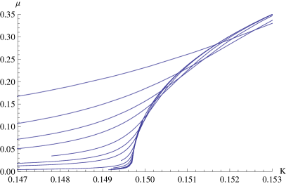
Figure 1: (Colour online) Magnetisation $\bar{\mu}(K)$ for lattice sizes $L=6,8,10,12,16,20,24,32,40,48,56,60,64,80$.

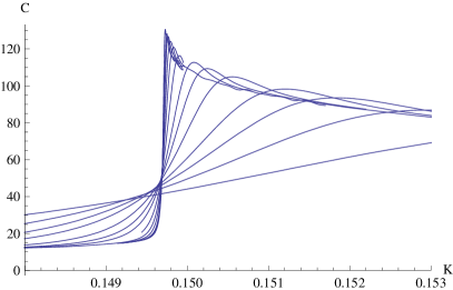
Figure 2: (Colour online) Specific heat $\mathcal{C}(K)$ for lattice sizes $L=6,8,10,12,16,20,24,32,40,48,56,60,64,80$.

III.1 Critical points and exponents

First we establish a high-precision estimate of the critical coupling $K_{c}$. This is done by determining the critical points for a number of different quantities, listed below, for each system size. The critical points in question are, with one exception, the locations of various maxima or minima of eg cumulants. To these points we fitted a simple scaling law of the form $c_{0}+c_{1}\,L^{-\lambda}$. By selecting points for $L\geq L_{\min}$ for different $L_{\min}$ we can then obtain several (for $L_{\min}=24,32,40$, with a few exceptions) different estimates of the fitting parameters. As a rule we received very good fits deeming a higher order correction term unnecessary. The sought parameter is of course $c_{0}$. Taking the median of these gives a final estimate of $K_{c}$ for that particular quantity. Repeating this for all quantities, a grand total of 15, allows us to make a statistical analysis of them. We have used the median as the estimate, with the first and third quartile as error estimates. In short, we take the median of the medians, very much like in Häggkvist et al. (2007).

The points scale very nicely with the linear order using only the simple expression above, see Figure 3. The resulting estimate is $K_{c}=0.1496947\pm 5\!\cdot\!10^{-7}$. This falls inside the by now rather old estimate $K_{c}=0.14965\pm 5\!\cdot\!10^{-5}$ found in Gaunt et al. (1979) and agrees with the estimate from Bittner et al. (2002).

The critical points in question are the locations of the following; the maximum of the specific heat $\mathcal{C}$ and susceptibility $\bar{\chi}$, maximum and minimum of the cumulants $c_{3}(E)/n$, $c_{3}(|M|)/n$, $(c_{4}(E)-3\,c_{2}(E))/n$ and $(c_{4}(|M|)-3\,c^{2}_{2}(|M|))/n$, maximum of $\partial\bar{\mu}/\partial K$, $\partial\ln\bar{\mu}/\partial K$, $\partial\ln\chi/\partial K$ and $\partial\mathcal{Q}/\partial K$, where $\mathcal{Q}$ is the Binder cumulant $1-\left<M^{4}\right>/3\,\left<M^{2}\right>^{2}$ and finally the crossing point between $\mathcal{Q}_{L}$ and $\mathcal{Q}_{L/2}$. See eg Ferrenberg and Landau (1991) for a discussion of the last four quantities.

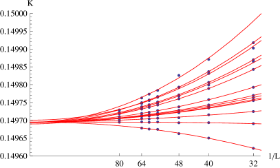
Figure 3: (Colour online) The critical points vs $1/L$ with fitted curves.

The expression above also provides us with estimates of the exponent $\nu$. The location of a critical point $K^{*}_{L}$ should deviate from $K_{c}$ as roughly $K^{*}_{L}-K_{c}\sim L^{-1/\nu}$, again see Ferrenberg and Landau (1991). Repeating the median-of-the-medians approach gives $\lambda=1/\nu=2.00\pm 0.03$ where the bounds are again based on the 1st and 3rd quartile, thus rendering us $\nu=0.50\pm 0.01$. The Josephson inequality tells us that $\alpha\geq 2-D\nu$, and hence our midpoint estimate gives $\alpha\geq 0\pm 0.04$ for $D=4$, since $\alpha=0$ Sokal (1979) our data is in good agreement with the rigorous results. Similarly an estimate of $\beta=0.50$ is found, and the mean-field value is $\beta=\frac{1}{2}$.

Having established an estimate of $K_{c}$ we can now estimate the internal energy $\mathcal{U}_{L}(K_{c})$ and again fit the scaling formula above to these data for $L_{\min}=24,32,40$. The different $c_{0}$, and thus the asymptotic values of $\mathcal{U}_{c}$, end up inside the interval $0.77053\pm 4\!\cdot\!10^{-5}$.

III.2 Critical values

Our aim is now to try to distinguish between the two possible scenarios, either we have a logarithmic singularity or the specific heat is bounded at $T_{c}$. We attempt to do this by making least-squares fits to the data for two different forms of the fitting function.

According to scaling theory, see Brézin et al. (1976), the maximum specific heat $\mathcal{C}_{\max}$ is proportional to $\sqrt[3]{\ln L}$. For $L\geq 12$ this seems plausible given our data. In Figure 4 we show $\mathcal{C}_{\max}$ versus $\sqrt[3]{\ln L}$ together with a fitted straight line, $y=115\,x-56.7$, and indeed they line up rather convincingly. The reader should note that $\mathcal{C}_{\max}$ grows very slowly indeed.

For the bounded scenario we try a fit where $\mathcal{C}_{\max}$ is proportional to a power of $L$. A least-squares fit of both constant and exponent gives $150.49+180.5L^{-0.496}$. We show this in the inset of Figure 4. The fact that the exponent is negative would of course mean that the specific heat is finite in the limit.

For both models there is some variation in the coefficients and the exponent if one makes the fit to different subsets of the data points, but no drastic changes. An attempt with evaluating the specific heat and the susceptibility at the asymptotic $K_{c}$ for each linear size instead gave a very similar behaviour to that of their maximum value.

To the eye both fitting functions work reasonably well and we simply find that the canonical ensemble data can not strongly distinguish the two scenarios.

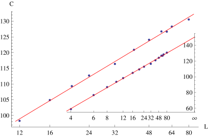
Figure 4: (Colour online) $\mathcal{C}_{\max}$ vs $\sqrt[3]{\ln L}$ and $L^{-0.496}$ (inset), together with the fitted curves.

IV Combinatorial quantities

With regards to the microcanonical ensemble the two scenarios will be that either $K^{\prime}(U)$ goes to 0 at $U_{c}$ or it converges to a finite positive value

Figure 5 shows the microcanonical quantity $K(U)$ and in Figure 6 its derivative is shown, both together with zoomed-in versions near the critical energy $U_{c}$. Most of the sampling was done for energies close to the critical one for the given value of $L$ so the curves become noisier further away from $U_{c}$.

The minima do not at all seem to approach zero as they do for $d=2$ Häggkvist et al. (2004b) and $d=3$ Häggkvist et al. (2007). In fact the behaviour here is qualitatively different in that the values are actually increasing rather than decreasing.

It is known, see e.g. Häggkvist et al. (2004a), that the specific heat corresponds to $1/K^{\prime}(U)$. Thus $\lim_{U\to U_{c}}K^{\prime}(U)=0$ if and only if $\lim_{K\to K_{c}}\mathcal{C}(K)=\infty$. Figure 7 shows the minima versus $1/L$ together with a fitted line $y=0.00419-0.0151\,x$, suggesting that the minimum approaches a maximum $0.00419$.

The optimal exponent of $1/L$, naturally, depends to some extent on which data points are used. Using a least-squares fit to different subsets of the data for $L\geq 6$ gives exponents between (roughly) $0.9$ and $1.5$. More specifically, if we check all subsets of the data with $L\geq 6$ on between 10 and 12 points a median exponent of $1.25$ is received and for $c_{0}$ the median value was $0.00406$ with first and third quartiles $0.00402$ and $0.00413$ respectively. The extremal values for $c_{0}$ are $0.0038$ and $0.0044$. If we instead use all the data points for $L\geq 8$ we obtain the exponent $\lambda=1.147$ and $c_{0}=0.00411$.

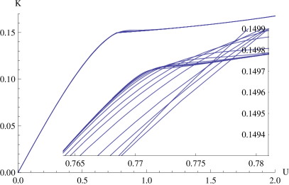
Figure 5: (Colour online) Coupling $K(U)$ for $L\geq 6$.

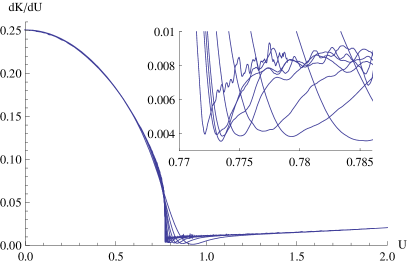
Figure 6: (Colour online) Coupling $K^{\prime}(U)$ for $L\geq 6$.

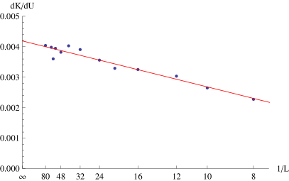
Figure 7: (Colour online) The minimum of $K^{\prime}(U)$ vs $1/L$, together with the fitted curve.

V Conclusions

We have studied the two proposed scenarios for the critical behaviour of the specific heat of the 4-dimensional Ising model. This has been done in both the canonical and the microcanonical ensembles. We have found that for the given lattice sizes the canonical ensemble can not conclusively distinguish between the two scenarios, and in an attempt to circumvent this we have instead turned to the microcanonical ensemble.

There are two reasons for why the microcanonical ensemble could give clearer results in this situation, the first predicted and the second unexpected.

First, the canonical ensemble is expected to have larger finite size effects than the microcanonical ensemble. To see this we may consider an idealised example where, for a finite system, $S(U)$ at each energy $U$ is identical to the limit as $n\rightarrow\infty$. Here the density of states has no finite size effects at all, apart from only being defined at certain discrete set of values of $U$. However because of the discrete energies there will still be finite-size effects in the corresponding canonical ensemble.

Secondly, a divergent specific heat means that $K^{\prime}(U)$ goes to 0 at $U_{c}$, and as we have found the minimum value of $K^{\prime}(U)$ is actually increasing rather than decreasing. This gives us a qualitative signal, rather than a weak quantitative one, that the specific heat actually converges to a finite value.

Our conclusion is that either much larger systems are needed to see the asymptotic behaviour of this model, and this possibility can only be ruled out by a rigorous convergence result, or the specific heat is in fact bounded at $U_{c}$, thus contradicting the renormalization theory prediction.

References

- Aizenman (1981) M. Aizenman, Phys. Rev. Lett. 47, 1 (1981), ISSN 0031-9007.
- Aizenman (1982) M. Aizenman, Comm. Math. Phys. 86, 1 (1982), ISSN 0010-3616.
- Sokal (1979) A. D. Sokal, Phys. Lett. A 71, 451 (1979).
- Bittner et al. (2002) E. Bittner, W. Janke, and H. Markum, Phys. Rev. D (3) 66, 024008, 8 (2002), ISSN 0556-2821.
- Blöte and Swendsen (1980) H. W. J. Blöte and R. H. Swendsen, Phys. Rev. B 22, 4481 (1980).
- Sanchez-Velasco (1987) E. Sanchez-Velasco, Journal of Physics A: Mathematical and General 20, 5033 (1987), URL http://stacks.iop.org/0305-4470/20/5033.
- Hellmund and Janke (2006) M. Hellmund and W. Janke, Physical Review B (Condensed Matter and Materials Physics) 74, 144201 (pages 9) (2006), URL http://link.aps.org/abstract/PRB/v74/e144201.
- Cea et al. (2005) P. Cea, M. Consoli, and L. Cosmai (2005), eprint hep-lat/0501013.
- Stevenson (2005) P. M. Stevenson, Nuclear Phys. B 729, 542 (2005), ISSN 0550-3213.
- Balog et al. (2006) J. Balog, F. Niedermayer, and P. Weisz, Nuclear Phys. B 741, 390 (2006), ISSN 0550-3213.
- Häggkvist et al. (2004a) R. Häggkvist, A. Rosengren, D. Andrén, P. Kundrotas, P. H. Lundow, and K. Markström, J. Statist. Phys. 114, 455 (2004a).
- Häggkvist et al. (2007) R. Häggkvist, A. Rosengren, P. H. Lundow, K. Markström, D. Andrén, and P. Kundrotas, Adv. Phys. 56, 653 (2007).
- Wolff (1989) U. Wolff, Phys. Rev. Lett 62, 361 (1989).
- (14) P. H. Lundow and K. Markström, arXiv:cond-mat/0612465.
- Ferrenberg and Landau (1991) A. M. Ferrenberg and D. P. Landau, Phys. Rev. B 44, 5081 (1991).
- Gaunt et al. (1979) D. S. Gaunt, M. F. Sykes, and S. McKenzie, J. Phys. A 12, 871 (1979).
- Brézin et al. (1976) E. Brézin, J. C. Le Guillou, and J. Zinn-Justin, in Phase transitions and critical phenomena, Vol. 6 (Academic Press, London, 1976), pp. 125–247.
- Häggkvist et al. (2004b) R. Häggkvist, A. Rosengren, D. Andrén, P. Kundrotas, P. H. Lundow, and K. Markström, Phys. Rev. E 69, 046104 (2004b).