Spherical Collapse in covariant Galileon theory

Emilio Bellini Dipartimento di Fisica e Astronomia “G. Galilei”, Università degli Studi di Padova, via Marzolo 8, I-35131, Padova, Italy
INFN, Sezione di Padova, via Marzolo 8, I-35131, Padova, Italy
emilio.bellini@pd.infn.it
   Nicola Bartolo Dipartimento di Fisica e Astronomia “G. Galilei”, Università degli Studi di Padova, via Marzolo 8, I-35131, Padova, Italy
INFN, Sezione di Padova, via Marzolo 8, I-35131, Padova, Italy
nicola.bartolo@pd.infn.it
   Sabino Matarrese Dipartimento di Fisica e Astronomia “G. Galilei”, Università degli Studi di Padova, via Marzolo 8, I-35131, Padova, Italy
INFN, Sezione di Padova, via Marzolo 8, I-35131, Padova, Italy
sabino.matarrese@pd.infn.it
Abstract

In this paper we study the evolution of a spherical matter overdensity in the context of the recently introduced Galileon field theory. Our analysis considers the complete covariant Lagrangian in four dimensions. This theory is composed by a potential and a standard kinetic term, a cubic kinetic term and two additional terms that include the coupling between the Galileon and the metric, to preserve the original properties of Galileons also in curved space-times. Here we extend previous studies, which considered both the quintessence and the cubic terms, by focussing on the role of the last two terms. The background evolution we consider is driven by a tracker solution. Studying scalar perturbations in the non-linear regime, we find constraints on the parameter of the model. We will show how the new terms contribute to the collapse phase and how they modify physical parameters, such as the linearized density contrast and the virial overdensity. The results show that the Galileon modifies substantially the dynamics of the collapse, thus making it possible to observationally constrain the parameters of this theory.

Keywords: Modified gravity, Galileon, Spherical Collapse, Cosmological Perturbations

1 Introduction

The discovery that the Universe underwent a phase of accelerated expansion at late times, through the study of the distance-redshift relation of type-Ia Supernovae (SNIa) [1, 2, 3], opened a new scenario for theoretical cosmology: the possibility to live in a Universe whose dynamics is presently driven by a component responsible for an “obscure” repulsive force, which has been dubbed Dark Energy (DE). Such a component should fill 74%percent7474\% of the energy budget of the universe, and it can be obtained by either just considering a non-zero cosmological constant term (ΛCDMΛCDM\Lambda\textrm{CDM} model). This model fits very well observational data, but, up to now, it is impossible to give a physical meaning to the tiny value of ΛΛ\Lambda required to explain dark energy. Thus, cosmologists explored alternative theories by e.g, modifying the Einstein-Hilbert action:

S=Mpl22d4xgR+d4xM,𝑆superscriptsubscript𝑀pl22superscriptd4𝑥𝑔𝑅superscriptd4𝑥subscript𝑀S=\frac{M_{\rm pl}^{2}}{2}\int{\rm d}^{4}x\sqrt{-g}\,R+\int{\rm d}^{4}x\,{\cal L}_{M}\,, (1)

where Mplsubscript𝑀plM_{\rm pl} represents the reduced Planck mass. Models that have been proposed are scalar-tensor theories [4], f(R)𝑓𝑅f(R) gravity (for a review see [5]), massive gravity (see [6]), Brane-World models (e.g. [7]) and others.

Recently, a new class of theories was introduced by Nicolis et al. [8], the so-called Galileon [9, 10, 11, 12, 13, 14, 15, 16, 17, 18, 19, 20, 21, 22, 23, 24, 25]. This model was constructed as an effective field theory, which is based upon and aims at extending the Dvali-Gabadadze-Porratti model (DGP) [26]. It is interesting because it solves ghost instabilities, which plague DGP, and has a screening mechanism that allows to satisfy the bounds coming from solar system experiments. To avoid the appearance of ghosts it is important to keep the equation of motion up to second-order in time-derivatives. Unfortunately, in the original model, this property was respected only in flat space-time. The works by Deffayet et al. [27, 28] found a way to generalize Galileons to curved space-time. To do this, it is necessary to add some extra terms which couple the scalar field with curvature terms. The result is a scalar-tensor theory in which the action, in flat space-time, is invariant under Galilean symmetry (μϕμϕ+bμsubscript𝜇italic-ϕsubscript𝜇italic-ϕsubscript𝑏𝜇\partial_{\mu}\phi\rightarrow\partial_{\mu}\phi+b_{\mu}).

Even though in this paper we study the effects of the late-time cosmic acceleration produced by the scalar field, adopting the spherical collapse model, it is worth mentioning that the importance of the Galileon field also relis on the fact that it can inspire some “inflationary-like” model, e.g. [29] (even though this theory does not respect the galilean symmetry).

In this paper we will use the background evolution given by the tracker solution found in [30], which ensures a de Sitter (dS) stable point. While it is shown that the cosmology of the Galileon lets the universe expands accelerating at late-times, in this paper we will show that at short distances we can satisfy solar system constraints via the Vainshtein mechanism [31, 32], see also [33] for a discussion in the most general second order scalar-tensor theory. This mechanism can work in massive gravity, but also in different contexts. An example is DGP theory, which possesses a Vainshtein radius defined by rV=(rsrc2)1/3subscript𝑟𝑉superscriptsubscript𝑟𝑠superscriptsubscript𝑟𝑐213r_{V}=(r_{s}r_{c}^{2})^{1/3} (where rssubscript𝑟𝑠r_{s} is the Schwarzschild radius of the source, rcsubscript𝑟𝑐r_{c} is a coupling constant which defines the crossover scale between a 5-dimensional Minkowsky space and the embedded 4-dimensional space-time). Even if the Galileon does not already have a well-defined Vainshtein radius, we will show how to recover a valid definition of it. In fact, as in DGP, instead of a massive graviton, this mechanism can also work using non-linear self-interaction terms of the scalar field (as ϕ(ϕ)2italic-ϕsuperscriptitalic-ϕ2\Box\phi{\left(\nabla\phi\right)}^{2}).

The spherical collapse model (e.g. [34, 35, 36]) studies the evolution of a spherical Dark Matter (DM) overdensity to explain the formation of cosmic structures. We will use the top-hat approximation, taking into account the energy non-conservation problem noted in [35]. This problem affects theories with a time-dependent dark energy component, and it can substantially modify the virialisation process.

The paper is organized as follows. In Section 2 we define the action we are assuming and we obtain the equations of motion. In Section 3 we briefly review the background evolution of a Friedmann-Lemaître-Robertson-Walker universe (FRLW) following a tracker solution found in [30]. In Section 4 we study scalar perturbations, both in the linear and non-linear regime. We also study the Vainshtein mechanism, and discuss the existence of a solution for the Galileon field in the non-linear regime. In Section 5 we study the dynamics of a spherical top-hat matter perturbation. In Section 6 we discuss our main results. In A and B we give some useful functions.

Throughout the paper we adopt units c==G=1𝑐Planck-constant-over-2-pi𝐺1c=\hbar=G=1, except where explicitly indicated; our signature is (,+,+,+)(-,+,+,+).

2 Action and Field equations

Let us start with the covariant action for the Galileon model non-minimally coupled to the metric [30]:

S=d4xg[Mpl22R+12i=15cii]+d4xM,𝑆superscriptd4𝑥𝑔delimited-[]superscriptsubscript𝑀pl22𝑅12superscriptsubscript𝑖15subscript𝑐𝑖subscript𝑖superscriptd4𝑥subscript𝑀S=\int{\rm d}^{4}x\sqrt{-g}\,\left[\frac{M_{\rm pl}^{2}}{2}R+\frac{1}{2}\sum_{i=1}^{5}c_{i}{\cal L}_{i}\right]+\int{\rm d}^{4}x\,{\cal L}_{M}\,, (2)

where cisubscript𝑐𝑖c_{i} are dimensionless constants. We consider Msubscript𝑀{\cal L}_{M} as the Lagrangian of a pressurless perfect fluid with density ρ𝜌\rho. The five Lagrangian densities for the scalar field are:

1subscript1\displaystyle{\cal L}_{1} =\displaystyle= M3ϕsuperscript𝑀3italic-ϕ\displaystyle M^{3}\phi (3)
2subscript2\displaystyle{\cal L}_{2} =\displaystyle= (ϕ)2superscriptitalic-ϕ2\displaystyle(\nabla\phi)^{2} (4)
3subscript3\displaystyle{\cal L}_{3} =\displaystyle= (ϕ)(ϕ)2/M3italic-ϕsuperscriptitalic-ϕ2superscript𝑀3\displaystyle(\square\phi)(\nabla\phi)^{2}/M^{3} (5)
4subscript4\displaystyle{\cal L}_{4} =\displaystyle= (ϕ)2[2(ϕ)22ϕ;μνϕ;μνR(ϕ)2/2]/M6\displaystyle(\nabla\phi)^{2}\left[2(\square\phi)^{2}-2\phi_{;\mu\nu}\phi^{;\mu\nu}-R(\nabla\phi)^{2}/2\right]/M^{6} (6)
5subscript5\displaystyle{\cal L}_{5} =\displaystyle= (ϕ)2[(ϕ)33(ϕ)ϕ;μνϕ;μν+2ϕ;μνϕ;νρϕ;ρμ+\displaystyle(\nabla\phi)^{2}[(\square\phi)^{3}-3(\square\phi)\,\phi_{;\mu\nu}\phi^{;\mu\nu}+2{\phi_{;\mu}}^{\nu}{\phi_{;\nu}}^{\rho}{\phi_{;\rho}}^{\mu}+ (7)
6ϕ;μϕ;μνϕ;ρGνρ]/M9,\displaystyle-6\phi_{;\mu}\phi^{;\mu\nu}\phi^{;\rho}G_{\nu\rho}]/M^{9}\,,

where M𝑀M is a constant with dimensions of mass, and we defined its value as M3MplHdS2superscript𝑀3subscript𝑀plsuperscriptsubscript𝐻𝑑𝑆2M^{3}\equiv M_{\rm pl}H_{dS}^{2}. HdSsubscript𝐻dSH_{\rm dS} is the value of the Hubble parameter H(t)𝐻𝑡H(t) in a FRLW universe at the de Sitter fixed point. Indeed, as we will see, [30] found a tracker solution that ends at a stable point called “de Sitter point”, at which the energy density of the scalar field dominates. 1subscript1{\cal L}_{1} can be understood as a potential term and for this reason we set c1=0subscript𝑐10c_{1}=0, since we are interested in analyzing the contribution of the new kinetic terms (the case in which a standard minimally coupled scalar field is introduced in the field equations was already studied in [37]). Moreover, with this choice we can employ the tracker solution given in [30], that is not admitted if c10subscript𝑐10c_{1}\neq 0. 2subscript2{\cal L}_{2} is the standard kinetic term. 3subscript3{\cal L}_{3} comes directly from the decoupling limit of DGP theory. 4subscript4{\cal L}_{4} and 5subscript5{\cal L}_{5} provide the full generalization of an action containing at most second derivatives with respect to Galilean shift symmetry in a flat space-time. The coupling between ϕitalic-ϕ\phi and the curvature tensors are required to construct a Lagrangian free of third or higher-order derivatives in the equations of motion.

Varying this action with respect to the metric gμνsubscript𝑔𝜇𝜈g_{\mu\nu} and the scalar field ϕitalic-ϕ\phi we obtain the equations of motion. For the metric:

Gμν=Mpl2[Tμν(m)+Tμν(ϕ)],subscript𝐺𝜇𝜈superscriptsubscript𝑀pl2delimited-[]subscriptsuperscript𝑇𝑚𝜇𝜈subscriptsuperscript𝑇italic-ϕ𝜇𝜈G_{\mu\nu}=M_{\rm pl}^{-2}\left[T^{(m)}_{\phantom{(m)}\mu\nu}+T^{(\phi)}_{\phantom{(\phi)}\mu\nu}\right]\;, (8)

where

Tμν(ϕ)=i=15ciTμν(i),subscriptsuperscript𝑇italic-ϕ𝜇𝜈superscriptsubscript𝑖15subscript𝑐𝑖subscriptsuperscript𝑇𝑖𝜇𝜈T^{(\phi)}_{\phantom{(m)}\mu\nu}=\sum_{i=1}^{5}c_{i}T^{(i)}_{\phantom{(m)}\mu\nu}\;, (9)

the terms Tμν(i)subscriptsuperscript𝑇𝑖𝜇𝜈T^{(i)}_{\phantom{(i)}\mu\nu} being listed in A. Instead, varying with respect to the scalar field, we obtain

i=15ciξ(i)=0,superscriptsubscript𝑖15subscript𝑐𝑖superscript𝜉𝑖0\sum_{i=1}^{5}c_{i}\xi^{(i)}=0\;, (10)

where ξ(i)superscript𝜉𝑖\xi^{(i)} are also listed in A.

3 Background evolution

From Eqs. (8) and (10) we can study the background evolution in an expanding FLRW universe with scale factor a(t)𝑎𝑡a(t). Calling ϕϕ(t)italic-ϕitalic-ϕ𝑡\phi\equiv\phi(t) and ρρm(t)+ρr(t)𝜌subscript𝜌𝑚𝑡subscript𝜌𝑟𝑡\rho\equiv\rho_{m}(t)+\rho_{r}(t), the background scalar field and background matter and radiation density respectively, the field equations read

3Mpl2H2=ρϕ+ρm+ρr,3superscriptsubscript𝑀pl2superscript𝐻2subscript𝜌italic-ϕsubscript𝜌𝑚subscript𝜌𝑟\displaystyle 3M_{\rm pl}^{2}H^{2}=\rho_{\rm\phi}+\rho_{m}+\rho_{r}\,, (11)
3Mpl2H2+2Mpl2H˙=Pϕρr/3,3superscriptsubscript𝑀pl2superscript𝐻22superscriptsubscript𝑀pl2˙𝐻subscript𝑃italic-ϕsubscript𝜌𝑟3\displaystyle 3M_{\rm pl}^{2}H^{2}+2M_{\rm pl}^{2}\dot{H}=-P_{\rm\phi}-\rho_{r}/3\,, (12)

and

c2[3Hϕ˙+ϕ¨]3c3M3ϕ˙[3H2ϕ˙+H˙ϕ˙+2Hϕ¨]+18c4M6Hϕ˙2[3H2ϕ˙+\displaystyle c_{2}\left[3H\dot{\phi}+\ddot{\phi}\right]-\frac{3c_{3}}{M^{3}}\dot{\phi}\left[3H^{2}\dot{\phi}+\dot{H}\dot{\phi}+2H\ddot{\phi}\right]+\frac{18c_{4}}{M^{6}}H\dot{\phi}^{2}\left[3H^{2}\dot{\phi}+\right. (13)
+2H˙ϕ˙+3Hϕ¨]15c5M9H2ϕ˙3[3H2ϕ˙+3H˙ϕ˙+4Hϕ¨]=0,\displaystyle\left.+2\dot{H}\dot{\phi}+3H\ddot{\phi}\right]-\frac{15c_{5}}{M^{9}}H^{2}\dot{\phi}^{3}\left[3H^{2}\dot{\phi}+3\dot{H}\dot{\phi}+4H\ddot{\phi}\right]=0\;,

where

ρϕsubscript𝜌italic-ϕ\displaystyle\rho_{\rm\phi} \displaystyle\equiv c22ϕ˙2+3c3M3Hϕ˙345c42M6H2ϕ˙4+21c5M9H3ϕ˙5,subscript𝑐22superscript˙italic-ϕ23subscript𝑐3superscript𝑀3𝐻superscript˙italic-ϕ345subscript𝑐42superscript𝑀6superscript𝐻2superscript˙italic-ϕ421subscript𝑐5superscript𝑀9superscript𝐻3superscript˙italic-ϕ5\displaystyle-\frac{c_{2}}{2}\dot{\phi}^{2}+\frac{3c_{3}}{M^{3}}H\dot{\phi}^{3}-\frac{45c_{4}}{2M^{6}}H^{2}\dot{\phi}^{4}+\frac{21c_{5}}{M^{9}}H^{3}\dot{\phi}^{5}\,, (14)
Pϕsubscript𝑃italic-ϕ\displaystyle P_{\rm\phi} \displaystyle\equiv c22ϕ˙2c3M3ϕ˙2ϕ¨+3c42M6ϕ˙3[8Hϕ¨+(3H2+2H˙)ϕ˙]+subscript𝑐22superscript˙italic-ϕ2subscript𝑐3superscript𝑀3superscript˙italic-ϕ2¨italic-ϕlimit-from3subscript𝑐42superscript𝑀6superscript˙italic-ϕ3delimited-[]8𝐻¨italic-ϕ3superscript𝐻22˙𝐻˙italic-ϕ\displaystyle-\frac{c_{2}}{2}\dot{\phi}^{2}-\frac{c_{3}}{M^{3}}\dot{\phi}^{2}\ddot{\phi}+\frac{3c_{4}}{2M^{6}}\dot{\phi}^{3}[8H\ddot{\phi}+(3H^{2}+2\dot{H})\dot{\phi}]+ (15)
3c5M9Hϕ˙4[5Hϕ¨+2(H2+H˙)ϕ˙],3subscript𝑐5superscript𝑀9𝐻superscript˙italic-ϕ4delimited-[]5𝐻¨italic-ϕ2superscript𝐻2˙𝐻˙italic-ϕ\displaystyle-\frac{3c_{5}}{M^{9}}H\dot{\phi}^{4}[5H\ddot{\phi}+2(H^{2}+\dot{H})\dot{\phi}]\,,

are scalar field density and pressure, respectively.

As in [30], to study the background we work with the new variables

r1ϕ˙dSHdS/(ϕ˙H),r2(ϕ˙/ϕ˙dS)4/r1,Ωr=ρr/(3Mpl2H2),formulae-sequencesubscript𝑟1subscript˙italic-ϕdSsubscript𝐻dS˙italic-ϕ𝐻formulae-sequencesubscript𝑟2superscript˙italic-ϕsubscript˙italic-ϕdS4subscript𝑟1subscriptΩ𝑟subscript𝜌𝑟3superscriptsubscript𝑀pl2superscript𝐻2r_{1}\equiv\dot{\phi}_{\rm dS}H_{\rm dS}/(\dot{\phi}H)\,,\quad r_{2}\equiv(\dot{\phi}/\dot{\phi}_{\rm dS})^{4}/r_{1}\,,\quad\Omega_{r}=\rho_{r}/(3M_{\rm pl}^{2}H^{2})\,, (16)

where ϕ˙dSsubscript˙italic-ϕdS\dot{\phi}_{\rm dS} is the time derivative of the scalar field at the dS point. At this point Eqs. (11) and (12) becomes:

c2xdS2=6+9α12β,subscript𝑐2superscriptsubscript𝑥dS269𝛼12𝛽\displaystyle c_{2}x_{\rm dS}^{2}=6+9\alpha-12\beta\,, (17)
c3xdS3=2+9α9β,subscript𝑐3superscriptsubscript𝑥dS329𝛼9𝛽\displaystyle c_{3}x_{\rm dS}^{3}=2+9\alpha-9\beta\,, (18)

where xdSϕ˙dS/(HdSMpl)subscript𝑥dSsubscript˙italic-ϕdSsubscript𝐻dSsubscript𝑀plx_{\rm dS}\equiv\dot{\phi}_{\rm dS}/(H_{\rm dS}M_{\rm pl}). These equations give two conditions for the coefficients c2subscript𝑐2c_{2} and c3subscript𝑐3c_{3}. We also set αc4xdS4𝛼subscript𝑐4superscriptsubscript𝑥dS4\alpha\equiv c_{4}x_{\rm dS}^{4} and βc5xdS5𝛽subscript𝑐5superscriptsubscript𝑥dS5\beta\equiv c_{5}x_{\rm dS}^{5}; therefore our free parameters become α𝛼\alpha, β𝛽\beta and xdSsubscript𝑥dSx_{\rm dS}. For simplicity, the assumption xdS=1subscript𝑥dS1x_{\rm dS}=1 will be often used in the rest of the paper. An approximation we have done is HdSH0similar-to-or-equalssubscript𝐻dSsubscript𝐻0H_{\rm dS}\simeq H_{0}, where H0subscript𝐻0H_{0} is the value of the Hubble parameter today.

As we already mentioned, [30] found a stable tracker solution (r1=1subscript𝑟11r_{1}=1), which drives the universe expansion from the radiation-dominated epoch (r21much-less-thansubscript𝑟21r_{2}\ll 1, Ωr=1subscriptΩ𝑟1\Omega_{r}=1), through the matter-dominated epoch (r2=1subscript𝑟21r_{2}=1, Ωr1much-less-thansubscriptΩ𝑟1\Omega_{r}\ll 1), until the dS point (r2=1subscript𝑟21r_{2}=1, Ωr=0subscriptΩ𝑟0\Omega_{r}=0). Note that along r1=1subscript𝑟11r_{1}=1, Ωϕρϕ/(3Mpl2H2)=r2subscriptΩitalic-ϕsubscript𝜌italic-ϕ3superscriptsubscript𝑀pl2superscript𝐻2subscript𝑟2\Omega_{\phi}\equiv\rho_{\phi}/(3M_{\rm pl}^{2}H^{2})=r_{2}. Following this solution, Eqs. (12) and (10) with our new variables can be written as

r2=2r2(33r2+Ωr)1+r2,Ωr=Ωr(Ωr17r2)1+r2,formulae-sequencesuperscriptsubscript𝑟22subscript𝑟233subscript𝑟2subscriptΩ𝑟1subscript𝑟2superscriptsubscriptΩ𝑟subscriptΩ𝑟subscriptΩ𝑟17subscript𝑟21subscript𝑟2r_{2}^{\prime}=\frac{2r_{2}\left(3-3r_{2}+\Omega_{r}\right)}{1+r_{2}},\qquad\Omega_{r}^{\prime}=\frac{\Omega_{r}\left(\Omega_{r}-1-7r_{2}\right)}{1+r_{2}}\;, (19)

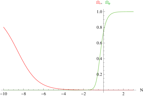
where primes denote differentiation w.r.t. N=lna𝑁𝑎N=\ln a. In Fig. 1 we show the numerical solution of these equations with boundary conditions Ωr0=4.8105subscriptΩsubscript𝑟04.8superscript105\Omega_{r_{0}}=4.8\cdot 10^{-5} and ΩΛ0=0.74subscriptΩsubscriptΛ00.74\Omega_{\Lambda_{0}}=0.74, where Ωr0subscriptΩsubscript𝑟0\Omega_{r_{0}} and ΩΛ0subscriptΩsubscriptΛ0\Omega_{\Lambda_{0}} are the density parameter values today, for the radiation and the dark energy component, respectively. These equations cannot be solved analytically; however we have found two analytic functions that approximate the numerical results with an accuracy better than 1.2%percent1.21.2\% at redshift z21less-than-or-similar-to𝑧21z\lesssim 21:

r2(N)1+[(1ΩΛ0)22ΩΛ01ΩΛ02ΩΛ04e6N+(1ΩΛ0)2ΩΛ0]e6N,similar-to-or-equalssubscript𝑟2𝑁1delimited-[]superscript1subscriptΩsubscriptΛ022subscriptΩsubscriptΛ01subscriptΩsubscriptΛ02subscriptΩsubscriptΛ04superscript𝑒6𝑁superscript1subscriptΩsubscriptΛ02subscriptΩsubscriptΛ0superscript𝑒6𝑁r_{2}(N)\simeq 1+\left[\frac{{(1-\Omega_{\Lambda_{0}})}^{2}}{2\Omega_{\Lambda_{0}}}-\frac{1-\Omega_{\Lambda_{0}}}{2\sqrt{\Omega_{\Lambda_{0}}}}\cdot\sqrt{4e^{6N}+\frac{{(1-\Omega_{\Lambda_{0}})}^{2}}{\Omega_{\Lambda_{0}}}}\right]\cdot e^{-6N}\,, (20)

and:

Ωr(N)2Ωr0eN(1ΩΛ0+4ΩΛ0e6N+(1ΩΛ0)2)1.similar-to-or-equalssubscriptΩ𝑟𝑁2subscriptΩsubscript𝑟0superscript𝑒𝑁superscript1subscriptΩsubscriptΛ04subscriptΩsubscriptΛ0superscript𝑒6𝑁superscript1subscriptΩsubscriptΛ021\Omega_{r}(N)\simeq 2\Omega_{r_{0}}e^{-N}{\left(1-\Omega_{\Lambda_{0}}+\sqrt{4\Omega_{\Lambda_{0}}e^{6N}+{(1-\Omega_{\Lambda_{0}})}^{2}}\right)}^{-1}\,. (21)
Refer to caption
Figure 1: In the figure we show the evolution of ΩrsubscriptΩ𝑟\Omega_{r} (red line) and ΩϕsubscriptΩitalic-ϕ\Omega_{\phi} (green line), functions of N=lna𝑁𝑎N=\ln a.

To study the stability of the solution r1(N)=1subscript𝑟1𝑁1r_{1}(N)=1, Eqs. (11), (12) and (13) can be expanded at linear order in perturbations δr1𝛿subscript𝑟1\delta r_{1}, δr2𝛿subscript𝑟2\delta r_{2} and δΩr𝛿subscriptΩ𝑟\delta\Omega_{r}. Thus, it can be obtained:

δr1(N)=9+Ωr(N)+3r2(N)2(1+r2(N))δr1(N),𝛿superscriptsubscript𝑟1𝑁9subscriptΩ𝑟𝑁3subscript𝑟2𝑁21subscript𝑟2𝑁𝛿subscript𝑟1𝑁{\delta r_{1}}^{\prime}(N)=-\frac{9+\Omega_{r}(N)+3r_{2}(N)}{2\left(1+r_{2}(N)\right)}\delta r_{1}(N)\,, (22)

which reads:

δr1(N)=δr1(0)exp[0N𝑑N9+Ωr(N)+3r2(N)2(1+r2(N))]f0e92N.𝛿subscript𝑟1𝑁𝛿subscript𝑟10superscriptsubscript0𝑁differential-dsuperscript𝑁9subscriptΩ𝑟superscript𝑁3subscript𝑟2superscript𝑁21subscript𝑟2superscript𝑁subscript𝑓0superscript𝑒92𝑁\delta r_{1}(N)=\delta r_{1}(0)\exp\left[-\int_{0}^{N}dN^{\prime}\frac{9+\Omega_{r}(N^{\prime})+3r_{2}(N^{\prime})}{2\left(1+r_{2}(N^{\prime})\right)}\right]\leq f_{0}\,e^{-\frac{9}{2}N}\,. (23)

f0subscript𝑓0f_{0} is a finite integration constant, and this relation proves that any solution that approaches r1(N)=1subscript𝑟1𝑁1r_{1}(N)=1, finally reaches it. Indeed, in the rest of the paper, we shall suppose that at least after the matter-dominated epoch the evolution of the universe can be described by δr11much-less-than𝛿subscript𝑟11\delta r_{1}\ll 1.

In [30], the authors also find constraints on the parameters α𝛼\alpha and β𝛽\beta (assuming xdS=1subscript𝑥dS1x_{\rm dS}=1). These constraints follow from the requirement of ghost avoidance. They study scalar (S) and tensor (T) perturbations, expanding the action Eq. (2) at second-order in perturbation theory (see [38, 39], for the complete procedure), finding conditions for the sign of the kinetic term (QSsubscript𝑄𝑆Q_{S} and QTsubscript𝑄𝑇Q_{T}) and the squared sound speed (cS2superscriptsubscript𝑐𝑆2c_{S}^{\phantom{S}2} and cT2superscriptsubscript𝑐𝑇2c_{T}^{\phantom{T}2}). Thus, in every epoch we have four conditions that must be satisfied. Reminding that α𝛼\alpha and β𝛽\beta are constants, we can find a region of parameter space where no ghost modes exist. This area is bounded by the analytic functions

{α>2βα<2β+2/3α<12β9β2α>12/13β+10/13.cases𝛼2𝛽𝛼2𝛽23𝛼12𝛽9𝛽2𝛼1213𝛽1013\left\{\begin{array}[]{l}\alpha>2\,\beta\\ \alpha<2\,\beta+2/3\\ \alpha<12\,\sqrt{\beta}-9\,\beta-2\\ \alpha>12/13\,\beta+10/13\,.\end{array}\right. (24)

4 Cosmological perturbations

In this section we study the evolution of scalar perturbations on sub-horizon scales. Our work focuses on the dynamics of a spherically symmetric perturbed metric. Let us choose the conformal Newtonian gauge,

ds2=(1+2Ψ)dt2+a2(t)(1+2Φ)δijdxidxj.𝑑superscript𝑠212Ψ𝑑superscript𝑡2superscript𝑎2𝑡12Φsubscript𝛿𝑖𝑗𝑑superscript𝑥𝑖𝑑superscript𝑥𝑗ds^{2}=-(1+2\Psi)dt^{2}+a^{2}(t)(1+2\Phi)\delta_{ij}dx^{i}dx^{j}\,. (25)

Perturbations of the energy density and the scalar field are given by

ρ(x,t)ρ0(t)+δρ(x,t)ϕ(x,t)ϕ0(t)+φ(x,t).formulae-sequence𝜌𝑥𝑡subscript𝜌0𝑡𝛿𝜌𝑥𝑡italic-ϕ𝑥𝑡subscriptitalic-ϕ0𝑡𝜑𝑥𝑡\rho(\vec{x},t)\equiv\rho_{0}(t)+\delta\rho(\vec{x},t)\qquad\phi(\vec{x},t)\equiv\phi_{0}(t)+\varphi(\vec{x},t)\,. (26)

In the following we will drop the suffix “00”. In this regime there are two valid approximations that simplify the field equations. The first one is the sub-horizon approximation 𝒪(2Φ/a2)𝒪(H2Φ)much-greater-than𝒪superscript2Φsuperscript𝑎2𝒪superscript𝐻2Φ\mathcal{O}(\nabla^{2}\Phi/a^{2})\gg\mathcal{O}(H^{2}\Phi). The second one is the quasi-static approximation, which allows us to neglect time derivatives of perturbations compared with space derivatives, assuming we are working with non-relativistic matter at short distances.

4.1 Linear perturbation theory

Replacing physical gradients with comoving gradients, at linear order Eqs. (8) and (10) become (\nabla denotes a spatial gradient):

(2Mpl2+ϕ˙2γ1(t))2Φ=δρ+γ2(t)2φ,2superscriptsubscript𝑀pl2superscript˙italic-ϕ2subscript𝛾1𝑡superscript2Φ𝛿𝜌subscript𝛾2𝑡superscript2𝜑\left(2M_{\rm pl}^{2}+\dot{\phi}^{2}\gamma_{1}(t)\right)\nabla^{2}\Phi=-\delta\rho+\gamma_{2}(t)\nabla^{2}\varphi\,, (27)
(2Mpl2+3γ3(t))2Φ+(2Mpl2+ϕ˙2γ1(t))2Ψ=3γ4(t)2φ,2superscriptsubscript𝑀pl23subscript𝛾3𝑡superscript2Φ2superscriptsubscript𝑀pl2superscript˙italic-ϕ2subscript𝛾1𝑡superscript2Ψ3subscript𝛾4𝑡superscript2𝜑\left(2M_{\rm pl}^{2}+3\gamma_{3}(t)\right)\nabla^{2}\Phi+\left(2M_{\rm pl}^{2}+\dot{\phi}^{2}\gamma_{1}(t)\right)\nabla^{2}\Psi=3\gamma_{4}(t)\nabla^{2}\varphi\,, (28)

and

γ5(t)2φ+γ2(t)2Ψ+3γ4(t)2Φ=0,subscript𝛾5𝑡superscript2𝜑subscript𝛾2𝑡superscript2Ψ3subscript𝛾4𝑡superscript2Φ0\gamma_{5}(t)\nabla^{2}\varphi+\gamma_{2}(t)\nabla^{2}\Psi+3\gamma_{4}(t)\nabla^{2}\Phi=0\;, (29)

where γi(t)subscript𝛾𝑖𝑡\gamma_{i}(t) are functions of the background, whose explicit form is given in B.

It is important to note that one of the differences between these equations and those for the kinetic braiding model studied in [36] is the presence of an anisotropic stress in the RHS of Eq. (28).

Manipulating Eqs. (27) and (28), we obtain the modified Poisson equation

(2Mpl2+ϕ˙2γ1)22Mpl2+3γ32Ψ=δρ[γ23γ52Mpl2+ϕ˙2γ12Mpl2+3γ3]2φ.superscript2superscriptsubscript𝑀pl2superscript˙italic-ϕ2subscript𝛾122superscriptsubscript𝑀pl23subscript𝛾3superscript2Ψ𝛿𝜌delimited-[]subscript𝛾23subscript𝛾52superscriptsubscript𝑀pl2superscript˙italic-ϕ2subscript𝛾12superscriptsubscript𝑀pl23subscript𝛾3superscript2𝜑\frac{{\left(2M_{\rm pl}^{2}+\dot{\phi}^{2}\gamma_{1}\right)}^{2}}{2M_{\rm pl}^{2}+3\gamma_{3}}\nabla^{2}\Psi=\delta\rho-\left[\gamma_{2}-3\gamma_{5}\frac{2M_{\rm pl}^{2}+\dot{\phi}^{2}\gamma_{1}}{2M_{\rm pl}^{2}+3\gamma_{3}}\right]\nabla^{2}\varphi\,. (30)

Using Eqs. (29), (27) and (30), the differential equation for the evolution of the scalar field takes the form

2φ=A(t)δρ(t,r),superscript2𝜑𝐴𝑡𝛿𝜌𝑡𝑟\nabla^{2}\varphi=A(t)\,\delta\rho(t,\vec{r}), (31)

where

A(t)γ2(t)γ7(t)3γ4(t)γ6(t)γ2(t)2γ7(t)γ5(t)γ6(t)26γ2(t)γ4(t)γ6(t),𝐴𝑡subscript𝛾2𝑡subscript𝛾7𝑡3subscript𝛾4𝑡subscript𝛾6𝑡subscript𝛾2superscript𝑡2subscript𝛾7𝑡subscript𝛾5𝑡subscript𝛾6superscript𝑡26subscript𝛾2𝑡subscript𝛾4𝑡subscript𝛾6𝑡A(t)\equiv\frac{\gamma_{2}(t)\gamma_{7}(t)-3\gamma_{4}(t)\gamma_{6}(t)}{{\gamma_{2}(t)}^{2}\gamma_{7}(t)-\gamma_{5}(t){\gamma_{6}(t)}^{2}-6\gamma_{2}(t)\gamma_{4}(t)\gamma_{6}(t)}\;, (32)

with γ6(t)(2Mpl2+ϕ˙2γ1(t))subscript𝛾6𝑡2superscriptsubscript𝑀pl2superscript˙italic-ϕ2subscript𝛾1𝑡\gamma_{6}(t)\equiv\left(2M_{\rm pl}^{2}+\dot{\phi}^{2}\gamma_{1}(t)\right) and γ7(t)(2Mpl2+3γ3(t))subscript𝛾7𝑡2superscriptsubscript𝑀pl23subscript𝛾3𝑡\gamma_{7}(t)\equiv\left(2M_{\rm pl}^{2}+3\gamma_{3}(t)\right). Considering a spherically symmetric object of radius RSsubscript𝑅𝑆R_{S}, we can easily integrate Eq. (31) to obtain an analytic expression for the evolution of the scalar field. Defining m(t,r)4π0rdrr2δρ𝑚𝑡𝑟4𝜋superscriptsubscript0𝑟superscriptdrsuperscriptsuperscriptr2𝛿𝜌m(t,r)\equiv 4\pi\int_{0}^{r}\rm dr^{\prime}{r^{\prime}}^{2}\delta\rho, we obtain

dφdr=A(t)m(t,r)4πr2+Cr2,d𝜑dr𝐴𝑡𝑚𝑡𝑟4𝜋superscript𝑟2𝐶superscript𝑟2\frac{\rm d\varphi}{\rm dr}=\frac{A(t)\,m(t,r)}{4\pi r^{2}}+\frac{C}{r^{2}}\,, (33)

where C𝐶C is an integration constant that, outside the source, can be viewed as an increase in Msm(t,RS)subscript𝑀𝑠𝑚𝑡subscript𝑅𝑆M_{s}\equiv m(t,R_{S}). While this term is present in φsuperscript𝜑\varphi^{\prime}, it does not enter in 2φsuperscript2𝜑\nabla^{2}\varphi, so that the gravitational potential is not affected by our choice of C𝐶C. Therefore, for our purposes we can set C=0𝐶0C=0.

4.2 Vainshtein mechanism in the linear regime

The Vainshtein mechanism works by screening the effects of the scalar field on the gravitational potential at small distances, so that one can satisfy the constraints coming from solar-system tests, while preserving the accelerated expansion of the universe on cosmological scales. The difference between this mechanism and the Chamaleon one is that the first also works by using non-linearities of the perturbations to this aim. At large distances (rrVmuch-greater-than𝑟subscript𝑟𝑉r\gg r_{V}, where rVsubscript𝑟𝑉r_{V} is the Vainshtein radius of the source) linear terms of the scalar field become dominant, while for rrVmuch-less-than𝑟subscript𝑟𝑉r\ll r_{V} non-linear terms become dominant (these terms will be shown in Eqs. (4.3), (4.3) and (4.3)). This is called “self-screening effect”. A discussion about the magnitude of the Vainshtein radius (rVsubscript𝑟𝑉r_{V}) of a spherically symmetric source will be given later (Sec. 4.4).

A first approach is to study within the linear approximation the contribution of the scalar field to the gravitational potential. Recalling Eq. (30), to have a qualitative knowledge that outside the Vainshtein radius the scalar field drives the late time cosmic acceleration, we have to compare the contribution of the gravitational with the scalar field intensity [40]. Indeed, our request is that the two are comparable:

φ(r)Ψ(r)1.similar-to-or-equalssuperscript𝜑𝑟superscriptΨ𝑟1\frac{\varphi^{\prime}(r)}{\Psi^{\prime}(r)}\simeq 1\,. (34)

It can be shown that the above ratio is a monotone function, which starts from 0similar-to-or-equalsabsent0\simeq 0 during the radiation-matter-dominated epoch. At the dS point, recalling Eq. (31) with xdS=1subscript𝑥dS1x_{\rm dS}=1, we obtain

|φ(r)Ψ(r)|dS=|A(tdS)4π|=|124πMpl(2βα)|.subscriptsuperscript𝜑𝑟superscriptΨ𝑟dS𝐴subscript𝑡dS4𝜋124𝜋subscript𝑀pl2𝛽𝛼{\left|\frac{\varphi^{\prime}(r)}{\Psi^{\prime}(r)}\right|}_{\rm dS}=\left|\frac{A(t_{\rm dS})}{4\pi}\right|=\left|\frac{1}{24\pi M_{\rm pl}(2\beta-\alpha)}\right|\,. (35)

Taking into account the region in the plane (xdS=1,β,α)subscript𝑥dS1𝛽𝛼(x_{\rm dS}=1,\beta,\alpha) bounded by the no-ghost condition (24), it can be shown that the magnitude of the last ratio at the dS point is bounded by

142π<|φ(r)Ψ(r)|dS<+142𝜋subscriptsuperscript𝜑𝑟superscriptΨ𝑟dS\frac{1}{4\sqrt{2\pi}}<{\left|\frac{\varphi^{\prime}(r)}{\Psi^{\prime}(r)}\right|}_{\rm dS}<+\infty (36)

This result means that the contribution of the scalar field at the dS point on scales rrVmuch-greater-than𝑟subscript𝑟𝑉r\gg r_{V} is always important, and the importance can be set choosing proper values for α𝛼\alpha and β𝛽\beta. In particular we can find a couple (α,β)𝛼𝛽(\alpha,\beta) which satisfies Eq. (34).

With Eq. (31) we can write the modified Poisson equation (30) in a more convenient form:

2Ψ=4πGϕδρ(t,r),superscript2Ψ4𝜋subscript𝐺italic-ϕ𝛿𝜌𝑡𝑟\nabla^{2}\Psi=4\pi G_{\phi}\delta\rho(t,\vec{r})\,, (37)

where:

Gϕ(t)=γ5(t)γ7(t)+9γ4(t)24π[6γ2(t)γ4(t)γ6(t)γ2(t)2γ7(t)+γ5(t)γ6(t)2].subscript𝐺italic-ϕ𝑡subscript𝛾5𝑡subscript𝛾7𝑡9subscript𝛾4superscript𝑡24𝜋delimited-[]6subscript𝛾2𝑡subscript𝛾4𝑡subscript𝛾6𝑡subscript𝛾2superscript𝑡2subscript𝛾7𝑡subscript𝛾5𝑡subscript𝛾6superscript𝑡2G_{\phi}(t)=\frac{\gamma_{5}(t)\gamma_{7}(t)+9{\gamma_{4}(t)}^{2}}{4\pi\left[6\gamma_{2}(t)\gamma_{4}(t)\gamma_{6}(t)-{\gamma_{2}(t)}^{2}\gamma_{7}(t)+\gamma_{5}(t){\gamma_{6}(t)}^{2}\right]}\,. (38)

The modified gravitational constant assumes the value of the Newtonian one during the radiation-matter-dominated era, while it is

Gϕ(tdS)=G3(α2β)subscript𝐺italic-ϕsubscript𝑡dS𝐺3𝛼2𝛽G_{\phi}(t_{\rm dS})=\frac{G}{3(\alpha-2\beta)} (39)

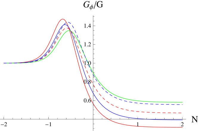
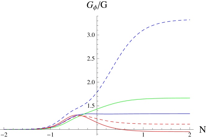
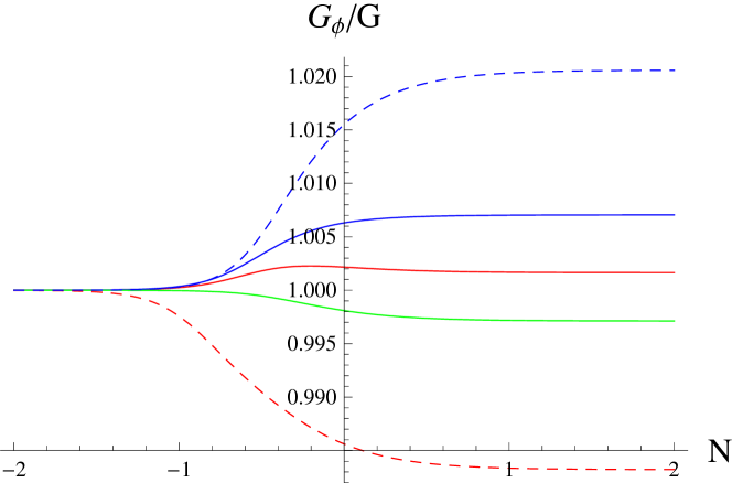
at the dS point (when xdS=1subscript𝑥dS1x_{\rm dS}=1). The limit xdS0subscript𝑥dS0x_{\rm dS}\rightarrow 0 gives us the usual GR result Gϕ(tdS)=Gsubscript𝐺italic-ϕsubscript𝑡dS𝐺G_{\phi}(t_{\rm dS})=G. Instead, the limit xdSsubscript𝑥dSx_{\rm dS}\rightarrow\infty gives Gϕ(tdS)0subscript𝐺italic-ϕsubscript𝑡dS0G_{\phi}(t_{\rm dS})\rightarrow 0, which means, as expected, that the effective gravitational constant becomes small w.r.t. the Newtonian one (GMpl2proportional-to𝐺superscriptsubscript𝑀pl2G\varpropto M_{\rm pl}^{-2}). The plots in Figs. 2, 3 and 4 show that we can vary the asymptotic value of Gϕsubscript𝐺italic-ϕG_{\phi} as we desire, to obtain, in principle, any reasonable model for the late time cosmic acceleration. The difference between the three graphs is the value of the parameter xdSsubscript𝑥dSx_{\rm dS}, which sets the contribution of the Galileon field at the dS point. This result also agrees with the expectations of Eq. (36), quantifying the effective contribution of the scalar field at large distances on observables quantities. Of course, these results do not represent any realistic model, we are only interested here in investigating the range of possibilities offered by the Galileon theory. Moreover, astrophysical and cosmological constraints on the Galileon model have just started being considered [41, 42, 43, 44].
Refer to caption
Figure 2: This plot shows the evolution of Gϕsubscript𝐺italic-ϕG_{\phi}, with xdS=1subscript𝑥dS1x_{\rm dS}=1, in different cases.The values for (α,β)𝛼𝛽(\alpha,\beta) are: (1,0.55)10.55(-1,-0.55), blue dashed line; (0.45,0.4)0.450.4(-0.45,-0.4), red line; (0.2,0.2)0.20.2(-0.2,-0.2), green line; (0.55,0.4)0.550.4(-0.55,-0.4), blue solid line; (0.1,0.1)0.10.1(0.1,-0.1), red dashed line.
Refer to caption
Figure 3: The same as in Fig. 2, but with xdS=0.3subscript𝑥dS0.3x_{\rm dS}=0.3.
Refer to caption
Figure 4: The same as in Fig. 2, but with xdS=1.2subscript𝑥dS1.2x_{\rm dS}=1.2.

4.3 Non-linear evolution

When perturbations grow, Eqs. (27), (28) and (29) must be replaced by fully non-linear ones. Neglecting time-derivatives of perturbations and assuming that the characteristic scale of the perturbation is well within the Hubble radius, we obtain

(2Mpl2+ϕ˙2γ1(t))2Φ=δρ+γ2(t)2φ+γ1(t)[(2φ)2+\displaystyle\left(2M_{\rm pl}^{2}+\dot{\phi}^{2}\gamma_{1}(t)\right)\nabla^{2}\Phi=-\delta\rho+\gamma_{2}(t)\nabla^{2}\varphi+\gamma_{1}(t)\left[{(\nabla^{2}\varphi)}^{2}+\right.
jiφijφ]+η1(t)[(2φ)3+2jiφkjφikφ+\displaystyle\left.-\nabla^{i}_{\phantom{i}j}\varphi\nabla^{j}_{\phantom{j}i}\varphi\right]+\eta_{1}(t)\left[{(\nabla^{2}\varphi)}^{3}+2\nabla^{i}_{\phantom{i}j}\varphi\nabla^{j}_{\phantom{j}k}\varphi\nabla^{k}_{\phantom{k}i}\varphi+\right.
32φjiφijφ]32ϕ˙2η1(t)[2φ2ΦjiΦijφ],\displaystyle\left.-3\nabla^{2}\varphi\nabla^{i}_{\phantom{i}j}\varphi\nabla^{j}_{\phantom{j}i}\varphi\right]-\frac{3}{2}\dot{\phi}^{2}\eta_{1}(t)\left[\nabla^{2}\varphi\nabla^{2}\Phi-\nabla^{i}_{\phantom{i}j}\Phi\nabla^{j}_{\phantom{j}i}\varphi\right]\,, (40)
(2Mpl2+3γ3(t))2Φ+(2Mpl2+ϕ˙2γ1(t))2Ψ=3γ4(t)2φ+2superscriptsubscript𝑀pl23subscript𝛾3𝑡superscript2Φ2superscriptsubscript𝑀pl2superscript˙italic-ϕ2subscript𝛾1𝑡superscript2Ψlimit-from3subscript𝛾4𝑡superscript2𝜑\displaystyle\left(2M_{\rm pl}^{2}+3\gamma_{3}(t)\right)\nabla^{2}\Phi+\left(2M_{\rm pl}^{2}+\dot{\phi}^{2}\gamma_{1}(t)\right)\nabla^{2}\Psi=3\gamma_{4}(t)\nabla^{2}\varphi+
+3η2(t)[(2φ)2jiφijφ]32ϕ˙2η1(t)[2φ2ΨjiΨijφ].3subscript𝜂2𝑡delimited-[]superscriptsuperscript2𝜑2subscriptsuperscript𝑖𝑗𝜑subscriptsuperscript𝑗𝑖𝜑32superscript˙italic-ϕ2subscript𝜂1𝑡delimited-[]superscript2𝜑superscript2Ψsubscriptsuperscript𝑖𝑗Ψsubscriptsuperscript𝑗𝑖𝜑\displaystyle+3\eta_{2}(t)\left[{(\nabla^{2}\varphi)}^{2}-\nabla^{i}_{\phantom{i}j}\varphi\nabla^{j}_{\phantom{j}i}\varphi\right]-\frac{3}{2}\dot{\phi}^{2}\eta_{1}(t)\left[\nabla^{2}\varphi\nabla^{2}\Psi-\nabla^{i}_{\phantom{i}j}\Psi\nabla^{j}_{\phantom{j}i}\varphi\right]\,. (41)

Eq. (29), instead, takes the form

γ5(t)2φ+γ2(t)2Ψ+3γ4(t)2Φ+η3(t)[(2φ)2jiφijφ]subscript𝛾5𝑡superscript2𝜑subscript𝛾2𝑡superscript2Ψ3subscript𝛾4𝑡superscript2Φlimit-fromsubscript𝜂3𝑡delimited-[]superscriptsuperscript2𝜑2subscriptsuperscript𝑖𝑗𝜑subscriptsuperscript𝑗𝑖𝜑\displaystyle\gamma_{5}(t)\nabla^{2}\varphi+\gamma_{2}(t)\nabla^{2}\Psi+3\gamma_{4}(t)\nabla^{2}\Phi+\eta_{3}(t)\left[{(\nabla^{2}\varphi)}^{2}-\nabla^{i}_{\phantom{i}j}\varphi\nabla^{j}_{\phantom{j}i}\varphi\right]-
η4(t)[(2φ)3+2jiφkjφikφ32φjiφijφ]+limit-fromsubscript𝜂4𝑡delimited-[]superscriptsuperscript2𝜑32subscriptsuperscript𝑖𝑗𝜑subscriptsuperscript𝑗𝑘𝜑subscriptsuperscript𝑘𝑖𝜑3superscript2𝜑subscriptsuperscript𝑖𝑗𝜑subscriptsuperscript𝑗𝑖𝜑\displaystyle-\eta_{4}(t)\left[{(\nabla^{2}\varphi)}^{3}+2\nabla^{i}_{\phantom{i}j}\varphi\nabla^{j}_{\phantom{j}k}\varphi\nabla^{k}_{\phantom{k}i}\varphi-3\nabla^{2}\varphi\nabla^{i}_{\phantom{i}j}\varphi\nabla^{j}_{\phantom{j}i}\varphi\right]+
+2γ1(t)[2φ2ΨjiΨijφ]+6η2(t)[2φ2ΦjiΦijφ]2subscript𝛾1𝑡delimited-[]superscript2𝜑superscript2Ψsubscriptsuperscript𝑖𝑗Ψsubscriptsuperscript𝑗𝑖𝜑limit-from6subscript𝜂2𝑡delimited-[]superscript2𝜑superscript2Φsubscriptsuperscript𝑖𝑗Φsubscriptsuperscript𝑗𝑖𝜑\displaystyle+2\gamma_{1}(t)\left[\nabla^{2}\varphi\nabla^{2}\Psi-\nabla^{i}_{\phantom{i}j}\Psi\nabla^{j}_{\phantom{j}i}\varphi\right]+6\eta_{2}(t)\left[\nabla^{2}\varphi\nabla^{2}\Phi-\nabla^{i}_{\phantom{i}j}\Phi\nabla^{j}_{\phantom{j}i}\varphi\right]-
32ϕ˙2η1(t)[2Ψ2ΦjiΦijΨ]+3η1(t)[(2φ)22Ψ\displaystyle-\frac{3}{2}\dot{\phi}^{2}\eta_{1}(t)\left[\nabla^{2}\Psi\nabla^{2}\Phi-\nabla^{i}_{\phantom{i}j}\Phi\nabla^{j}_{\phantom{j}i}\Psi\right]+3\eta_{1}(t)\left[{(\nabla^{2}\varphi)}^{2}\nabla^{2}\Psi-\right.
22φjiφijΨ2Ψjiφijφ+2jiφkjφikΨ]=0,\displaystyle\left.-2\nabla^{2}\varphi\nabla^{i}_{\phantom{i}j}\varphi\nabla^{j}_{\phantom{j}i}\Psi-\nabla^{2}\Psi\nabla^{i}_{\phantom{i}j}\varphi\nabla^{j}_{\phantom{j}i}\varphi+2\nabla^{i}_{\phantom{i}j}\varphi\nabla^{j}_{\phantom{j}k}\varphi\nabla^{k}_{\phantom{k}i}\Psi\right]=0\,, (42)

where the ηi(t)subscript𝜂𝑖𝑡\eta_{i}(t) functions are listed in B.

Eqs. (4.3), (4.3) and (4.3) are more complicated than in the linear case, however, assuming spherical symmetry, they are in fact integrable. The boundary values of the perturbations can be determined by resorting to the physical meaning to these fields. For example, from GR we know that the physical solution of the Poisson equation is

ΨGR(t,r)=Gm(t,r)r2.superscriptsubscriptΨ𝐺𝑅𝑡𝑟𝐺𝑚𝑡𝑟superscript𝑟2{\Psi_{GR}}^{\prime}(t,r)=\frac{Gm(t,r)}{r^{2}}. (43)

Recalling the definition of the mass function, m(t,r)4π0rdrr2δρ(t,r)𝑚𝑡𝑟4𝜋superscriptsubscript0𝑟differential-dsuperscript𝑟superscript𝑟2𝛿𝜌𝑡𝑟m(t,r)\equiv 4\pi\int_{0}^{r}{\rm d}r^{\prime}r^{\prime 2}\delta\rho(t,r), if there are no singularities at r=0𝑟0r=0 for the density perturbation, this relation tells us that ΨGR(t,0)=0superscriptsubscriptΨ𝐺𝑅𝑡00{\Psi_{GR}}^{\prime}(t,0)=0 (to violate this limit we have to choose δρ(r)rnproportional-to𝛿𝜌𝑟superscript𝑟𝑛\delta\rho(r)\propto r^{-n}, with n3𝑛3n\geq 3). At small scales we want to recover GR, so the physical meaning of Ψ(t,r)Ψ𝑡𝑟\Psi(t,r) should be that of gravitational potential (Ψ(t,r)ΨGR(t,r)similar-to-or-equalssuperscriptΨ𝑡𝑟superscriptsubscriptΨ𝐺𝑅𝑡𝑟\Psi^{\prime}(t,r)\simeq{\Psi_{GR}}^{\prime}(t,r)). Indeed, the natural assignment is Ψ(t,0)=0superscriptΨ𝑡00\Psi^{\prime}(t,0)=0. The same argument applies to Φ(t,r0)ΨGR(t,r0)similar-to-or-equalssuperscriptΦ𝑡𝑟0superscriptsubscriptΨ𝐺𝑅𝑡𝑟0\Phi^{\prime}(t,r\rightarrow 0)\simeq-{\Psi_{GR}}^{\prime}(t,r\rightarrow 0). Instead, the scalar field and its perturbations are not directly observable quantities, so we have to choose the correct boundary value by mathematical arguments or by its effect on measurable physical quantities. Like in Eq. (33), at r0𝑟0r\rightarrow 0 there should be some divergent term. However, the same reasoning used in the linear case allows us to consider φ(r0)superscript𝜑𝑟0\varphi^{\prime}(r\rightarrow 0) finite.

Integrating Eqs. (4.3), (4.3) and (4.3) for a spherically symmetric object, we obtain

γ6Φr=m(t,r)4πr3+γ2φr+2γ1φ2r2+2η1φ3r32η1φ(0)3r33ϕ˙2η1φΦr2subscript𝛾6superscriptΦ𝑟𝑚𝑡𝑟4𝜋superscript𝑟3subscript𝛾2superscript𝜑𝑟2subscript𝛾1superscript𝜑2superscript𝑟22subscript𝜂1superscript𝜑3superscript𝑟32subscript𝜂1superscript𝜑superscript03superscript𝑟33superscript˙italic-ϕ2subscript𝜂1superscript𝜑superscriptΦsuperscript𝑟2\gamma_{6}\frac{\Phi^{\prime}}{r}=-\frac{m(t,r)}{4\pi r^{3}}+\gamma_{2}\frac{\varphi^{\prime}}{r}+2\gamma_{1}\frac{\varphi^{\prime 2}}{r^{2}}+2\eta_{1}\frac{\varphi^{\prime 3}}{r^{3}}-2\eta_{1}\frac{{\varphi^{\prime}(0)}^{3}}{r^{3}}-3\dot{\phi}^{2}\eta_{1}\frac{\varphi^{\prime}\Phi^{\prime}}{r^{2}} (44)
γ7Φr+γ6Ψr=3γ4φr+6η2φ2r23ϕ˙2η1φΨr2subscript𝛾7superscriptΦ𝑟subscript𝛾6superscriptΨ𝑟3subscript𝛾4superscript𝜑𝑟6subscript𝜂2superscript𝜑2superscript𝑟23superscript˙italic-ϕ2subscript𝜂1superscript𝜑superscriptΨsuperscript𝑟2\gamma_{7}\frac{\Phi^{\prime}}{r}+\gamma_{6}\frac{\Psi^{\prime}}{r}=3\gamma_{4}\frac{\varphi^{\prime}}{r}+6\eta_{2}\frac{\varphi^{\prime 2}}{r^{2}}-3\dot{\phi}^{2}\eta_{1}\frac{\varphi^{\prime}\Psi^{\prime}}{r^{2}} (45)
γ5φr+γ2Ψr+3γ4Φr+2η3φ2r22η4φ3r3+subscript𝛾5superscript𝜑𝑟subscript𝛾2superscriptΨ𝑟3subscript𝛾4superscriptΦ𝑟2subscript𝜂3superscript𝜑2superscript𝑟2limit-from2subscript𝜂4superscript𝜑3superscript𝑟3\displaystyle\gamma_{5}\frac{\varphi^{\prime}}{r}+\gamma_{2}\frac{\Psi^{\prime}}{r}+3\gamma_{4}\frac{\Phi^{\prime}}{r}+2\eta_{3}\frac{\varphi^{\prime 2}}{r^{2}}-2\eta_{4}\frac{\varphi^{\prime 3}}{r^{3}}+
+2η4φ(0)3r3+4γ1φΨr2+6η1φ2Ψr3+12η2φΦr23ϕ˙2η1ΦΨr22subscript𝜂4superscript𝜑superscript03superscript𝑟34subscript𝛾1superscript𝜑superscriptΨsuperscript𝑟26subscript𝜂1superscript𝜑2superscriptΨsuperscript𝑟312subscript𝜂2superscript𝜑superscriptΦsuperscript𝑟23superscript˙italic-ϕ2subscript𝜂1superscriptΦsuperscriptΨsuperscript𝑟2\displaystyle+2\eta_{4}\frac{{\varphi^{\prime}(0)}^{3}}{r^{3}}+4\gamma_{1}\frac{\varphi^{\prime}\Psi^{\prime}}{r^{2}}+6\eta_{1}\frac{\varphi^{\prime 2}\Psi^{\prime}}{r^{3}}+12\eta_{2}\frac{\varphi^{\prime}\Phi^{\prime}}{r^{2}}-3\dot{\phi}^{2}\eta_{1}\frac{\Phi^{\prime}\Psi^{\prime}}{r^{2}} =\displaystyle= 0,0\displaystyle 0\,, (46)

Note that we have not yet analyzed the case in which the scalar field has a boundary value φ(r=0)superscript𝜑𝑟0\varphi^{\prime}(r=0) finite, but different from zero; to do this we have to impose a physical condition. From Eq. (45), we can write

φ(r)r=γ44η2+ϕ˙2η14η2Ψ(r)r+Sgn(γ4)4η2[(γ4+ϕ˙2η1Ψ(r)r)2+\displaystyle\frac{\varphi^{\prime}(r)}{r}=-\frac{\gamma_{4}}{4\eta_{2}}+\frac{\dot{\phi}^{2}\eta_{1}}{4\eta_{2}}\cdot\frac{\Psi^{\prime}(r)}{r}+\frac{{\rm Sgn}(\gamma_{4})}{4\eta_{2}}\left[{\left(-\gamma_{4}+\dot{\phi}^{2}\eta_{1}\frac{\Psi^{\prime}(r)}{r}\right)}^{2}+\right.
+83η2(2Mpl2+3γ3)Φ(r)r+83η2(2Mpl2+ϕ˙2γ1)Ψ(r)r]1/2;\displaystyle{\left.+\frac{8}{3}\eta_{2}\left(2M_{\rm pl}^{2}+3\gamma_{3}\right)\frac{\Phi^{\prime}(r)}{r}+\frac{8}{3}\eta_{2}\left(2M_{\rm pl}^{2}+\dot{\phi}^{2}\gamma_{1}\right)\frac{\Psi^{\prime}(r)}{r}\right]}^{1/2}\,; (47)

here we have chosen the solution which matches the linear one (33) when r𝑟r\rightarrow\infty.

Without any loss of generality, the metric perturbations can be written as

Ψ(r)=ΨGR(r)[1+δΨ(r)]=Gm(t,r)r2[1+δΨ(r)]superscriptΨ𝑟subscriptsuperscriptΨ𝐺𝑅𝑟delimited-[]1subscript𝛿Ψ𝑟𝐺𝑚𝑡𝑟superscript𝑟2delimited-[]1subscript𝛿Ψ𝑟\displaystyle\Psi^{\prime}(r)=\Psi^{\prime}_{GR}(r)\left[1+\delta_{\Psi}(r)\right]=\frac{G\,m(t,r)}{r^{2}}\left[1+\delta_{\Psi}(r)\right] (48)
Φ(r)=ΦGR(r)[1+δΦ(r)]=Gm(t,r)r2[1+δΦ(r)].superscriptΦ𝑟subscriptsuperscriptΦ𝐺𝑅𝑟delimited-[]1subscript𝛿Φ𝑟𝐺𝑚𝑡𝑟superscript𝑟2delimited-[]1subscript𝛿Φ𝑟\displaystyle\Phi^{\prime}(r)=\Phi^{\prime}_{GR}(r)\left[1+\delta_{\Phi}(r)\right]=-\frac{G\,m(t,r)}{r^{2}}\left[1+\delta_{\Phi}(r)\right]\,. (49)

In this case, ΨGR(r)subscriptΨ𝐺𝑅𝑟\Psi_{GR}(r) can be understood as the gravitational potential generated by a perturbation in the ΛCDMΛCDM\Lambda\textrm{CDM} model. When rrVmuch-less-than𝑟subscript𝑟𝑉r\ll r_{V}, δΨsubscript𝛿Ψ\delta_{\Psi} and δΦsubscript𝛿Φ\delta_{\Phi} have to be small by solar-system constraints (δΨ,δΦ103less-than-or-similar-tosubscript𝛿Ψsubscript𝛿Φsuperscript103\delta_{\Psi}\,,\delta_{\Phi}\lesssim 10^{-3}), so we can treat them as small perturbations. In this limit, at first order, Eq. (4.3) becomes

φ(r)rsuperscript𝜑𝑟𝑟\displaystyle\frac{\varphi^{\prime}(r)}{r} similar-to-or-equals\displaystyle\simeq γ44η2+ϕ˙2η1ΨGR(r)4η2r+Sgn(γ4)f(t,r)4η2+ϕ˙2η1ΨGR(r)4η2rδΨ(t,r)+subscript𝛾44subscript𝜂2superscript˙italic-ϕ2subscript𝜂1subscriptsuperscriptΨ𝐺𝑅𝑟4subscript𝜂2𝑟Sgnsubscript𝛾4𝑓𝑡𝑟4subscript𝜂2limit-fromsuperscript˙italic-ϕ2subscript𝜂1subscriptsuperscriptΨ𝐺𝑅𝑟4subscript𝜂2𝑟subscript𝛿Ψ𝑡𝑟\displaystyle-\frac{\gamma_{4}}{4\eta_{2}}+\frac{\dot{\phi}^{2}\eta_{1}\Psi^{\prime}_{GR}(r)}{4\eta_{2}r}+\frac{{\rm Sgn}(\gamma_{4})f(t,r)}{4\eta_{2}}+\frac{\dot{\phi}^{2}\eta_{1}\Psi^{\prime}_{GR}(r)}{4\eta_{2}r}\delta_{\Psi}(t,r)+ (50)
+Sgn(γ4)ΨGR(r)12η2f(t,r)r[3ϕ˙4η12ΨGR(r)r3ϕ˙2γ4η1+4γ6η2]δΨ(t,r)+limit-fromSgnsubscript𝛾4subscriptsuperscriptΨ𝐺𝑅𝑟12subscript𝜂2𝑓𝑡𝑟𝑟delimited-[]3superscript˙italic-ϕ4superscriptsubscript𝜂12subscriptsuperscriptΨ𝐺𝑅𝑟𝑟3superscript˙italic-ϕ2subscript𝛾4subscript𝜂14subscript𝛾6subscript𝜂2subscript𝛿Ψ𝑡𝑟\displaystyle+\frac{{\rm Sgn}(\gamma_{4})\Psi^{\prime}_{GR}(r)}{12\eta_{2}f(t,r)r}\left[3\dot{\phi}^{4}{\eta_{1}}^{2}\frac{\Psi^{\prime}_{GR}(r)}{r}-3\dot{\phi}^{2}\gamma_{4}\eta_{1}+4\gamma_{6}\eta_{2}\right]\delta_{\Psi}(t,r)+
Sgn(γ4)γ7ΨGR(r)f(t,r)rδΦ(t,r),Sgnsubscript𝛾4subscript𝛾7subscriptsuperscriptΨ𝐺𝑅𝑟𝑓𝑡𝑟𝑟subscript𝛿Φ𝑡𝑟\displaystyle-\frac{{\rm Sgn}(\gamma_{4})\gamma_{7}\Psi^{\prime}_{GR}(r)}{f(t,r)r}\delta_{\Phi}(t,r)\,,

where

f(t,r)𝑓𝑡𝑟\displaystyle f(t,r) \displaystyle\equiv [γ42+ϕ˙4η12ΨGR(r)2r28γ3η2ΨGR(r)r2ϕ˙2γ4η1ΨGR(r)r+\displaystyle\left[{\gamma_{4}}^{2}+\dot{\phi}^{4}{\eta_{1}}^{2}\frac{{\Psi^{\prime}_{GR}(r)}^{2}}{r^{2}}-8\gamma_{3}\eta_{2}\frac{\Psi^{\prime}_{GR}(r)}{r}-2\dot{\phi}^{2}\gamma_{4}\eta_{1}\frac{\Psi^{\prime}_{GR}(r)}{r}+\right. (51)
+83ϕ˙2γ1η2ΨGR(r)r]1/2.\displaystyle{\left.+\frac{8}{3}\dot{\phi}^{2}\gamma_{1}\eta_{2}\frac{\Psi^{\prime}_{GR}(r)}{r}\right]}^{1/2}\,.

From Eq. (50), we are now ready to choose a reasonable boundary value for φ(r)superscript𝜑𝑟\varphi^{\prime}(r). It is sufficient to suppose that neither δΨsubscript𝛿Ψ\delta_{\Psi} nor δΦsubscript𝛿Φ\delta_{\Phi} diverge in the limit r0𝑟0r\rightarrow 0, to show that φ(r0)=0superscript𝜑𝑟00\varphi^{\prime}(r\rightarrow 0)=0.

4.4 Vainshtein radius

Having obtained the non-linear equations of motion, we are now ready to investigate the radius at which non-linearities become important. The simplest way to estimate rVsubscript𝑟𝑉r_{V} is to plug-in the linear solutions into the non-linear equations, and estimate when the non-linear terms become comparable with the linear ones. First, considering Eq. (44), from the quadratic term we obtain

2γ1γ2φr|r=rV11.similar-to-or-equalsevaluated-at2subscript𝛾1subscript𝛾2superscript𝜑𝑟𝑟subscript𝑟subscript𝑉11\left.2\frac{\gamma_{1}}{\gamma_{2}}\cdot\frac{\varphi^{\prime}}{r}\right|_{r=r_{V_{1}}}\simeq 1\,. (52)

To solve this equation, we need to know the matter density profile. However, using Eq. (33), in the general case we find

rV13=γ1(t)A(t)2πγ2(t)[m(t,r)+Δm(t,r,rV1)],superscriptsubscript𝑟subscript𝑉13subscript𝛾1𝑡𝐴𝑡2𝜋subscript𝛾2𝑡delimited-[]𝑚𝑡𝑟Δ𝑚𝑡𝑟subscript𝑟subscript𝑉1{r_{V_{1}}}^{3}=\frac{\gamma_{1}(t)A(t)}{2\pi\gamma_{2}(t)}\left[m(t,r)+\Delta m(t,r,r_{V_{1}})\right]\,, (53)

where Δm(t,r,rV1)=4πrrV1𝑑rr2δρΔ𝑚𝑡𝑟subscript𝑟subscript𝑉14𝜋superscriptsubscript𝑟subscript𝑟subscript𝑉1differential-dsuperscript𝑟superscriptsuperscript𝑟2𝛿𝜌\Delta m(t,r,r_{V_{1}})=4\pi\int_{r}^{r_{V_{1}}}dr^{\prime}{r^{\prime}}^{2}\delta\rho. The interior solution for a top-hat profile leads to an r𝑟r-invariant equation. The simple consideration is that, depending on the epoch and on the choice of the background parameters, we can have this region all inside or all outside the Vainshtein region. Instead, outside a source of mass Mssubscript𝑀𝑠M_{s} we find (defining RVrV(R)subscript𝑅𝑉subscript𝑟𝑉𝑅R_{V}\equiv r_{V}(R))

(RV1R)3=|2γ1γ2A(t)Ms4πR3|.superscriptsubscript𝑅subscript𝑉1𝑅32subscript𝛾1subscript𝛾2𝐴𝑡subscript𝑀𝑠4𝜋superscript𝑅3{\left(\frac{{R_{V_{1}}}}{R}\right)}^{3}=\left|\frac{2\gamma_{1}}{\gamma_{2}}\cdot\frac{A(t)M_{s}}{4\pi R^{3}}\right|\,. (54)

The same procedure for the cubic term leads to

(RV2R)3=|2η1γ2A(t)Ms4πR3|.superscriptsubscript𝑅subscript𝑉2𝑅32subscript𝜂1subscript𝛾2𝐴𝑡subscript𝑀𝑠4𝜋superscript𝑅3{\left(\frac{R_{V_{2}}}{R}\right)}^{3}=\left|\sqrt{\frac{2\eta_{1}}{\gamma_{2}}}\cdot\frac{A(t)M_{s}}{4\pi R^{3}}\right|\,. (55)

Comparing the two Vainshtein radii we see that they are comparable. This means that we have an exterior linear region, but, when we enter the non-linear one, quadratic and cubic terms can both dominate. Indeed, the contribution derived from the terms c4subscript𝑐4c_{4} and c5subscript𝑐5c_{5} influences in a non-negligible way the scalar field profile. This also proves that at sufficiently large distances we recover the predictions of the linear theory, discussed in Sec. 4.1.

Other three important Vainshtein radii, coming from Eqs. (45) and (4.3), are

(RV3R)3=2η2γ4A(t)Ms4πR3,superscriptsubscript𝑅subscript𝑉3𝑅32subscript𝜂2subscript𝛾4𝐴𝑡subscript𝑀𝑠4𝜋superscript𝑅3{\left(\frac{{R_{V_{3}}}}{R}\right)}^{3}=\frac{2\eta_{2}}{\gamma_{4}}\cdot\frac{A(t)M_{s}}{4\pi R^{3}}\,, (56)
(RV4R)3=2η3γ5A(t)Ms4πR3.superscriptsubscript𝑅subscript𝑉4𝑅32subscript𝜂3subscript𝛾5𝐴𝑡subscript𝑀𝑠4𝜋superscript𝑅3{\left(\frac{{R_{V_{4}}}}{R}\right)}^{3}=\frac{2\eta_{3}}{\gamma_{5}}\cdot\frac{A(t)M_{s}}{4\pi R^{3}}\,. (57)

and:

(RV5R)3=2η4γ5A(t)Ms4πR3.superscriptsubscript𝑅subscript𝑉5𝑅32subscript𝜂4subscript𝛾5𝐴𝑡subscript𝑀𝑠4𝜋superscript𝑅3{\left(\frac{{R_{V_{5}}}}{R}\right)}^{3}=\sqrt{\frac{2\eta_{4}}{\gamma_{5}}}\cdot\frac{A(t)M_{s}}{4\pi R^{3}}\,. (58)

Here we have neglected non-linear interactions which couple φ𝜑\varphi with ΦΦ\Phi and ΨΨ\Psi, because they produce results analogous to the previous ones. The Vainshtein radius can be set as RVMax(RVi)subscript𝑅𝑉Maxsubscript𝑅subscript𝑉𝑖R_{V}\equiv{\rm Max}(R_{V_{i}}), where i=1,..,11i=1,..,11. It is straightforward to prove that RV(t)+subscript𝑅𝑉𝑡R_{V}(t\rightarrow-\infty)\rightarrow+\infty, while RV(t+)=f(α,β,xdS)Ms/(4πMplHdS2)subscript𝑅𝑉𝑡𝑓𝛼𝛽subscript𝑥dSsubscript𝑀𝑠4𝜋subscript𝑀plsuperscriptsubscript𝐻dS2R_{V}(t\rightarrow+\infty)=f(\alpha,\beta,x_{\rm dS})M_{s}/(4\pi M_{\rm pl}H_{\rm dS}^{2}), where f𝑓f is a generic function of the background parameters. This result agrees with the predictions of [35] and [36].

4.5 Galileon field evolution

In this section we study the Galileon field evolution, starting from Eqs. (44), (45) and (4.3). These are three algebraic equations in Ψ(r)superscriptΨ𝑟\Psi^{\prime}(r), Φ(r)superscriptΦ𝑟\Phi^{\prime}(r) and φ(r)superscript𝜑𝑟\varphi^{\prime}(r), so it is straightforward to obtain a sixth-order polynomial equation in φ(r)superscript𝜑𝑟\varphi^{\prime}(r) (to simplify the problem we will work under the assumption that xds=1subscript𝑥ds1x_{\rm ds}=1):

φ6r6+λ1(t)φ5r5+λ2(t)φ4r4+(λ3(t)δm+λ4(t))φ3r3+(λ5(t)δm+\displaystyle\frac{\varphi^{\prime 6}}{r^{6}}+\lambda_{1}(t)\frac{\varphi^{\prime 5}}{r^{5}}+\lambda_{2}(t)\frac{\varphi^{\prime 4}}{r^{4}}+\left(\lambda_{3}(t)\delta_{m}+\lambda_{4}(t)\right)\frac{\varphi^{\prime 3}}{r^{3}}+\left(\lambda_{5}(t)\delta_{m}+\right.
+λ6(t))φ2r2+(λ7(t)δm+λ8(t))φr+λ9(t)δm+λ10(t)δm2=0,\displaystyle\left.+\lambda_{6}(t)\right)\frac{\varphi^{\prime 2}}{r^{2}}+\left(\lambda_{7}(t)\delta_{m}+\lambda_{8}(t)\right)\frac{\varphi^{\prime}}{r}+\lambda_{9}(t)\delta_{m}+\lambda_{10}(t){\delta_{m}}^{2}=0\,, (59)

where λisubscript𝜆𝑖\lambda_{i} are background functions, combinations of γisubscript𝛾𝑖\gamma_{i} and ηisubscript𝜂𝑖\eta_{i}. From Eq. (4.5) it follows that φ(r)superscript𝜑𝑟\varphi^{\prime}(r) has six branches of solutions. What is the correct one? Remembering the Vainshtein effect, we want that the physical solution reduces to Eq. (33) at large distances. Of course, this condition cannot be verified analytically, but it is sufficient to choose between the real solutions of Eq. (4.5).

Are we sure that, for a given couple (α,β)𝛼𝛽(\alpha,\beta), Eq. (4.5) has at least a couple of solutions during the whole evolution of the universe? Obviously this condition is not sufficient to ensure the existence of the physical solution, but it is a necessary condition. In the linear regime the existence of a physical solution was proved in Sec. 4.1, thus the problems can be inside the Vainshtein radius. As proved in Sec. 4.4, at small distances non-linear terms become dominant for the evolution of the scalar field. In particular, instead of Eq. (4.5), we can work with the equation

φ6r6+λ1(t)φ5r5+λ2(t)φ4r4+λ10(t)δm2=0.superscript𝜑6superscript𝑟6subscript𝜆1𝑡superscript𝜑5superscript𝑟5subscript𝜆2𝑡superscript𝜑4superscript𝑟4subscript𝜆10𝑡superscriptsubscript𝛿𝑚20\frac{\varphi^{\prime 6}}{r^{6}}+\lambda_{1}(t)\frac{\varphi^{\prime 5}}{r^{5}}+\lambda_{2}(t)\frac{\varphi^{\prime 4}}{r^{4}}+\lambda_{10}(t){\delta_{m}}^{2}=0. (60)

Also in this case we do not have an analytic solution for the scalar field; however Eq. (60) gives new constraints on the allowed region in the parameter space (α,β)𝛼𝛽(\alpha,\beta).

Consider a function like

f(x)=x6+Ax5+Bx4+C,𝑓𝑥superscript𝑥6𝐴superscript𝑥5𝐵superscript𝑥4𝐶f(x)=x^{6}+A\,x^{5}+B\,x^{4}+C\,, (61)

where A,B,C0𝐴𝐵𝐶0A,\,B,\,C\neq 0 are real coefficients. The RHS of this equation has the same form as Eq. (60), after the substitution φ(t,r)/rxsuperscript𝜑𝑡𝑟𝑟𝑥\varphi^{\prime}(t,r)/r\rightarrow x. It was demonstrated that there is no analytic method to find a solution for f(x)=0𝑓𝑥0f(x)=0, when f(x)𝑓𝑥f(x) is a fifth or higher degree polynomial. However, since

limx±f(x)=+,subscript𝑥plus-or-minus𝑓𝑥\lim_{x\to\pm\infty}f(x)=+\infty\,, (62)

it is sufficient to require that a minimum of this function is <0absent0<0, to be sure to have at least a couple of real solutions. The points which satisfy f(x)=0superscript𝑓𝑥0f^{\prime}(x)=0 are

x1,2,3=0x4,5=512A±25144A223B.formulae-sequencesubscript𝑥1230subscript𝑥45plus-or-minus512𝐴25144superscript𝐴223𝐵x_{1,2,3}=0\qquad x_{4,5}=-\frac{5}{12}A\pm\sqrt{\frac{25}{144}A^{2}-\frac{2}{3}B}\,. (63)

The zeros of Eq. (4.5) can be understood as six perturbative terms around xisubscript𝑥𝑖x_{i}. Let us assume that, for the purpose of this section, these perturbations are small. The set of parameters for which f(x)=0𝑓𝑥0f(x)=0 has at least a couple of solutions, which are given by

f(x1)<0f(x4)<0f(x5)<0.formulae-sequence𝑓subscript𝑥10formulae-sequence𝑓subscript𝑥40𝑓subscript𝑥50f(x_{1})<0\quad\vee\quad f(x_{4})<0\quad\vee\quad f(x_{5})<0\,. (64)

Substituting our background functions into the parameters A,B,C𝐴𝐵𝐶A,\,B,\,C, we must pay attention to the dependence on t𝑡t, because the previous inequalities have to be hold true tfor-all𝑡\forall\,t. The first one becomes

f(x1)=Hds12MPl6144ϕ˙4β2(ϕ˙HdsMPl)4[α+6β(ϕ¨Hds2MPl)]24+(ϕ˙HdsMPl)4[5α+42β(ϕ¨Hds2MPl)]δm(t)2<0.𝑓subscript𝑥1superscriptsubscript𝐻ds12superscriptsubscript𝑀Pl6144superscript˙italic-ϕ4superscript𝛽2superscript˙italic-ϕsubscript𝐻dssubscript𝑀Pl4delimited-[]𝛼6𝛽¨italic-ϕsuperscriptsubscript𝐻ds2subscript𝑀Pl24superscript˙italic-ϕsubscript𝐻dssubscript𝑀Pl4delimited-[]5𝛼42𝛽¨italic-ϕsuperscriptsubscript𝐻ds2subscript𝑀Plsubscript𝛿𝑚superscript𝑡20f(x_{1})=\frac{H_{\rm ds}^{12}\,M_{\rm Pl}^{6}}{144\,\dot{\phi}^{4}\,\beta^{2}}\cdot\frac{\left(\frac{\dot{\phi}}{H_{\rm ds}M_{\rm Pl}}\right)^{4}\left[\alpha+6\beta\left(\frac{\ddot{\phi}}{H_{\rm ds}^{2}M_{\rm Pl}}\right)\right]-2}{4+\left(\frac{\dot{\phi}}{H_{\rm ds}M_{\rm Pl}}\right)^{4}\left[-5\alpha+42\beta\left(\frac{\ddot{\phi}}{H_{\rm ds}^{2}M_{\rm Pl}}\right)\right]}\delta_{m}(t)^{2}<0\,. (65)

It can be proved that this condition is verified tfor-all𝑡\forall\,t, when

{α<4/5α5.22β+1.93α3.73β+4.83.cases𝛼45less-than-or-similar-to𝛼5.22𝛽1.93less-than-or-similar-to𝛼3.73𝛽4.83\left\{\begin{array}[]{l}\alpha<4/5\\ \alpha\lesssim 5.22\beta+1.93\\ \alpha\lesssim-3.73\beta+4.83\,.\end{array}\right. (66)

These relations were obtained evaluating the above expression at some critical times, when f(x1)𝑓subscript𝑥1f(x_{1}) results maximized/minimized. We were able to do this because f(0)𝑓0f(0) takes a simple form, but this is not the case for f(x4)𝑓subscript𝑥4f(x_{4}) and f(x5)𝑓subscript𝑥5f(x_{5}). In fact, the form of these functions at the points x4,5subscript𝑥45x_{4,5} is

f(x4,5)𝑓subscript𝑥45\displaystyle f(x_{4,5}) =\displaystyle= C2126(±5A+25A296B)4(5A224B+\displaystyle C-\frac{2}{12^{6}}{\left(\pm 5A+\sqrt{25A^{2}-96B}\right)}^{4}\left(5A^{2}-24B+\right. (67)
±A25A296B).\displaystyle\left.\pm A\sqrt{25A^{2}-96B}\right)\,.

In our case, the parameter C𝐶C depends on the matter-density perturbation, so the inequalities which follow from the above expression have to be evaluated in two distinct cases. The first one is when the density term dominates on the other terms (the analysis is the same as in f(0)<0𝑓00f(0)<0 case), the second one when it is subdominant. The latter case involves more complicated expressions for the parameters α𝛼\alpha and β𝛽\beta, so we were only able to solve it numerically. Combining these results with the no-ghost condition given in [30], the constraints on the parameters α𝛼\alpha and β𝛽\beta become

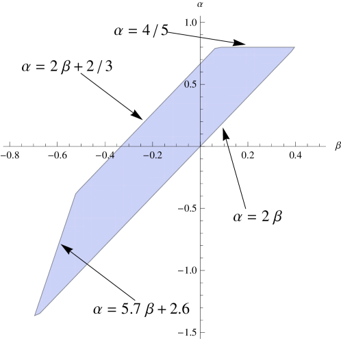
{α>2βα<2β+2/3α<4/5α5.7β+2.62,cases𝛼2𝛽𝛼2𝛽23𝛼45less-than-or-similar-to𝛼5.7𝛽2.62\left\{\begin{array}[]{l}\alpha>2\,\beta\\ \alpha<2\,\beta+2/3\\ \alpha<4/5\\ \alpha\lesssim 5.7\,\beta+2.62\,,\end{array}\right. (68)

and are represented in Fig. 5.

Refer to caption
Figure 5: In this figure we show the allowed region in the plane (β,α)𝛽𝛼(\beta,\alpha) obtained by mixing the no-ghost conditions and the conditions for the existence of the scalar field in the non-linear regime.

5 Spherical Collapse

In this section we will restrict our analysis to a top-hat matter configuration

ρ(r)={ρ0+δρrRρ0r>R,m(r)={δM(r/R)3rRδMr>R.formulae-sequence𝜌𝑟casessubscript𝜌0𝛿𝜌𝑟𝑅subscript𝜌0𝑟𝑅𝑚𝑟cases𝛿𝑀superscript𝑟𝑅3𝑟𝑅𝛿𝑀𝑟𝑅\displaystyle\rho(r)=\left\{\begin{array}[]{ll}\rho_{0}+\delta\rho&~{}~{}~{}~{}r\leq R\\ \rho_{0}&~{}~{}~{}~{}r>R\\ \end{array}\right.,\hskip 2.84544ptm(r)=\left\{\begin{array}[]{ll}\delta M\,(r/R)^{3}&~{}~{}~{}~{}r\leq R\\ \delta M&~{}~{}~{}~{}r>R\\ \end{array}\right.. (73)

The mass δM𝛿𝑀\delta M is the total mass of the density perturbation δρ𝛿𝜌\delta\rho, while M4/3π(ρ0+δρ)R3𝑀43𝜋subscript𝜌0𝛿𝜌superscript𝑅3M\equiv 4/3\,\pi\,(\rho_{0}+\delta\rho)\,R^{3}. The two masses are related by

δM=δ1+δM,𝛿𝑀𝛿1𝛿𝑀\delta M=\frac{\delta}{1+\delta}\,M\,, (74)

where δδρ/ρ0𝛿𝛿𝜌subscript𝜌0\delta\equiv\delta\rho/\rho_{0} is the density contrast.

To study the dynamics of a spherical matter perturbation we need the well known equation

δ¨43δ˙21+δ+2Hδ˙=(1+δ)2Ψ,¨𝛿43superscript˙𝛿21𝛿2𝐻˙𝛿1𝛿superscript2Ψ\ddot{\delta}-\frac{4}{3}\frac{{\dot{\delta}}^{2}}{1+\delta}+2H\dot{\delta}=(1+\delta)\,\nabla^{2}\Psi\,, (75)

which follows from the non-linear continuity and the Euler equation for a pressureless fluid of non-relativistic matter in a top-hat configuration [34]. Eqs. (4.3), (4.3) and (4.3) tell us that, inside a top-hat density perturbation, Ψ(r)rproportional-tosuperscriptΨ𝑟𝑟\Psi^{\prime}(r)\propto r, which means that 2Ψsuperscript2Ψ\nabla^{2}\Psi will be r𝑟r-independent. Indeed, a top-hat profile, remains a top-hat profile during its whole evolution despite the non-validity of Birkhoff’s theorem.

To solve Eq. (75), we have followed [34]; here we briefly summarize the main steps. Assuming the total mass conservation, R3ρ0(1+δ)=const.superscript𝑅3subscript𝜌01𝛿constR^{3}\,\rho_{0}\,(1+\delta)={\rm const.}, Eq. (75) can be rewritten in terms of R

R¨R=H2+H˙132Ψ.¨𝑅𝑅superscript𝐻2˙𝐻13superscript2Ψ\frac{\ddot{R}}{R}\,=\,H^{2}+\dot{H}-\frac{1}{3}\nabla^{2}\Psi\,. (76)

From this equation we can distinguish all the sources that affect the collapse dynamics: H2+H˙superscript𝐻2˙𝐻H^{2}+\dot{H} contains the contribution of the background (matter and dark energy), while 2Ψsuperscript2Ψ\nabla^{2}\Psi contains the contribution of matter and scalar field perturbations. Using N=lna𝑁𝑎N=\ln a as a time variable and defining

yRRiaai,𝑦𝑅subscript𝑅𝑖𝑎subscript𝑎𝑖y\equiv\frac{R}{R_{i}}-\frac{a}{a_{i}}\,, (77)

where Risubscript𝑅𝑖R_{i} and aisubscript𝑎𝑖a_{i} are the initial radius of the perturbation and the initial scale factor, Eq. (76) becomes

y′′+HHy(1+HH)y=13(y+eNNi)2Ψ,superscript𝑦′′superscript𝐻𝐻superscript𝑦1superscript𝐻𝐻𝑦13𝑦superscript𝑒𝑁subscript𝑁𝑖superscript2Ψy^{\prime\prime}+\frac{H^{\prime}}{H}\,y^{\prime}-\left(1+\frac{H^{\prime}}{H}\right)\,y=-\frac{1}{3}\,\left(y+e^{N-N_{i}}\right)\,\nabla^{2}\Psi\,, (78)

where a prime denotes differentiation w.r.t. N𝑁N. The density contrast is

δ=(1+δi)(eNiNy+1)31.𝛿1subscript𝛿𝑖superscriptsuperscript𝑒subscript𝑁𝑖𝑁𝑦131\delta=\left(1+\delta_{i}\right)\cdot{\left(e^{N_{i}-N}y+1\right)}^{-3}-1\,. (79)

Eq. (78) can be solved numerically setting the initial conditions. From Eq. (77) we know that yi=0subscript𝑦𝑖0y_{i}=0 and yi=δi/(3(1+δi))subscriptsuperscript𝑦𝑖subscriptsuperscript𝛿𝑖31subscript𝛿𝑖y^{\prime}_{i}=-\delta^{\prime}_{i}/(3(1+\delta_{i})). Supposing that the perturbations start growing linearly during matter-dominance, the linearization of Eq. (75) can be solved analytically. The growing mode is δaproportional-to𝛿𝑎\delta\propto a, so δ=δsuperscript𝛿𝛿\delta^{\prime}=\delta, thus the second initial condition becomes yi=δi/3subscriptsuperscript𝑦𝑖subscript𝛿𝑖3y^{\prime}_{i}=-\delta_{i}/3. We also set ai=105subscript𝑎𝑖superscript105a_{i}=10^{-5}, while the initial density perturbation is set to collapse exactly at a0=1subscript𝑎01a_{0}=1.

5.1 Virialisation

The Virial Theorem states that a stable system must satisfy the relation

W+2T=0,𝑊2𝑇0W+2T=0\,, (80)

where

T12d3xρv2=310MR˙2𝑇12superscript𝑑3𝑥𝜌superscript𝑣2310𝑀superscript˙𝑅2T\equiv\frac{1}{2}\int d^{3}x\rho v^{2}=\frac{3}{10}M\dot{R}^{2} (81)

is the kinetic energy (the last equality holds true for a top-hat profile), while

Wd3xρm(x)xΨ=3MR3i0Rdrr3dΨi(r)dr𝑊superscript𝑑3𝑥subscript𝜌𝑚𝑥𝑥Ψ3𝑀superscript𝑅3subscript𝑖superscriptsubscript0𝑅differential-d𝑟superscript𝑟3dsubscriptΨ𝑖𝑟d𝑟W\equiv-\int d^{3}x\rho_{m}(\vec{x})\vec{x}\cdot\nabla\Psi=-\frac{3M}{R^{3}}\sum_{i}\int_{0}^{R}{\rm d}r\cdot r^{3}\frac{{\rm d}\Psi_{i}(r)}{{\rm d}r} (82)

is the trace of the potential energy tensor. As in the previous equation the last equality holds true only for a top-hat profile. Ψi(r)subscriptΨ𝑖𝑟\Psi_{i}(r) denotes each component that contributes to the total gravitational potential.

Usually energy conservation is used, but, as noted in [35], for a time-dependent dark energy model, energy is not strictly conserved. So, during the collapse phase, the virial radius can be estimated as the radius at which the virial condition (80) is satisfied.

Important quantities that can be extrapolated from the dynamics of the collapse are the linearized density contrast δcsubscript𝛿𝑐\delta_{c}, and the virial overdensity:

Δvirρvirρcollapse=[1+δ(Rvir)](acollapseavir)3.subscriptΔ𝑣𝑖𝑟subscript𝜌𝑣𝑖𝑟subscript𝜌𝑐𝑜𝑙𝑙𝑎𝑝𝑠𝑒delimited-[]1𝛿subscript𝑅𝑣𝑖𝑟superscriptsubscript𝑎𝑐𝑜𝑙𝑙𝑎𝑝𝑠𝑒subscript𝑎𝑣𝑖𝑟3\Delta_{vir}\equiv\frac{\rho_{vir}}{\rho_{collapse}}=\left[1+\delta(R_{vir})\right]\cdot{\left(\frac{a_{collapse}}{a_{vir}}\right)}^{3}\,. (83)

5.2 Numerical Results

5.2.1 Case β=0𝛽0\beta=0, xdS=1subscript𝑥dS1x_{\rm dS}=1.

This is the case in which the fifth term of Eq. (2) gives no contribution. Eqs. (44), (45) and (4.3) become simpler. In particular, the modified Poisson equation reads

2Ψsuperscript2Ψ\displaystyle\nabla^{2}\Psi =\displaystyle= 3ΩmHdS2a3x42x4α2x4+3αδ+limit-from3subscriptΩ𝑚superscriptsubscript𝐻dS2superscript𝑎3superscript𝑥42superscript𝑥4𝛼2superscript𝑥43𝛼𝛿\displaystyle 3\Omega_{m}H_{\rm dS}^{2}a^{-3}x^{4}\frac{2x^{4}-\alpha}{2x^{4}+3\alpha}\,\delta+ (84)
3HdS2x2[2x4(2+α)+α(2+15α)]36α(2x4+3α)H˙HdS2Mpl(2x4+3α)2φr+limit-from3superscriptsubscript𝐻dS2superscript𝑥2delimited-[]2superscript𝑥42𝛼𝛼215𝛼36𝛼2superscript𝑥43𝛼˙𝐻superscriptsubscript𝐻dS2subscript𝑀plsuperscript2superscript𝑥43𝛼2superscript𝜑𝑟\displaystyle-\frac{3H_{\rm dS}^{2}x^{2}\left[2x^{4}(2+\alpha)+\alpha(-2+15\alpha)\right]-36\alpha(2x^{4}+3\alpha)\dot{H}}{H_{\rm dS}^{2}M_{\rm pl}{(2x^{4}+3\alpha)}^{2}}\cdot\frac{\varphi^{\prime}}{r}+
12αx2(2x43α)HdS2Mpl2(2x4+3α)2φ2r2,12𝛼superscript𝑥22superscript𝑥43𝛼superscriptsubscript𝐻dS2superscriptsubscript𝑀pl2superscript2superscript𝑥43𝛼2superscript𝜑2superscript𝑟2\displaystyle-\frac{12\alpha x^{2}(2x^{4}-3\alpha)}{H_{\rm dS}^{2}M_{\rm pl}^{2}{(2x^{4}+3\alpha)}^{2}}\cdot\frac{\varphi^{\prime 2}}{r^{2}}\,,

with xH/HdS𝑥𝐻subscript𝐻dSx\equiv H/H_{\rm dS}, and φsuperscript𝜑\varphi^{\prime} is a solution of:

α1φ3r3+α2φ2r2+(α3+α4δ)φr+α5δ=0,subscript𝛼1superscript𝜑3superscript𝑟3subscript𝛼2superscript𝜑2superscript𝑟2subscript𝛼3subscript𝛼4𝛿superscript𝜑𝑟subscript𝛼5𝛿0\alpha_{1}\cdot\frac{\varphi^{\prime 3}}{r^{3}}+\alpha_{2}\cdot\frac{\varphi^{\prime 2}}{r^{2}}+\left(\alpha_{3}+\alpha_{4}\delta\right)\cdot\frac{\varphi^{\prime}}{r}+\alpha_{5}\delta=0\,, (85)

with:

α1subscript𝛼1\displaystyle\alpha_{1} =\displaystyle= 4αx2(4x8+24x4α45α2)4𝛼superscript𝑥24superscript𝑥824superscript𝑥4𝛼45superscript𝛼2\displaystyle 4\alpha x^{2}\left(4x^{8}+24x^{4}\alpha-45\alpha^{2}\right) (86)
α2subscript𝛼2\displaystyle\alpha_{2} =\displaystyle= 2Mpl[HdS2x2(4x4(2+3α)(x4+6α)9α2(221α))+\displaystyle 2M_{\rm pl}\left[H_{\rm dS}^{2}x^{2}\left(4x^{4}(2+3\alpha)(x^{4}+6\alpha)-9\alpha^{2}(2-21\alpha)\right)+\right. (87)
+6α(4x824αx445α2)H˙]\displaystyle\left.+6\alpha\left(4x^{8}-24\alpha x^{4}-45\alpha^{2}\right)\dot{H}\right]
α3subscript𝛼3\displaystyle\alpha_{3} =\displaystyle= 2HdS2Mpl2[HdS2x2[2x8(2+α)+x4(4+8α+21α2)+\displaystyle-2H_{\rm dS}^{2}M_{\rm pl}^{2}\left[H_{\rm dS}^{2}x^{2}\left[2x^{8}(2+\alpha)+x^{4}\left(-4+8\alpha+21\alpha^{2}\right)+\right.\right.
+α(221α+45α2)][4x8(2+3α)+27α2(2+5α)+\displaystyle\left.\left.+\alpha\left(2-21\alpha+45\alpha^{2}\right)\right]-\left[4x^{8}(2+3\alpha)+27\alpha^{2}(-2+5\alpha)+\right.\right.
+12x4α(2+9α)]H˙]\displaystyle\left.\left.+12x^{4}\alpha(-2+9\alpha)\right]\dot{H}\right] (88)
α4subscript𝛼4\displaystyle\alpha_{4} =\displaystyle= 8e3nHdS4Mpl2Ωmx4(2x43α)α8superscript𝑒3𝑛superscriptsubscript𝐻dS4superscriptsubscript𝑀pl2subscriptΩ𝑚superscript𝑥42superscript𝑥43𝛼𝛼\displaystyle-8e^{-3n}H_{\rm dS}^{4}M_{\rm pl}^{2}\Omega_{m}x^{4}\left(2x^{4}-3\alpha\right)\alpha (89)
α5subscript𝛼5\displaystyle\alpha_{5} =\displaystyle= e3nHdS4Mpl3Ωmx2[HdS2x2(2x4(2+α)+α(2+15α))+\displaystyle-e^{-3n}H_{\rm dS}^{4}M_{\rm pl}^{3}\Omega_{m}x^{2}\left[H_{\rm dS}^{2}x^{2}\left(2x^{4}(2+\alpha)+\alpha(-2+15\alpha)\right)+\right.
12α(2x4+3α)H˙].\displaystyle\left.-12\alpha\left(2x^{4}+3\alpha\right)\dot{H}\right]\,. (90)

Of course, among the solutions we want the one that reduces to Eq. (33) when rrVmuch-greater-than𝑟subscript𝑟𝑉r\gg r_{V}.

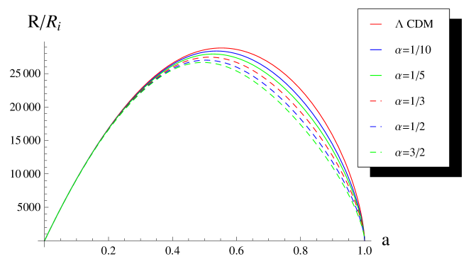
Although this is a particular case, it is interesting to show the role of 4subscript4{\cal L}_{4} in Eq. (2). In Fig. 6 we have plotted the solution of Eq. (78) for various α𝛼\alpha. It should be noted that modifications w.r.t. the ΛCDMΛCDM\Lambda\textrm{CDM} model are present during the collapse phase. This is, as expected, an effect of the increasing contribution from the scalar field. In Tab. (1) we show the values assumed by the linearized density contrast and the virial overdensity.

Model δisubscript𝛿𝑖\delta_{i} (105)superscript105(10^{-5}) δcsubscript𝛿𝑐\delta_{c} atursubscript𝑎𝑡𝑢𝑟a_{tur} Rtur/Risubscript𝑅𝑡𝑢𝑟subscript𝑅𝑖R_{tur}/R_{i} ΔtursubscriptΔ𝑡𝑢𝑟\Delta_{tur} avirsubscript𝑎𝑣𝑖𝑟a_{vir} Rvir/Risubscript𝑅𝑣𝑖𝑟subscript𝑅𝑖R_{vir}/R_{i} ΔvirsubscriptΔ𝑣𝑖𝑟\Delta_{vir}
ΛCDMΛCDM\Lambda\textrm{CDM} 2.220 1.674 0.553 28840 42 0.919 13910 371
α=0𝛼0\alpha=0 2.205 1.689 0.551 28990 41 0.914 14170 351
α=1/10𝛼110\alpha=1/10 2.243 1.723 0.537 28380 44 0.899 14500 328
α=1/5𝛼15\alpha=1/5 2.272 1.757 0.527 27930 46 0.884 14850 305
α=1/3𝛼13\alpha=1/3 2.300 1.801 0.515 27470 48 0.863 15430 272
α=1/2𝛼12\alpha=1/2 2.327 1.847 0.504 27020 51 0.836 16150 238
α=2/3𝛼23\alpha=2/3 2.345 1.882 0.495 26680 53 0.812 16710 215
Table 1: Here we show numerical results of physical interesting quantities in the case β=0𝛽0\beta=0, xdS=1subscript𝑥dS1x_{\rm dS}=1 for various α𝛼\alpha
Refer to caption
Figure 6: In the figure we plot the solution of Eq. (78), in terms of the normalized radius R/Ri𝑅subscript𝑅𝑖R/R_{i} of the top-hat perturbation, when β=0𝛽0\beta=0 and xdS=1subscript𝑥dS1x_{\rm dS}=1. The initial density for each model is shown in Tab. (1).

5.2.2 Case α=0𝛼0\alpha=0, xdS=1subscript𝑥dS1x_{\rm dS}=1.

In this paragraph we analyze another particular case, the one which shows the role of 5subscript5{\cal L}_{5}, Eq. (2), in the dynamics of the collapse. Compared to the previous paragraph, when β0𝛽0\beta\neq 0 Eq. (4.5) cannot have an analytic solution. By the parameter conditions, Eqs. (24) and (68), 1/3β013𝛽0-1/3\leq\beta\leq 0, so, to investigate the parameter region in which β>0𝛽0\beta>0 we need to set α>0𝛼0\alpha>0.

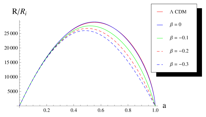
The dynamics of the collapse is shown in Fig. 7, while the linearized density contrast and the virial overdensity for various β𝛽\beta can be found in Table (2). It is important to note that the onset of the fifth term in Eq. (2) plays a crucial role in the virialisation process. In fact we can see that varying the parameter β𝛽\beta there is a substantial modification of ΔvirsubscriptΔ𝑣𝑖𝑟\Delta_{vir} with respect to the ΛCDMΛCDM\Lambda\textrm{CDM} model.

Refer to caption
Figure 7: In the figure we plot the solution of Eq. (78), in terms of the normalized radius R/Ri𝑅subscript𝑅𝑖R/R_{i} of the top-hat perturbation, when α=0𝛼0\alpha=0 and xdS=1subscript𝑥dS1x_{\rm dS}=1. The initial density for each model is shown in Tab. (2).
Model δisubscript𝛿𝑖\delta_{i} (105)superscript105(10^{-5}) δcsubscript𝛿𝑐\delta_{c} atursubscript𝑎𝑡𝑢𝑟a_{tur} Rtur/Risubscript𝑅𝑡𝑢𝑟subscript𝑅𝑖R_{tur}/R_{i} ΔtursubscriptΔ𝑡𝑢𝑟\Delta_{tur} avirsubscript𝑎𝑣𝑖𝑟a_{vir} Rvir/Risubscript𝑅𝑣𝑖𝑟subscript𝑅𝑖R_{vir}/R_{i} ΔvirsubscriptΔ𝑣𝑖𝑟\Delta_{vir}
ΛCDMΛCDM\Lambda\textrm{CDM} 2.220 1.674 0.553 28840 42 0.919 13910 371
β=0𝛽0\beta=0 2.205 1.689 0.551 28990 41 0.914 14170 351
β=0.005𝛽0.005\beta=-0.005 2.219 1.700 0.547 28800 42 0.907 14410 334
β=0.01𝛽0.01\beta=-0.01 2.227 1.707 0.544 28680 42 0.911 13810 380
β=0.02𝛽0.02\beta=-0.02 2.238 1.717 0.540 28500 43 0.910 13600 398
β=0.05𝛽0.05\beta=-0.05 2.263 1.742 0.531 28120 45 0.895 14050 361
β=0.07𝛽0.07\beta=-0.07 2.277 1.757 0.527 27910 46 0.883 14470 330
β=0.1𝛽0.1\beta=-0.1 2.296 1.780 0.520 27620 47 0.866 15060 293
β=0.2𝛽0.2\beta=-0.2 2.356 1.857 0.501 26740 52 0.813 16440 225
β=0.3𝛽0.3\beta=-0.3 2.412 1.928 0.484 25980 57 0.769 17150 198
Table 2: Here we show numerical results of physically interesting quantities, in the case α=0𝛼0\alpha=0, xdS=1subscript𝑥dS1x_{\rm dS}=1 for various β𝛽\beta

5.2.3 Case α0𝛼0\alpha\neq 0, β0𝛽0\beta\neq 0, xdS=1subscript𝑥dS1x_{\rm dS}=1.

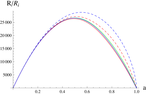
This is the most general case, despite the assumption xdS=1subscript𝑥dS1x_{\rm dS}=1. Here we can evaluate the sum of the contribution of the terms 4subscript4{\cal L}_{4} and 5subscript5{\cal L}_{5}, Eqs. (6) and (7), in the whole parameter region defined by Eq. (68). It can be noted that as α𝛼\alpha and β𝛽\beta grow we obtain a larger δcsubscript𝛿𝑐\delta_{c}, thus it should be easy to remove a large piece of parameter space from the allowed region.
Refer to caption
Figure 8: In the figure we plot the solution of Eq. (78), in terms of the normalized radius R/Ri𝑅subscript𝑅𝑖R/R_{i} of the top-hat perturbation, when α0𝛼0\alpha\neq 0, β0𝛽0\beta\neq 0 and xdS=1subscript𝑥dS1x_{\rm dS}=1. The initial density for each model is shown in Tab. (3). The values for (α,β)𝛼𝛽(\alpha,\beta) are: ΛCDMΛCDM\Lambda\textrm{CDM} blue dashed line; (0.45,0.4)0.450.4(-0.45,-0.4) red line; (0.2,0.2)0.20.2(-0.2,-0.2) green line; (0.55,0.4)0.550.4(-0.55,-0.4) blue thick line; (0.1,0.1)0.10.1(0.1,-0.1) red dashed line.
Model δisubscript𝛿𝑖\delta_{i} (105)superscript105(10^{-5}) δcsubscript𝛿𝑐\delta_{c} atursubscript𝑎𝑡𝑢𝑟a_{tur} Rtur/Risubscript𝑅𝑡𝑢𝑟subscript𝑅𝑖R_{tur}/R_{i} ΔtursubscriptΔ𝑡𝑢𝑟\Delta_{tur} avirsubscript𝑎𝑣𝑖𝑟a_{vir} Rvir/Risubscript𝑅𝑣𝑖𝑟subscript𝑅𝑖R_{vir}/R_{i} ΔvirsubscriptΔ𝑣𝑖𝑟\Delta_{vir}
ΛCDMΛCDM\Lambda\textrm{CDM} 2.220 1.674 0.553 28840 42 0.919 13910 371
α𝛼\alpha β𝛽\beta
0.10.10.1 0.10.1-0.1 2.323 1.815 0.511 27220 50 0.862 14760 311
0.20.2-0.2 0.20.2-0.2 2.356 1.831 0.499 26710 52 0.791 17230 195
0.450.45-0.45 0.40.4-0.4 2.383 1.875 0.492 26400 54 0.763 17820 177
0.550.55-0.55 0.40.4-0.4 2.362 1.851 0.496 26660 53 0.773 17710 180
Table 3: Here we show numerical results of physically interesting quantities in the case α=0𝛼0\alpha=0, xdS=1subscript𝑥dS1x_{\rm dS}=1 for various β𝛽\beta

6 Conclusions

In this paper we have first reviewed the background evolution of the Galileon model, following the tracker solution of [30]. We have found two analytic functions that describe the evolution of the components of the universe at late-times. The peculiarity of this tracker solution is that it ensures a dS stable point independent of the cisubscript𝑐𝑖c_{i} parameters of Eq. (2). This assumption simplifies our equations, but it should also be easy to generalize our work to a more general background evolution. Once c1subscript𝑐1c_{1} is set to zero, in Eq. (2) should remain only kinetic terms for the scalar field, thus the Galileon cannot be considered as a deviation from the ΛCDMΛCDM\Lambda\textrm{CDM} model. It should work as a substitute of the cosmological constant, mimicking the effects of ΛΛ\Lambda on cosmological scales.
Then we have shown that, in the linear approximation the scalr perturbations of a FRLW universe lead to a time-dependent gravitational constant Gϕ(t)subscript𝐺italic-ϕ𝑡G_{\phi}(t), that modifies the gravitational potential generated by a distant or, equivalently, small source. The results we give do not represent a realistic model, i.e. they are not required to satisfy the observational bounds, rather they are chosen on order to display what one can generally expect from this theory.
The Galileon model can be successful because it possesses a Vainshtein mechanism, by which we can consider two distinct regions; the first one at large scales, where the linear approximation applies and the Galileon drives the cosmic acceleration, the second one where non-linearities are dominant. We have also shown how to recover a Vainshtein radius in agreement with the one of DGP and other simpler models.
Even though the study of the perturbations in a highly non-linear regime can notbe completely analytic, we found some constraints, whose fulfillment allows Eq. (60) to have at least a couple of real solutions.
The last part of this paper was devoted to the study of the collapse of a spherical top-hat matter perturbation. We have shown that the new terms 4subscript4{\cal L}_{4} and 5subscript5{\cal L}_{5} affect in a non-negligible way the dynamics of the collapse and the value of δcsubscript𝛿𝑐\delta_{c} and ΔvirsubscriptΔ𝑣𝑖𝑟\Delta_{vir}. To study the virialisation process we paid attention to the energy non-conservation problem, calculating point by point the virial condition Eq. (80).

Acknowledgments

We thank Daniele Bertacca, Bin Hu, Massimo Pietroni, José M. Martín-García and the community of the Mathematica package xAct for useful discussions.

Appendix A Components of the field equations (8-10)

The terms of the stress-energy tensor of the scalar field read

Tμν(1)subscriptsuperscript𝑇1𝜇𝜈\displaystyle T^{(1)}_{\phantom{(1)}\mu\nu} =\displaystyle= 12M3gμνϕ12superscript𝑀3subscript𝑔𝜇𝜈italic-ϕ\displaystyle\frac{1}{2}M^{3}g_{\mu\nu}\,\phi (91)
Tμν(2)subscriptsuperscript𝑇2𝜇𝜈\displaystyle T^{(2)}_{\phantom{(2)}\mu\nu} =\displaystyle= ϕ;μϕ;ν+12gμν(ϕ)2\displaystyle-\phi_{;\mu}\,\phi_{;\nu}+\frac{1}{2}g_{\mu\nu}\,(\nabla\phi)^{2} (92)
Tμν(3)subscriptsuperscript𝑇3𝜇𝜈\displaystyle T^{(3)}_{\phantom{(3)}\mu\nu} =\displaystyle= 1M3[ϕ;μϕ;νϕϕ;{μϕ;ν}αϕ;α+gμνϕ;αϕ;αβϕ;β]\displaystyle-\frac{1}{M^{3}}\left[\phi_{;\mu}\,\phi_{;\nu}\,\square\phi-\phi_{;\{\mu}\,\phi_{;\nu\}\alpha}\,\phi^{;\alpha}+g_{\mu\nu}\,\phi^{;\alpha}\,\phi_{;\alpha\beta}\,\phi^{;\beta}\right] (93)
Tμν(4)subscriptsuperscript𝑇4𝜇𝜈\displaystyle T^{(4)}_{\phantom{(4)}\mu\nu} =\displaystyle= 2M6[12Rϕ;μϕ;ν(ϕ)2+2ϕ;μαϕ;αϕ;νβϕ;β+\displaystyle-\frac{2}{M^{6}}\left[-\frac{1}{2}R\,\phi_{;\mu}\,\phi_{;\nu}\,(\nabla\phi)^{2}+2\phi_{;\mu\alpha}\,\phi^{;\alpha}\,\phi_{;\nu\beta}\,\phi^{;\beta}+\right. (94)
2ϕ;μνϕ;αϕ;αβϕ;β+2ϕ;{μϕ;ν}αϕ;βϕ;βαϕ;μϕ;νϕ;αβϕ;αβ+\displaystyle\left.-2\phi_{;\mu\nu}\,\phi^{;\alpha}\,\phi_{;\alpha\beta}\,\phi^{;\beta}+2\phi_{;\{\mu}\,\phi_{;\nu\}\alpha}\,\phi_{;\beta}\,\phi^{;\beta\alpha}-\phi_{;\mu}\,\phi_{;\nu}\,\phi_{;\alpha\beta}\,\phi^{;\alpha\beta}+\right.
+Rα{μϕ;ν}ϕ;α(ϕ)214Gμν(ϕ)4+ϕ;μαϕ;να(ϕ)2+\displaystyle\left.+R_{\alpha\{\mu}\,\phi_{;\nu\}}\,\phi^{;\alpha}\,(\nabla\phi)^{2}-\frac{1}{4}G_{\mu\nu}(\nabla\phi)^{4}+\phi_{;\mu\alpha}\,\phi_{;\nu}^{\phantom{;\nu}\alpha}\,(\nabla\phi)^{2}+\right.
gμνRαβϕ;αϕ;β(ϕ)2+Rμανβϕ;αϕ;β(ϕ)2+\displaystyle\left.-g_{\mu\nu}\,R_{\alpha\beta}\,\phi^{;\alpha}\,\phi^{;\beta}\,(\nabla\phi)^{2}+R_{\mu\alpha\nu\beta}\,\phi^{;\alpha}\,\phi^{;\beta}\,(\nabla\phi)^{2}+\right.
2gμνϕ;αϕ;βϕ;βγϕ;αγϕ;μνϕ(ϕ)22ϕ;{μϕ;ν}αϕ;αϕ+\displaystyle\left.-2g_{\mu\nu}\,\phi_{;\alpha}\,\phi^{;\beta}\,\phi_{;\beta\gamma}\,\phi^{;\alpha\gamma}-\phi_{;\mu\nu}\,\square\phi\,(\nabla\phi)^{2}-2\phi_{;\{\mu}\,\phi_{;\nu\}\alpha}\,\phi^{;\alpha}\,\square\phi+\right.
+ϕ;μϕ;ν(ϕ)212gμνϕ;αβϕ;αβ(ϕ)2+2gμνϕ;αϕ;αβϕ;βϕ+\displaystyle\left.+\phi_{;\mu}\,\phi_{;\nu}\,(\square\phi)^{2}-\frac{1}{2}g_{\mu\nu}\,\phi_{;\alpha\beta}\,\phi^{;\alpha\beta}\,(\nabla\phi)^{2}+2g_{\mu\nu}\,\phi^{;\alpha}\,\phi_{;\alpha\beta}\,\phi^{;\beta}\,\square\phi+\right.
+12gμν(ϕ)2(ϕ)2]\displaystyle\left.+\frac{1}{2}g_{\mu\nu}\,(\square\phi)^{2}\,(\nabla\phi)^{2}\right]
Tμν(5)subscriptsuperscript𝑇5𝜇𝜈\displaystyle T^{(5)}_{\phantom{(5)}\mu\nu} =\displaystyle= 2M9[3ϕ;μγϕ;νγϕ;αϕ;αβϕ;β3ϕ;μαϕ;νγϕ;γϕ;βϕ;βα+\displaystyle-\frac{2}{M^{9}}\left[3\phi_{;\mu\gamma}\,\phi_{;\nu}^{\phantom{;\nu}\gamma}\,\phi^{;\alpha}\,\phi_{;\alpha\beta}\,\phi^{;\beta}-3\phi_{;\mu\alpha}\,\phi_{;\nu\gamma}\,\phi^{;\gamma}\,\phi_{;\beta}\,\phi^{;\beta\alpha}+\right. (95)
+32ϕ;μνRαβϕ;αϕ;β(ϕ)232Rα{μϕ;ν}βϕ;αϕ;β(ϕ)2+\displaystyle\left.+\frac{3}{2}\phi_{;\mu\nu}\,R_{\alpha\beta}\,\phi^{;\alpha}\,\phi^{;\beta}\,(\nabla\phi)^{2}-\frac{3}{2}R_{\alpha\{\mu}\,\phi_{;\nu\}\beta}\,\phi^{;\alpha}\,\phi^{;\beta}\,(\nabla\phi)^{2}+\right.
+34Rϕ;{μϕ;ν}αϕ;α(ϕ)2+32Gμνϕ;αϕ;αβϕ;β(ϕ)2+\displaystyle\left.+\frac{3}{4}R\,\phi_{;\{\mu}\,\phi_{;\nu\}\alpha}\,\phi^{;\alpha}\,(\nabla\phi)^{2}+\frac{3}{2}G_{\mu\nu}\,\phi^{;\alpha}\,\phi_{;\alpha\beta}\,\phi^{;\beta}\,(\nabla\phi)^{2}+\right.
32Rβαϕ;{μϕ;ν}αϕ;β(ϕ)23ϕ;μαϕ;νβϕ;αϕ;γϕ;βγ+\displaystyle\left.-\frac{3}{2}R_{\beta}^{\phantom{\beta}\alpha}\,\phi_{;\{\mu}\,\phi_{;\nu\}\alpha}\,\phi^{;\beta}\,(\nabla\phi)^{2}-3\phi_{;\mu\alpha}\,\phi_{;\nu\beta}\,\phi^{;\alpha}\,\phi_{;\gamma}\,\phi^{;\beta\gamma}+\right.
3ϕ;μαϕ;αβϕ;νβ(ϕ)2+3ϕ;μνϕ;αϕ;αβϕ;γβϕ;γ+\displaystyle\left.-3\phi_{;\mu\alpha}\,\phi^{;\alpha\beta}\,\phi_{;\nu\beta}\,(\nabla\phi)^{2}+3\phi_{;\mu\nu}\,\phi_{;\alpha}\,\phi^{;\alpha\beta}\,\phi_{;\gamma\beta}\,\phi^{;\gamma}+\right.
3ϕ;{μϕ;ν}αϕ;αβϕ;γβϕ;γ+32Rαβϕ;μϕ;νϕ;αβ(ϕ)2+\displaystyle\left.-3\phi_{;\{\mu}\,\phi_{;\nu\}\alpha}\,\phi^{;\alpha\beta}\,\phi_{;\gamma\beta}\,\phi^{;\gamma}+\frac{3}{2}R_{\alpha\beta}\,\phi_{;\mu}\,\phi_{;\nu}\,\phi^{;\alpha\beta}\,(\nabla\phi)^{2}+\right.
+ϕ;μϕ;νϕ;αβϕ;βγϕ;αγ+34Rϕ;μϕ;νϕ(ϕ)2+\displaystyle\left.+\phi_{;\mu}\,\phi_{;\nu}\,\phi_{;\alpha}^{\phantom{;\alpha}\beta}\,\phi_{;\beta\gamma}\,\phi^{;\alpha\gamma}+\frac{3}{4}R\,\phi_{;\mu}\,\phi_{;\nu}\,\square\phi\,(\nabla\phi)^{2}+\right.
+32ϕ;μνϕ;αβϕ;αβ(ϕ)2+32ϕ;{μϕ;ν}αϕ;αϕ;βγϕ;βγ+\displaystyle\left.+\frac{3}{2}\phi_{;\mu\nu}\,\phi_{;\alpha\beta}\,\phi^{;\alpha\beta}\,(\nabla\phi)^{2}+\frac{3}{2}\phi_{;\{\mu}\,\phi_{;\nu\}\alpha}\,\phi^{;\alpha}\,\phi_{;\beta\gamma}\,\phi^{;\beta\gamma}+\right.
32ϕ;μϕ;νϕ;αβϕ;αβϕ+32Rαγβ{μϕ;ν}αϕ;βϕ;γ(ϕ)2+\displaystyle\left.-\frac{3}{2}\phi_{;\mu}\,\phi_{;\nu}\,\phi_{;\alpha\beta}\,\phi^{;\alpha\beta}\,\square\phi+\frac{3}{2}R_{\alpha\gamma\beta\{\mu}\,\phi_{;\nu\}}^{\phantom{;\nu\}}\alpha}\,\phi^{;\beta}\,\phi^{;\gamma}\,(\nabla\phi)^{2}+\right.
32Rα{μϕ;ν}ϕ;βϕ;βα(ϕ)232Rαγβ{μϕ;ν}ϕ;γϕ;αβ(ϕ)2+\displaystyle\left.-\frac{3}{2}R_{\alpha\{\mu}\,\phi_{;\nu\}}\,\phi_{;\beta}\,\phi^{;\beta\alpha}\,(\nabla\phi)^{2}-\frac{3}{2}R_{\alpha\gamma\beta\{\mu}\,\phi_{;\nu\}}\,\phi^{;\gamma}\,\phi^{;\alpha\beta}\,(\nabla\phi)^{2}+\right.
32Rϕ;μϕ;νϕ(ϕ)2+32Rα{μϕ;ν}ϕ;αϕ(ϕ)2+\displaystyle\left.-\frac{3}{2}R\,\phi_{;\mu}\,\phi_{;\nu}\,\square\phi\,(\nabla\phi)^{2}+\frac{3}{2}R_{\alpha\{\mu}\,\phi_{;\nu\}}\,\phi^{;\alpha}\,\square\phi\,(\nabla\phi)^{2}+\right.
+3gμνϕ;αϕ;βϕ;αγϕ;γτϕ;βτ+3gμνRγβϕ;αϕ;γϕ;αβ(ϕ)2+\displaystyle\left.+3g_{\mu\nu}\,\phi_{;\alpha}\,\phi_{;\beta}\,\phi^{;\alpha\gamma}\,\phi_{;\gamma\tau}\,\phi^{;\beta\tau}+3g_{\mu\nu}\,R_{\gamma\beta}\,\phi_{;\alpha}\,\phi^{;\gamma}\,\phi^{;\alpha\beta}\,(\nabla\phi)^{2}+\right.
32Rμναβϕ;γϕ;αϕ;βγ(ϕ)23Rμβνγϕ;αϕ;γϕ;αβ(ϕ)2+\displaystyle\left.-\frac{3}{2}R_{\mu\nu\alpha\beta}\,\phi_{;\gamma}\,\phi^{;\alpha}\,\phi^{;\beta\gamma}\,(\nabla\phi)^{2}-3R_{\mu\beta\nu\gamma}\,\phi_{;\alpha}\,\phi^{;\gamma}\,\phi^{;\alpha\beta}\,(\nabla\phi)^{2}+\right.
+32gμνRαγβτϕ;αϕ;βϕ;γτ(ϕ)2+gμνϕβ;αϕ;αγϕ;βγ(ϕ)2+\displaystyle\left.+\frac{3}{2}g_{\mu\nu}\,R_{\alpha\gamma\beta\tau}\,\phi^{;\alpha}\,\phi^{;\beta}\,\phi^{;\gamma\tau}\,(\nabla\phi)^{2}+g_{\mu\nu}\,\phi^{;\alpha}_{\phantom{;\alpha}\beta}\,\phi_{;\alpha\gamma}\,\phi^{;\beta\gamma}\,(\nabla\phi)^{2}+\right.
+3ϕ;μαϕ;αϕ;νβϕ;βϕ3ϕ;μνϕ;αϕ;αβϕ;βϕ+\displaystyle\left.+3\phi_{;\mu\alpha}\,\phi^{;\alpha}\,\phi_{;\nu\beta}\,\phi^{;\beta}\,\square\phi-3\phi_{;\mu\nu}\,\phi^{;\alpha}\,\phi_{;\alpha\beta}\,\phi^{;\beta}\,\square\phi+\right.
+3ϕ;{μϕ;ν}αϕ;βαϕ;βϕ+3ϕ;μαϕ;ναϕ(ϕ)2+\displaystyle\left.+3\phi_{;\{\mu}\,\phi_{;\nu\}\alpha}\,\phi^{;\beta\alpha}\,\phi_{;\beta}\,\square\phi+3\phi_{;\mu\alpha}\,\phi_{;\nu}^{\phantom{;\nu}\alpha}\,\square\phi\,(\nabla\phi)^{2}+\right.
32gμνRαβϕ;αϕ;βϕ(ϕ)2+32Rμανβϕ;αϕ;βϕ(ϕ)2+\displaystyle\left.-\frac{3}{2}g_{\mu\nu}\,R_{\alpha\beta}\,\phi^{;\alpha}\,\phi^{;\beta}\,\square\phi\,(\nabla\phi)^{2}+\frac{3}{2}R_{\mu\alpha\nu\beta}\,\phi^{;\alpha}\,\phi^{;\beta}\,\square\phi\,(\nabla\phi)^{2}+\right.
32ϕ;μν(ϕ)2(ϕ)232ϕ;{μϕ;ν}αϕ;α(ϕ)2+12ϕ;μϕ;ν(ϕ)3+\displaystyle\left.-\frac{3}{2}\phi_{;\mu\nu}\,(\square\phi)^{2}\,(\nabla\phi)^{2}-\frac{3}{2}\phi_{;\{\mu}\,\phi_{;\nu\}\alpha}\,\phi^{;\alpha}\,(\square\phi)^{2}+\frac{1}{2}\phi_{;\mu}\,\phi_{;\nu}\,(\square\phi)^{3}+\right.
32gμνϕ;αϕ;αβϕ;βϕ;γτϕ;γτ32gμνϕ;αβϕ;αβϕ(ϕ)2+\displaystyle\left.-\frac{3}{2}g_{\mu\nu}\,\phi^{;\alpha}\,\phi_{;\alpha\beta}\,\phi^{;\beta}\,\phi_{;\gamma\tau}\,\phi^{;\gamma\tau}-\frac{3}{2}g_{\mu\nu}\,\phi_{;\alpha\beta}\,\phi^{;\alpha\beta}\,\square\phi\,(\nabla\phi)^{2}+\right.
3gμνϕ;αϕ;γϕ;γβϕ;αβϕ+32gμνϕ;αϕ;αβϕ;β(ϕ)2+\displaystyle\left.-3g_{\mu\nu}\,\phi_{;\alpha}\,\phi^{;\gamma}\,\phi_{;\gamma\beta}\,\phi^{;\alpha\beta}\,\square\phi+\frac{3}{2}g_{\mu\nu}\,\phi^{;\alpha}\,\phi_{;\alpha\beta}\,\phi^{;\beta}\,(\square\phi)^{2}+\right.
+12gμν(ϕ)3(ϕ)2].\displaystyle\left.+\frac{1}{2}g_{\mu\nu}(\square\phi)^{3}(\nabla\phi)^{2}\right].

The terms appearing in the equation of motion for the scalar field read

ξ(1)superscript𝜉1\displaystyle\xi^{(1)} =\displaystyle= M32superscript𝑀32\displaystyle\frac{M^{3}}{2} (96)
ξ(2)superscript𝜉2\displaystyle\xi^{(2)} =\displaystyle= ϕitalic-ϕ\displaystyle-\square\phi (97)
ξ(3)superscript𝜉3\displaystyle\xi^{(3)} =\displaystyle= 1M3[(ϕ)2+Rμνϕ;μϕ;ν+ϕ;μνϕ;μν]\displaystyle\frac{1}{M^{3}}\left[-(\square\phi)^{2}+R_{\mu\nu}\,\phi^{;\mu}\,\phi^{;\nu}+\phi_{;\mu\nu}\,\phi^{;\mu\nu}\right] (98)
ξ(4)superscript𝜉4\displaystyle\xi^{(4)} =\displaystyle= 1M6[2Rϕ;μϕ;μνϕ;ν8Rναϕ;μϕ;νϕ;μα2Rμνϕ;μν(ϕ)2+\displaystyle\frac{1}{M^{6}}\left[2R\,\phi^{;\mu}\,\phi_{;\mu\nu}\,\phi^{;\nu}-8R_{\nu\alpha}\,\phi^{;\mu}\,\phi^{;\nu}\,\phi_{;\mu}^{\phantom{;\mu}\alpha}-2R_{\mu\nu}\,\phi^{;\mu\nu}\,(\nabla\phi)^{2}+\right. (99)
4Rμανβϕ;μϕ;νϕ;αβ4ϕ;μνϕ;ναϕα;μ+R(ϕ)2ϕ+\displaystyle\left.-4R_{\mu\alpha\nu\beta}\,\phi^{;\mu}\,\phi^{;\nu}\,\phi^{;\alpha\beta}-4\phi_{;\mu}^{\phantom{;\mu}\nu}\,\phi_{;\nu}^{\phantom{;\nu}\alpha}\,\phi^{;\mu}_{\phantom{;\mu}\alpha}+R\,(\nabla\phi)^{2}\,\square\phi+\right.
+4Rμνϕ;μϕ;νϕ+6ϕ;μνϕ;μνϕ2(ϕ)3]\displaystyle\left.+4R_{\mu\nu}\,\phi^{;\mu}\,\phi^{;\nu}\,\square\phi+6\phi_{;\mu\nu}\,\phi^{;\mu\nu}\,\square\phi-2(\square\phi)^{3}\right]
ξ(5)superscript𝜉5\displaystyle\xi^{(5)} =\displaystyle= 1M9[32R(ϕ)2(ϕ)2+3Rϕ;μϕ;μνϕ;νϕ+\displaystyle\frac{1}{M^{9}}\left[\frac{3}{2}R\,(\nabla\phi)^{2}\,(\square\phi)^{2}+3R\,\phi^{;\mu}\,\phi_{;\mu\nu}\,\phi^{;\nu}\,\square\phi+\right. (100)
+3RμαRναϕ;μϕ;ν(ϕ)232RRμνϕ;μϕ;ν(ϕ)2+\displaystyle\left.+3R_{\mu}^{\phantom{\mu}\alpha}\,R_{\nu\alpha}\,\phi^{;\mu}\,\phi^{;\nu}\,(\nabla\phi)^{2}-\frac{3}{2}R\,R_{\mu\nu}\,\phi^{;\mu}\,\phi^{;\nu}\,(\nabla\phi)^{2}+\right.
+3RμνRαμβνϕ;αϕ;β(ϕ)232RμαβγRναβγϕ;μϕ;ν(ϕ)2+\displaystyle\left.+3R^{\mu\nu}\,R_{\alpha\mu\beta\nu}\,\phi^{;\alpha}\,\phi^{;\beta}\,(\nabla\phi)^{2}-\frac{3}{2}R_{\mu}^{\phantom{\mu}\alpha\beta\gamma}\,R_{\nu\alpha\beta\gamma}\,\phi^{;\mu}\,\phi^{;\nu}\,(\nabla\phi)^{2}+\right.
3Rϕ;μϕ;νϕ;μαϕ;μα32Rϕ;μνϕ;μν(ϕ)2(ϕ)4+\displaystyle\left.-3R\,\phi^{;\mu}\,\phi^{;\nu}\,\phi_{;\mu\alpha}\,\phi_{;\mu}^{\phantom{;\mu}\alpha}-\frac{3}{2}R\,\phi_{;\mu\nu}\,\phi^{;\mu\nu}\,(\nabla\phi)^{2}-(\square\phi)^{4}+\right.
+3Rμνϕ;μϕ;ν(ϕ)212Rμαϕ;μϕ;νϕ;ναϕ+\displaystyle\left.+3R_{\mu\nu}\,\phi^{;\mu}\,\phi^{;\nu}\,(\square\phi)^{2}-12R_{\mu\alpha}\,\phi^{;\mu}\,\phi^{;\nu}\,\phi_{;\nu}^{\phantom{;\nu}\alpha}\,\square\phi+\right.
+6Rαβϕ;μϕ;νϕ;μαϕ;νβ+6Rμνϕ;μαϕ;αν(ϕ)2+\displaystyle\left.+6R_{\alpha\beta}\,\phi^{;\mu}\,\phi^{;\nu}\,\phi_{;\mu}^{\phantom{;\mu}\alpha}\,\phi_{;\nu}^{\phantom{;\nu}\beta}+6R_{\mu\nu}\,\phi^{;\mu\alpha}\,\phi_{;\alpha}^{\phantom{;\alpha}\nu}\,(\nabla\phi)^{2}+\right.
+6ϕ;μνϕ;μαϕ;αβϕ;νβ8ϕ;μνϕ;ναϕ;μαϕ+\displaystyle\left.+6\phi^{;\mu\nu}\,\phi_{;\mu\alpha}\,\phi^{;\alpha\beta}\,\phi_{;\nu\beta}-8\phi^{;\mu\nu}\,\phi_{;\nu\alpha}\,\phi_{;\mu}^{\phantom{;\mu}\alpha}\,\square\phi+\right.
+12Rνβϕ;μϕ;νϕ;μαϕ;αβ6Rμνϕ;μν(ϕ)2ϕ+\displaystyle\left.+12R_{\nu\beta}\,\phi^{;\mu}\phi^{;\nu}\,\phi_{;\mu\alpha}\,\phi^{;\alpha\beta}-6R_{\mu\nu}\,\phi^{;\mu\nu}\,(\nabla\phi)^{2}\,\square\phi+\right.
6Rμνϕ;μνϕ;αϕ;αβϕ;β+6ϕ;μνϕ;μν(ϕ)23Rαβϕ;αϕ;βϕ;μνϕ;μν+\displaystyle\left.-6R_{\mu\nu}\,\phi^{;\mu\nu}\,\phi^{;\alpha}\,\phi_{;\alpha\beta}\,\phi^{;\beta}+6\phi_{;\mu\nu}\,\phi^{;\mu\nu}\,(\square\phi)^{2}-3R_{\alpha\beta}\,\phi^{;\alpha}\,\phi^{;\beta}\,\phi_{;\mu\nu}\,\phi^{;\mu\nu}+\right.
3(ϕ;μνϕ;μν)2+6Rμανβϕ;μϕ;νϕ;γαϕ;γβ6Rμανβϕ;μϕ;νϕ;αβϕ+\displaystyle\left.-3(\phi_{;\mu\nu}\,\phi^{;\mu\nu})^{2}+6R_{\mu\alpha\nu\beta}\,\phi^{;\mu}\,\phi^{;\nu}\,\phi^{;\gamma\alpha}\,\phi_{;\gamma}^{\phantom{;\gamma}\beta}-6R_{\mu\alpha\nu\beta}\,\phi^{;\mu}\,\phi^{;\nu}\,\phi^{;\alpha\beta}\,\square\phi+\right.
+12Rμανβϕ;γϕ;μϕ;γνϕ;αβ+3Rμανβϕ;μνϕ;αβ(ϕ)2]\displaystyle\left.+12R_{\mu\alpha\nu\beta}\,\phi^{;\gamma}\,\phi^{;\mu}\,\phi_{;\gamma}^{\phantom{;\gamma}\nu}\,\phi^{;\alpha\beta}+3R_{\mu\alpha\nu\beta}\,\phi^{;\mu\nu}\,\phi^{;\alpha\beta}\,(\nabla\phi)^{2}\right]

Appendix B Background functions

Background functions involved in the linear perturbation theory:

γ1(t)subscript𝛾1𝑡\displaystyle\gamma_{1}(t) \displaystyle\equiv 3(α2xdSβ)ϕ˙2HdS4Mpl23𝛼2subscript𝑥dS𝛽superscript˙italic-ϕ2superscriptsubscript𝐻dS4superscriptsubscript𝑀pl2\displaystyle 3\left(\alpha-2x_{\rm dS}\beta\right)\frac{\dot{\phi}^{2}}{H_{\rm dS}^{4}M_{\rm pl}^{2}} (101)
γ2(t)subscript𝛾2𝑡\displaystyle\gamma_{2}(t) \displaystyle\equiv (2+9α9β12xdSα+15xdS2β)ϕ˙2HdS2Mpl29𝛼9𝛽12subscript𝑥dS𝛼15superscriptsubscript𝑥dS2𝛽superscript˙italic-ϕ2superscriptsubscript𝐻dS2subscript𝑀pl\displaystyle\left(2+9\alpha-9\beta-12x_{\rm dS}\alpha+15x_{\rm dS}^{2}\beta\right)\frac{\dot{\phi}^{2}}{H_{\rm dS}^{2}M_{\rm pl}} (102)
γ3(t)subscript𝛾3𝑡\displaystyle\gamma_{3}(t) \displaystyle\equiv ϕ˙43HdS4Mpl2(α+6βϕ¨HdS2Mpl)superscript˙italic-ϕ43superscriptsubscript𝐻dS4superscriptsubscript𝑀pl2𝛼6𝛽¨italic-ϕsuperscriptsubscript𝐻dS2subscript𝑀pl\displaystyle-\frac{\dot{\phi}^{4}}{3H_{\rm dS}^{4}M_{\rm pl}^{2}}\left(\alpha+6\beta\frac{\ddot{\phi}}{H_{\rm dS}^{2}M_{\rm pl}}\right) (103)
γ4(t)subscript𝛾4𝑡\displaystyle\gamma_{4}(t) \displaystyle\equiv 2ϕ˙23HdS2Mpl(2α3xdSβ)(xdS+3ϕ¨HdS2Mpl)2superscript˙italic-ϕ23superscriptsubscript𝐻dS2subscript𝑀pl2𝛼3subscript𝑥dS𝛽subscript𝑥dS3¨italic-ϕsuperscriptsubscript𝐻dS2subscript𝑀pl\displaystyle-\frac{2\dot{\phi}^{2}}{3H_{\rm dS}^{2}M_{\rm pl}}\left(2\alpha-3x_{\rm dS}\beta\right)\left(x_{\rm dS}+\frac{3\ddot{\phi}}{H_{\rm dS}^{2}M_{\rm pl}}\right) (104)
γ5(t)subscript𝛾5𝑡\displaystyle\gamma_{5}(t) \displaystyle\equiv 69α+12β26xdS2α+4xdS(2+9α9β)+24xdS3β+69𝛼12𝛽26superscriptsubscript𝑥dS2𝛼4subscript𝑥dS29𝛼9𝛽limit-from24superscriptsubscript𝑥dS3𝛽\displaystyle-6-9\alpha+12\beta-26x_{\rm dS}^{2}\alpha+4x_{\rm dS}\left(2+9\alpha-9\beta\right)+24x_{\rm dS}^{3}\beta+ (105)
+2[2+9α9β6xdS(αxdSβ)]ϕ¨HdS2Mpl2delimited-[]29𝛼9𝛽6subscript𝑥dS𝛼subscript𝑥dS𝛽¨italic-ϕsuperscriptsubscript𝐻dS2subscript𝑀pl\displaystyle+2\left[2+9\alpha-9\beta-6x_{\rm dS}\left(\alpha-x_{\rm dS}\beta\right)\right]\frac{\ddot{\phi}}{H_{\rm dS}^{2}M_{\rm pl}}

Background functions involved in the non-linear dynamics:

η1(t)subscript𝜂1𝑡\displaystyle\eta_{1}(t) \displaystyle\equiv 2βHdS6Mpl3ϕ˙22𝛽superscriptsubscript𝐻dS6superscriptsubscript𝑀pl3superscript˙italic-ϕ2\displaystyle\frac{2\beta}{H_{\rm dS}^{6}M_{\rm pl}^{3}}\dot{\phi}^{2} (106)
η2(t)subscript𝜂2𝑡\displaystyle\eta_{2}(t) \displaystyle\equiv ϕ˙23HdS4Mpl2(α6βϕ¨HdS2Mpl)superscript˙italic-ϕ23superscriptsubscript𝐻dS4superscriptsubscript𝑀pl2𝛼6𝛽¨italic-ϕsuperscriptsubscript𝐻dS2subscript𝑀pl\displaystyle\frac{\dot{\phi}^{2}}{3H_{\rm dS}^{4}M_{\rm pl}^{2}}\left(\alpha-6\beta\frac{\ddot{\phi}}{H_{\rm dS}^{2}M_{\rm pl}}\right) (107)
η3(t)subscript𝜂3𝑡\displaystyle\eta_{3}(t) \displaystyle\equiv 1HdS2Mpl[2+9α9β6(αxdSβ)(xdS+ϕ¨HdS2Mpl)]1superscriptsubscript𝐻dS2subscript𝑀pldelimited-[]29𝛼9𝛽6𝛼subscript𝑥dS𝛽subscript𝑥dS¨italic-ϕsuperscriptsubscript𝐻dS2subscript𝑀pl\displaystyle\frac{1}{H_{\rm dS}^{2}M_{\rm pl}}\left[2+9\alpha-9\beta-6\left(\alpha-x_{\rm dS}\beta\right)\left(x_{\rm dS}+\frac{\ddot{\phi}}{H_{\rm dS}^{2}M_{\rm pl}}\right)\right] (108)
η4(t)subscript𝜂4𝑡\displaystyle\eta_{4}(t) \displaystyle\equiv 2HdS4Mpl2(α2βϕ¨HdS2Mpl)2superscriptsubscript𝐻dS4superscriptsubscript𝑀pl2𝛼2𝛽¨italic-ϕsuperscriptsubscript𝐻dS2subscript𝑀pl\displaystyle\frac{2}{H_{\rm dS}^{4}M_{\rm pl}^{2}}\left(\alpha-2\beta\frac{\ddot{\phi}}{H_{\rm dS}^{2}M_{\rm pl}}\right) (109)

References

References

  • [1] Supernova Cosmology Project Collaboration, S. Perlmutter et. al., Measurements of Omega and Lambda from 42 High-Redshift Supernovae, Astrophys. J. 517 (1999) 565–586, [astro-ph/9812133].
  • [2] Supernova Search Team Collaboration, A. G. Riess et. al., Observational Evidence from Supernovae for an Accelerating Universe and a Cosmological Constant, Astron. J. 116 (1998) 1009–1038, [astro-ph/9805201].
  • [3] A. G. Riess et. al., BVRI Light Curves for 22 Type Ia Supernovae, Astron. J. 117 (1999) 707–724, [astro-ph/9810291].
  • [4] C. Brans and R. H. Dicke, Mach’s principle and a relativistic theory of gravitation, Phys. Rev. 124 (1961) 925–935.
  • [5] A. De Felice and S. Tsujikawa, f(R) theories, Living Rev. Rel. 13 (2010) 3, [arXiv:1002.4928].
  • [6] K. Hinterbichler, Theoretical Aspects of Massive Gravity, arXiv:1105.3735.
  • [7] R. Maartens, Brane world cosmology, AIP Conf. Proc. 736 (2005) 21–34.
  • [8] A. Nicolis, R. Rattazzi, and E. Trincherini, The galileon as a local modification of gravity, Phys. Rev. D79 (2009) 064036, [arXiv:0811.2197].
  • [9] J. Khoury and A. Weltman, Chameleon Cosmology, Phys. Rev. D69 (2004) 044026, [astro-ph/0309411].
  • [10] T. Kobayashi, Cosmic expansion and growth histories in galileon scalar-tensor models of dark energy, Physical Review D 81 (2010), no. 10 103533.
  • [11] K. Van Acoleyen and J. Van Doorsselaere, Galileons from Lovelock actions, Phys.Rev. D83 (2011) 084025, [arXiv:1102.0487].
  • [12] G. Goon, K. Hinterbichler, and M. Trodden, Galileons on Cosmological Backgrounds, JCAP 1112 (2011) 004, [arXiv:1109.3450].
  • [13] T. Qiu, J. Evslin, Y.-F. Cai, M. Li, and X. Zhang, Bouncing Galileon Cosmologies, JCAP 1110 (2011) 036, [arXiv:1108.0593].
  • [14] X. Gao, Conserved cosmological perturbation in Galileon models, JCAP 1110 (2011) 021, [arXiv:1106.0292].
  • [15] C. Burrage, C. de Rham, and L. Heisenberg, de Sitter Galileon, JCAP 1105 (2011) 025, [arXiv:1104.0155].
  • [16] J. Khoury, J.-L. Lehners, and B. A. Ovrut, Supersymmetric Galileons, Phys.Rev. D84 (2011) 043521, [arXiv:1103.0003].
  • [17] M. Trodden and K. Hinterbichler, Generalizing Galileons, Class.Quant.Grav. 28 (2011) 204003, [arXiv:1104.2088].
  • [18] A. De Felice, R. Kase, and S. Tsujikawa, Matter perturbations in Galileon cosmology, Phys.Rev. D83 (2011) 043515, [arXiv:1011.6132].
  • [19] E. Babichev, Galileon accretion, Phys.Rev. D83 (2011) 024008, [arXiv:1009.2921].
  • [20] A. Padilla, P. M. Saffin, and S.-Y. Zhou, Bi-galileon theory I: Motivation and formulation, JHEP 1012 (2010) 031, [arXiv:1007.5424].
  • [21] T. Kobayashi, H. Tashiro, and D. Suzuki, Evolution of linear cosmological perturbations and its observational implications in Galileon-type modified gravity, Phys.Rev. D81 (2010) 063513, [arXiv:0912.4641].
  • [22] F. P. Silva and K. Koyama, Self-Accelerating Universe in Galileon Cosmology, Phys.Rev. D80 (2009) 121301, [arXiv:0909.4538].
  • [23] C. de Rham and A. J. Tolley, DBI and the Galileon reunited, JCAP 1005 (2010) 015, [arXiv:1003.5917].
  • [24] C. Deffayet, S. Deser, and G. Esposito-Farese, Arbitrary p𝑝p-form Galileons, Phys.Rev. D82 (2010) 061501, [arXiv:1007.5278].
  • [25] D. A. Easson, I. Sawicki, and A. Vikman, G-Bounce, JCAP 1111 (2011) 021, [arXiv:1109.1047]. 28 pages. v2 reflects version accepted for publication in JCAP. References and minor comments added.
  • [26] G. R. Dvali, G. Gabadadze, and M. Porrati, 4D gravity on a brane in 5D Minkowski space, Phys. Lett. B485 (2000) 208–214, [hep-th/0005016].
  • [27] C. Deffayet, G. Esposito-Farese, and A. Vikman, Covariant Galileon, Phys. Rev. D79 (2009) 084003, [arXiv:0901.1314].
  • [28] C. Deffayet, S. Deser, and G. Esposito-Farese, Generalized Galileons: All scalar models whose curved background extensions maintain second-order field equations and stress-tensors, Phys. Rev. D80 (2009) 064015, [arXiv:0906.1967].
  • [29] P. Creminelli, A. Nicolis, and E. Trincherini, Galilean Genesis: an alternative to inflation, JCAP 1011 (2010) 021, [arXiv:1007.0027].
  • [30] A. De Felice and S. Tsujikawa, Cosmology of a covariant Galileon field, Phys. Rev. Lett. 105 (2010) 111301, [arXiv:1007.2700].
  • [31] A. I. Vainshtein, To the problem of nonvanishing gravitation mass, Phys. Lett. B39 (1972) 393–394.
  • [32] N. Kaloper, A. Padilla, and N. Tanahashi, Galileon Hairs of Dyson Spheres, Vainshtein’s Coiffure and Hirsute Bubbles, arXiv:1106.4827.
  • [33] R. Kimura, T. Kobayashi, and K. Yamamoto, Vainshtein screening in a cosmological background in the most general second-order scalar-tensor theory, Phys.Rev. D85 (2012) 024023, [arXiv:1111.6749]. 12 pages, 5 figures, v2: published in PRD.
  • [34] F. Schmidt, M. V. Lima, H. Oyaizu, and W. Hu, Non-linear Evolution of f(R) Cosmologies III: Halo Statistics, Phys. Rev. D79 (2009) 083518, [arXiv:0812.0545].
  • [35] F. Schmidt, W. Hu, and M. Lima, Spherical Collapse and the Halo Model in Braneworld Gravity, Phys. Rev. D81 (2010) 063005, [arXiv:0911.5178].
  • [36] R. Kimura and K. Yamamoto, Large Scale Structures in Kinetic Gravity Braiding Model That Can Be Unbraided, JCAP 1104 (2011) 025, [arXiv:1011.2006].
  • [37] P. Creminelli, G. D’Amico, J. Norena, L. Senatore, and F. Vernizzi, Spherical collapse in quintessence models with zero speed of sound, JCAP 1003 (2010) 027, [arXiv:0911.2701].
  • [38] A. De Felice and T. Suyama, Vacuum structure for scalar cosmological perturbations in Modified Gravity Models, JCAP 0906 (2009) 034, [arXiv:0904.2092].
  • [39] A. De Felice, S. Mukohyama, and S. Tsujikawa, Density perturbations in general modified gravitational theories, Phys. Rev. D82 (2010) 023524, [arXiv:1006.0281].
  • [40] C. Burrage and D. Seery, Revisiting fifth forces in the Galileon model, JCAP 1008 (2010) 011, [arXiv:1005.1927].
  • [41] P. Brax, C. Burrage, and A.-C. Davis, Laboratory Tests of the Galileon, JCAP 1109 (2011) 020, [arXiv:1106.1573].
  • [42] A. De Felice and S. Tsujikawa, Cosmological constraints on extended Galileon models, arXiv:1112.1774.
  • [43] K. Hirano and Z. Komiya, Observational tests of Galileon gravity with growth rate, arXiv:1012.5451.
  • [44] K. Hirano, Z. Komiya, and H. Shirai, Constraining Galileon gravity from observational data, arXiv:1103.6133.