Correlations from generalized thermodynamic uncertainty relations

Abstract:

In order to account for possible nonstatistical fluctuations in a hadronizing system while using a statistical approach, one has to resort to its nonextensive version. The new parameter $q$ is introduced to be directly connected to the variance of an observable (with $q=1$ one returns to usual statistics). We demonstrate how this approach allows composing fluctuations of different observables and show that it leads to a specific sum rules proposing this to be verified experimentally. We discuss the ensembles in which all relevant quantities are allowed to fluctuate. By introducing correlations between the observables, the relations connecting these variables are shown to generalize the so-called Lindhard thermodynamic uncertainty relations. This is illustrated using multihadron production data. We show that fluctuations from different components of collision phase space are correlated and that the strength of these correlations depend on the relevant $q$-parameter.

1 Introduction

Nowadays it is a standard procedure to use a statistical approach to model high energy multiparticle production processes [1]. However, it has also been realized that data on many single particle distributions demonstrate a power-like behavior, rather than the expected simple exponential one. In addition, multiparticle distributions are broader than naively expected. The proposition put forward some time ago is that, rather than invalidating a simple statistical approach, these observations call for its modification towards inclusion of a possible intrinsic, nonstatistical fluctuations, usually identified with fluctuations of the parameter $T$ identified with the ”temperature” of the hadronizing fireball (cf. reviews [2]). The introduced parameter $q$, known as the nonextensivity parameter, is shown to be directly connected to the variance of $T$,

$$q=1+\omega_{T}^{2}\quad{\rm with}\quad\omega^{2}_{T}=\frac{Var(T)}{<T>^{2}},$$ (1)

and one obtains the so called Tsallis distribution

$$h_{q}(E)=\frac{2-q}{T}\exp_{q}\left(-\frac{E}{T}\right)=\frac{2-q}{T}\left[1-(1-q)\frac{E}{T}\right]^{\frac{1}{1-q}}\,\stackrel{{\scriptstyle q\rightarrow 1}}{{\Longrightarrow}}\,\frac{1}{T}\exp\left(-\frac{E}{T}\right).$$ (2)

It reduces to the usual Boltzmann-Gibbs form for $q=1$ (in which case one recovers the usual statistical model). Such an approach is also known as Tsallis statistics [9].

2 Results

In this presentation we shall not go into the details of Tsallis statistics and its applications in the field of multiparticle production observed in high energy experiments (see [2, 9]). Here we concentrate on the problem of the coexistence and interconnection between fluctuations observed in different observables and, in particular, on the possible correlation between them which can, presumably, be measured experimentally. In any collision one observes a number $N$ of secondaries distributed in phase space $\{y,p_{T}\}$ (with rapidity $y$ and transverse momentum $p_{T}$). The multiplicity distributions, $P(N)$, rapidity distributions, $dN/dy$ and distributions of transverse momenta, $dN/dp_{T}$ (or, transverse masses $\mu_{T}=\sqrt{m^{2}+p^{2}_{T}}$) are usually measured. Among them, only $P(N)$ refers to the entire phase space, the other are limited either to its longitudinal ($y$) or transverse ($p_{T}$) parts. Therefore it is natural that nonextensivity parameters describing fluctuations present in these observables (visible either as a broadening of $P(N)$ or power-like tails in other distributions) are different. This is clear from Fig. 1 where we show that, whereas fluctuations in full phase space depends strongly on energy, those confined to its transverse part depend on energy weakly. Fluctuations in the longitudinal part of phase space represent a special case as they strongly depend on data from which they are deduced and also on whether they are corrected for simultaneous fluctuations in $p_{T}$ or not [10]. This is shown in Fig. 1 by the star symbols. As shown in [11], all these fluctuations can be connected when one considers an ensemble in which all variables characterizing an event, namely, the energy $U$, temperature $T$ and multiplicity $N$, can fluctuate with relative variance $\omega^{2}_{X}=Var(X)/<X>^{2}$, $X=U,~{}T,~{}N$. In this case, it occurs in a natural way that a correlation coefficient $\rho=Cov(U,T)/\sqrt{Var(U)Var(T)}$ between the two of them (here $U$ and $T$ chosen) is necessary to fully describe the event. Generalizing the Lindhard thermodynamic uncertainty relations [12] one obtains [11]:

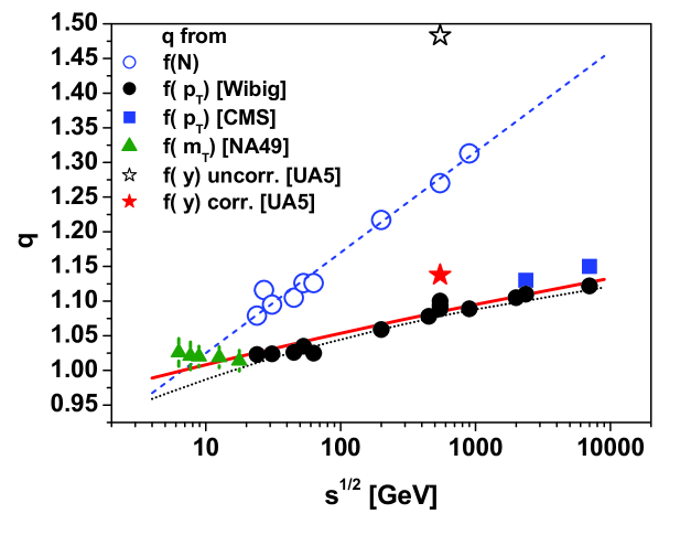
Figure 1: Examples of energy dependence of the nonextensivity parameter $q$ as obtained from different observables. Open symbols show $q$ obtained from multiplicity distributions $P(N)$ (fitted by $q=1+1/k$ with $1/k=-0.104+0.029\ln s$) [13]. Solid symbols show $q=q_{T}$ obtained from a different analysis of transverse momentum distributions, $f(p_{T})$. Data points are taken from, respectively, [14] for [Wibig], [8] for [CMS], from [15] for [NA49] (data on $\mu_{T}$) and from [16] for [UA5]. The dotted line represents a fit obtained in [14] (where $q_{T}=1.25-0.33s^{-0.054}$) and the full line comes from Eq. (8) (for $\rho=0$). Stars show $q=q_{L}$ obtained from $dN/dy$: open star taken from [16] (the same as used in [17]) shows the uncorrected $q$ value, whereas the solid star indicates its corrected value [10].

$$q-1=\left|\omega^{2}_{N}-\frac{1}{\langle N\rangle}\right|=\omega_{U}^{2}+\omega_{T}^{2}-2\rho\omega_{U}\omega_{T}.$$ (3)

What does the $\rho$ tell us? For example, a large energy $U$ (i.e., large inelasticity of reaction, $K$) can result either in a large number of secondaries of lower energies (for which $\rho<0$) or a smaller number of larger energies (for which $\rho>0$, different models give different predictions). Eq. (3) tells us that, in principle, the coefficient $\rho$ is a function of all the nonextensivity parameters involved. Let us then specify the part of fluctuations of $T$ which go in the transverse direction by $\alpha$, and write

$$q_{T}-1=\alpha\omega^{2}_{T},\qquad q_{L}-1=\omega^{2}_{U}+(1-\alpha)\omega^{2}_{T}.$$ (4)

From (4) one finds

$$\omega^{2}_{T}=\frac{1}{\alpha}\left(q_{T}-1\right),\qquad\omega^{2}_{U}=\left(q_{L}-1\right)-(1-\alpha)\omega^{2}_{T}=\left(q_{L}-1\right)-\frac{1-\alpha}{\alpha}\left(q_{T}-1\right).$$ (5)

Then, from (5) and (3) one gets

$$q-1=\left(q_{L}-1\right)+\left(q_{T}-1\right)-2\rho\omega_{U}\omega_{T}\qquad\stackrel{{\scriptstyle\rho\rightarrow 0}}{{\Longrightarrow}}\qquad q-1=\left(q_{L}-1\right)+\left(q_{T}-1\right).$$ (6)

Assuming that

$$\omega^{2}_{U}=\kappa^{2}\omega^{2}_{T},$$ (7)

Eq. (6) reads

$$q-1=\left(q_{L}-1\right)+\left(q_{T}-1\right)-2\rho\frac{\kappa}{\alpha}\left(q_{T}-1\right)$$ (8)

whereas from (7) and (5) one has that

$$\kappa=\frac{\omega_{U}}{\omega_{T}}=\sqrt{\alpha\left(\frac{q_{L}-1}{q_{T}-1}+1\right)-1}.$$ (9)

That results in a useful correlation coefficient given in terms of different (in principle measured) fluctuations:

$$\rho=\frac{1-\frac{(q-1)-\left(q_{L}-1\right)}{q_{T}-1}}{\frac{2}{\alpha}\sqrt{\alpha\left(\frac{q_{L}-1}{q_{T}-1}\right)-1}};\qquad\alpha=\frac{q_{T}-1}{\omega_{T}^{2}}.$$ (10)

Notice:

• to get the correlation coefficient $\rho$, one has to know all the fluctuations, i.e., both in the entire phase space, $q$, as separately in its transverse, $q_{T}$, and longitudinal, $q_{L}$, parts;

• out of them the best known is $q$ (no corrections needed);

• for $q_{T}$ the corrections are small and can be neglected;

• however, for $q_{L}$ the corrections are large and must be accounted for (cf., Fig. 1).

The example of feasibility of deducing $\rho$ from data is presented in Fig. 2 for data on $\bar{p}+p$ at $546$ GeV [16]. In this case from $P(N)$ one gets $q=1.27$, from distribution of $p_{T}$ one gets $q_{T}=1.09$ whereas from the original $q_{L}=1.48$ one gets after correction $q_{L}=1.14$ (cf. Fig. 1).

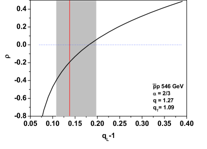
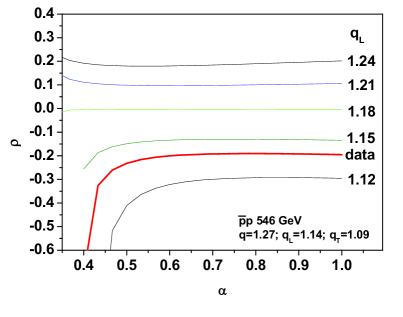
Figure 2: Left panel: the example of $\rho$ obtained from Eq. (10). The shaded area shows the extent of the possible error, due to uncertainty in fixing $q_{L}$. Right panel: the sensitivity of the correlation parameter $\rho$ to $\alpha$, specifying the fraction of fluctuations which goes into the transverse direction (in the case of full isotropy one has $\alpha=2/3$).

To summarize, one can say that it is a priori possible to obtain $\rho$ from experimental data, but - as shown here, this is difficult. Because of large estimation errors one cannot at this stage exclude the possibility that simply $\rho=0$. Our preliminary result, cautiously indicating that, perhaps, $\rho<0$, would prefer the production of a large number of particles of lower energies. However, statistically we cannot at this moment make a decisive statement.

3 Summary

We discuss the hadronization process where all variables characterizing an event, namely the energy $U$, temperature $T$ and multiplicity $N$ fluctuate. In this case, it follows that correlation $\rho$ between two of them (here chosen as $U$ and $T$), is necessary to fully describe the event. The question is: what is its meaning and can it be estimated experimentally? The answer to the first is that this parameter tells us how the available energy is used: either for production of particles or, rather, for making them more energetic. In what concerns the second, our preliminary result (indicating that, perhaps, $\rho<0$ ) would prefer the first scenario, however, statistically we cannot say so at the moment.

We conclude with two remarks. First, in what concerns Eq. (3), in the literature [18] there is similar relation connecting the volume, $V$, pressure, $P$ and temperature, $T$: $\omega^{2}_{P}=\omega^{2}_{V}+\omega^{2}_{T}$ [18]. Secondly, when all variables, $U$, $N$ and $T$ fluctuate, the pairs of variables, $(U,N)$ and $(U,T)$, cannot all be independent because

$$Var(U)=\langle T\rangle Cov(U,N)+\langle N\rangle Cov(U,T)$$ (11)

(cf., [11]). This means that, in general,

$$\omega_{U}=\rho(U,N)\omega_{N}+\rho(U,T)\omega_{T}.$$ (12)

where $\rho(X,Y)$ denotes the corresponding correlation coefficients between variables $X$ and $Y$ .

Acknowledgment: Partial support (GW) of the Ministry of Science and Higher Education under contract DPN/N97/CERN/2009 is gratefully acknowledged. We would like to warmly thank Dr Eryk Infeld for reading this manuscript.

References

- [1] M. Gaździcki, M. Gorenstein, P. Seyboth, Acta Phys. Polon. B 42, 307 (2011).
- [2] G. Wilk, Z. Włodarczyk, Eur. Phys. J. A 40, 299 (2009) and Central Europ. J. Phys., DOI:10.2478/s11534-011-0111-7 (in press, cf. also arXiv:1110.4220v2 [hep-ph]).
- [3] G. Wilk, Z. Włodarczyk, Phys. Rev. Lett. 84, 2770 2000) and Chaos, Solitons Fractals 13, 581 (2001).
- [4] T. S. Biró, A. Jakovác, Phys. Rev. Lett. 94, 132302 (2005); T. S. Biró, G. Purcel, K. Ürmösy, Eur. Phys. J. A 40, 325 (2009).
- [5] C. Beck, E. G. D. Cohen, Physica A 322, 267 (2003); F. Sattin, Eur. Phys. J. B 49, 219 (2006).
- [6] T. S. Biró, Is there a temperature? Conceptual Challenges at High Energy, Acceleration and Complexity, (Springer 2011).
- [7] A. Adare et al. (PHENIX Collaboration), Phys. Rev. D 83, 052004 (2011)
- [8] V. Khachatryan et al. (CMS Collaboration), JHEP02, 041 (2010), and Phys. Rev. Lett. 105, 022002 (2010).
- [9] C. Tsallis, Stat. Phys. 52, 479 (1988), Eur. Phys. J. A 40, 257 (2009) and Introduction to Nonextensive Statistical Mechanics (Springer, 2009).
- [10] G. Wilk, Z. Włodarczyk, W. Wolak, Acta Phys. Polon. B 42, 1277 (2011).
- [11] G. Wilk, Z. Włodarczyk, Physica A 390, 3566 (2011).
- [12] J. Lindhard, ’Complementarity’ between energy and temperature, in The Lesson of Quantum Theory, edited by J. de Boer, E. Dal, O. Ulfbeck (North-Holland, Amsterdam, 1986); J. Uffink, J. van Lith, Found. Phys. 29, 655 (1999);
- [13] A. K. Dash, B. M. Mohanty, J. Phys. G 37, 025102 (2010); see also C. Geich-Gimbel, Int. J.Mod. Phys. A 4, 1527 (1989).
- [14] T. Wibig, J. Phys. G 37, 115009 (2010).
- [15] C. Alt et al., Phys. Rev. C 77, 034906 (2008) and Phys. Rev. C 77, 024903 (2008); S. V. Afanasiev et al., Phys. Rev. C 66, 054902 (2002).
- [16] G. J. Alner et al. (UA5 Coll.), Z. Phys. C 33, 1 (1986).
- [17] M. Rybczyński, Z. Włodarczyk, G. Wilk, Nucl. Phys. B ( Proc. Suppl.) 122, 325 (2003); F. S. Navarra, O. V. Utyuzh, G. Wilk, Z. Włodarczyk, Phys. Rev. D 67, 114002 (2003).
- [18] Kulesh Chandra Kar, Phys. Rev. 21, 672 (1923).
- [19] M. Nauenberg, Phys. Rev. E 67, 036114 (2003); Phys. Rev. E 69, 038102 (2004); C. Tsallis, Phys. Rev. E 69, 038101 (2004); R. Balian, M. Nauenberg, Europhys. News 37, 9 (2006); R. Luzzi et al. Europhys. News 37, 11 (2006).
- [20] O. J .E. Maroney, Phys. Rev. E 80, 061141 (2009).
- [21] T. S. Biró, K. Ürmössy, Z. Schram, J. Phys. G 37, 094027 (2010); T. S. Biró, P. Ván, Phys. Rev. E 83, 061147 (2011); T. S. Biró, Z. Schram, EPJ Web of Conferences 13, 05004 (2011).