Analysis of power-law exponents by maximum-likelihood maps

Abstract

Maximum-likelihood exponent maps have been studied as a technique to increase the understanding and improve the fit of power-law exponents to experimental and numerical simulation data, especially when they exhibit both upper and lower cut-offs. The use of the technique is tested by analysing seismological data, acoustic emission data and avalanches in numerical simulations of the 3D-Random Field Ising model. In the different examples we discuss the nature of the deviations observed in the exponent maps and some relevant conclusions are drawn for the physics behind each phenomenon.

I Introduction

For the last few decades the study of critical phenomena has received a great deal of attention in many different areas of physics Sornette2000 . Criticality is often identified by the presence of statistical scale-free distributions of different magnitudes when a system evolves in time or when it is driven by an external force. The physical nature of the measured response can be very different: energy, displacement, magnetization, volume, polarization, resistivity, etc. In all cases, when the sudden changes (often called avalanches) of such magnitudes exhibit a statistical distribution compatible with a power law probability density function $g(x)dx\sim x^{-\alpha}dx$ one gains confidence about the existence of criticality. In some cases criticality has also been referred to as “crackling noise” Sethna2001 . At criticality the response of the system is characterized solely by the critical exponents $\alpha$. The theoretical understanding provided by the use of Renormalization Group techniquesBinney1992 states, in many cases, that critical exponents show a certain degree of universality. Thus, it has become extremely important to determine the values of $\alpha$ to a high degree of accuracy and confidence.

Within this framework, it is important to develop tools to test power-law behaviour of data samples and to fit critical exponents. The development of these statistical tools cannot be done without taking into account the limitations inherent to data acquisition. Typically in physics, data comes from experiment or computer simulation and in both cases one has boundaries to the proposed scale-free behaviour. These boundaries are not necessarily sharp or well defined. In experiments one finds unavoidable noise deforming the power-law distribution in the small-event region and different kinds of instrument saturation in the large-event region. One should take into account the fact that it is difficult to find instruments (amplifiers, voltmeters, etc.) that allow measurements with a range of more than 5 decades. In simulations one also finds unavoidable limitations: for instance, one has a minimum lattice parameter or particle size that alters the small-event distribution and finite-size effects deforming the large events. Since simulations with more than $10^{5}$ particles are scarce, it is also difficult to find power-law distributions extending many decades in numerical works. In addition, the existence of deformations in the region of small events is understood not only because of the reasons discussed above with a physical origin, but also because of a mathematical constraint: a pure power-law probability density with $\alpha>1$ cannot be normalized without a theoretical lower limit $x_{min}$.

It is easy to understand that a naked-eye analysis of standard histograms can be easily fooled, not only by the lack of statistics (insufficient data in the recorded sample), but also by the anomalies in the large- and small-event regions. The same may happen with traditional fitting methods such as the least-squares method (both linear and non-linear) which, for instance, depends on the binning process that is performed in order to plot the histograms.

Many years ago most of the community adopted the maximum-likelihood (ML) estimation methodGoldstein2004 ; Bauke2007 ; Clauset2009 as the safest way to treat data, although it is still frequent to see papers using alternative, error-prone fitting methods. Within this scenario, the work done by M.E.J. Newman and co-workers should be pointed out Clauset2009 . Using ML methods they have nicely illustrated how to test the power-law character of data and how to obtain good estimations (and error bars) of critical exponents. One of the proposed techniques consists of studying how robust the ML exponent is when the analysed data is restricted to being higher than an imposed lower cut-off $X_{low}$ that is varied by several decades. By this method one studies the deformation of the fitted exponent due to undesired effects in the region of small events.

In this paper we will study the extension of this technique to the analysis of the ML exponent as a function of both an imposed lower cut-off $X_{low}$ and an imposed higher cut-off $X_{high}$. This will render the so-called ML exponent maps Peters2010 . By this method we expect to be able to improve exponent estimation in the case in which experimental or simulation data presents distortions not only in the region of small events, but also in the large-event region.

In section II we will revisit the ML method and define ML exponent maps. We will include a discussion on numerical methods, evaluation of error bars and analysis of synthetic data obtained by pseudo-random number generation. In section III we will apply the proposed analysis technique to the study of three seismological catalogues from Japan, the San Andreas fault and the very recent activity in the island of El Hierro (Canary Islands). In section IV we will study three experimental cases corresponding to the measurement of the energy of acoustic emission (AE) events in different phenomena in solids, from previous literature The three sets of experiments have been carried out with the same experimental setup but with different experimental constraints (noise, amplification, etc..). The three cases correspond to (i) the compression of a porous material (Vycor) Salje2011 , (ii) a cubic-tetragonal structural transition in FePd Bonnot2008 and (iii) a cubic-monoclinic structural transition in a CuZnAl shape memory alloy Gallardo2010 . In Sec. V we will illustrate how to apply the technique to the study of numerical simulations of the 3D Random Field Ising model with metastable dynamics which is one of the prototypical frameworks for avalanche criticality Sethna1993 ; Perkovic1995 . Finally, in Sec. VI we will supply a summary and draw conclusions.

II Maximum-likelihood exponent map

Let us consider a sample of measurements $\{\mathrm{X}_{i}\}$ ($i=1,\cdots,N$) that we assume to be statistically independent. We will denote by capital letters $X_{max}$ and $X_{min}$ the smallest and the largest values in the sample set. Our aim is to model this set with a power-law probability density:

$$g(x)dx=\frac{x^{-\gamma}}{\zeta(\gamma)}dx\;\quad\;x_{min}<x<x_{max}$$ (1)

where $\gamma$ is the exponent that we wish to estimate and $\zeta(\gamma)$ denotes a normalization function. This normalization function will depend on $\gamma$ and the theoretical upper ($x_{max}$) and lower ($x_{min}$) bounds, as will be discussed below. (The case $x_{max}\rightarrow\infty$ is a particular case of our analysis). Note that these theoretical limits will not necessarily coincide with the maximum $X_{max}$ and minimum $X_{min}$ values in the sample. Nevertheless, given the power-law character of the probability density we expect that $X_{min}$ will be much closer to $x_{min}$ than $X_{max}$ to $x_{max}$. Table 1 clarifies the generic definitions of the limits and cut-offs that will be used within this section.

symbols	meaning
$x_{min}$, $x_{max}$	sharp bounds of the density $g(x)$
$X_{min}$, $X_{max}$	extreme values in the sample $\{X_{i}\}$
$X_{low}$, $X_{high}$	cut-offs imposed on the sample for the analysis

Table 1: Terminology used in this work to define the generic bounds and cut-offs used for the theoretical analysis in this section

The Likelihood function $\mathcal{L}$ is defined as the probability that the set of measurements $\{\mathrm{X}_{i}\}$ can be obtained by the proposed model:

$$\mathcal{L}(\gamma)=\prod_{i=1}^{N}g(\mathrm{X}_{i})$$ (2)

The Maximum Likelihood (ML) estimation method consists of choosing the value of $\gamma$ that maximizes the Likelihood Function, i.e. the value that makes the sample that we have obtained the most likely one to have occurred.

In order to evaluate the deviations of data with respect to the proposed model, in this work we will perform ML estimations by restricting the original data within the imposed lower cut-off $X_{low}$ and the imposed higher cut-off $X_{high}$, different from the theoretical limits $x_{min}$ and $x_{max}$ which are generally unknown. We will use the symbol $\hat{\gamma}$ to distinguish the exponent estimated within a restricted interval from the exponent estimated from the whole available sample. We will use $n$ ($n<N$) to denote the number of data of the restricted set. The normalization factor of the probability density with imposed cut-offs is:

$$\zeta(\hat{\gamma})=\int_{X_{low}}^{X_{high}}x^{-\hat{\gamma}}dx=\frac{X_{low}^{1-{\hat{\gamma}}}-X_{high}^{1-{\hat{\gamma}}}}{\hat{\gamma}-1}$$ (3)

The best estimation of $\hat{\gamma}$ is consequently found by maximizing the likelihood function:

$$0=\frac{\partial\ln\mathcal{L}(\hat{\gamma})}{\partial\hat{\gamma}}=-\sum_{\{X_{low}<X_{i}<X_{high}\}}^{n}\ln(\mathrm{X_{i}})-n\dfrac{\zeta^{\prime}(\hat{\gamma})}{\zeta(\hat{\gamma})}$$ (4)

where:

$$\dfrac{\zeta^{\prime}(\hat{\gamma})}{\zeta(\hat{\gamma})}=\dfrac{1}{1-\hat{\gamma}}-\dfrac{X_{high}^{1-\hat{\gamma}}\ln X_{high}-X_{low}^{1-\hat{\gamma}}\ln X_{low}}{X_{high}^{1-\hat{\gamma}}-X_{low}^{1-\hat{\gamma}}}$$ (5)

We should mention that for the case in which data is discrete (for instance, in many simulations of lattice models) the above treatment should be slightly modified. In this case, the data consists of the frequencies of occurrence $f(k)$ of a discrete set of values $\{k\}$ (which we will assume to be integers). We would like to fit it with a power-law probability function (called Zeta or Zipf)Goldstein2004 :

$$p(k)=\frac{k^{-\gamma}}{\zeta(\gamma)}\;\;k_{min}\leq k\leq k_{max}$$ (6)

Following the same procedure as above, when we restrict ourselves to data within imposed cut-offs $K_{low}$ and $K_{high}$, the normalization function is:

$$\zeta(\hat{\gamma})=\sum_{k=K_{low}}^{K_{high}}k^{-\hat{\gamma}}$$ (7)

and the derivative of the Likelihood Function will read:

$$\frac{\partial\ln\mathcal{L}}{\partial\hat{\gamma}}=-\sum_{\mathrm{k}=K_{low}}^{K_{high}}{f(\mathrm{k})\ln(\mathrm{k})+N\dfrac{\sum_{K_{low}}^{K_{high}}{\mathrm{k}}^{-\hat{\gamma}}\ln(\mathrm{k})}{\sum_{K_{low}}^{K_{high}}\mathrm{k}^{-\hat{\gamma}}}}$$ (8)

As opposed to what happens in the case in which one considers only a lower cut-off, equations (5) and (8) cannot be solved analytically. Thus, in this work, we will use the false position method in order to find roots Press1992 . This method generates a sequence of recursively smaller intervals that always include the root of the equation. The monotony of the derivative of $\ln\mathcal{L}$Miller2001 ensures that the false position method always converges to the root. We have chosen arbitrary starting values of $\hat{\gamma}_{1}=1$ and $\hat{\gamma}_{2}=3.5$, and have iterated the algorithm $M$-times until an interval $(\hat{\gamma}_{M-1},\hat{\gamma}_{M})$ is reached with a distance smaller than $0.005$.

By changing the $X_{low}$ and $X_{high}$ cut-offs we can plot the values of the ML estimations of $\tilde{\gamma}$ using a color scale and thus obtain the exponent map. Examples are shown in Fig. 1 and throughout the paper. Contour lines (in white) will also be shown separating exponent values in steps of 0.1. The maps exhibit a triangular shape since they are obviously limited by the condition $X_{high}>X_{low}$. The main goal of the map is to check the existence of a flat plateau (with an homogeneous color which is free of contour lines) in which the exponent is independent of the cut-offs and thus confirm the scale-free behaviour of the data. The map also allows anomalies to be identified that can have different origins, as will be discussed in the following sections by the use of examples.

One of the advantages of using the false position method for root finding is that we straightforwardly obtain an estimation of the second derivative of $\ln\mathcal{L}$ at the maximum:

$$\left.\frac{\partial^{2}\ln\mathcal{L}}{\partial\hat{\gamma}^{2}}\right|_{max}\sim\frac{\left.\frac{\partial\ln\mathcal{L}}{\partial\hat{\gamma}}\right|_{M}-\left.\frac{\partial\ln\mathcal{L}}{\partial\hat{\gamma}}\right|_{M-1}}{\hat{\gamma}_{M}-\hat{\gamma}_{M-1}}$$ (9)

Assuming Gaussian behaviour of the Likelihood Function (which is ensured by the Central Limit Theorem when $n$ is large enough) and under very general conditionsEadie , the second derivative provides us with an approximation to the standard deviation of the estimated exponent.

$$\sigma_{\hat{\gamma}}=\left[{-\left.\frac{\partial^{2}\ln\mathcal{L}}{\partial\hat{\gamma}^{2}}\right|_{max}}\right]^{-1/2}$$ (10)

It is easy to check that this expression, when $x_{max}\rightarrow\infty$, reduces to the equation proposed in Ref. Clauset2009, :

$$\sigma_{\hat{\gamma}}=\frac{\hat{\gamma}-1}{\sqrt{n}}$$ (11)

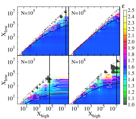
Figure 1: Exponent maps obtained from synthetic data. The data sets correspond to a theoretical probability density function with exponent $\gamma=1.55$ and bounds $x_{min}=1$ and $x_{max}=10^{8}$. The label $N$ indicates the size of the sample set. The two curved continuous lines indicate the limits above which the standard deviation becomes greater than 0.05. The red curved line corresponds to the estimation using Eq. (11) and the black curved line to Eq. (10). The vertical black straight line marks the highest value in the sample $X_{max}$

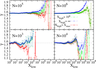
Figure 2: Comparison of the behaviour of the exponent fitted to synthetic data as a function of the lower cut-off $X_{low}$ when $X_{high}$ is fixed. Red squares correspond to $X_{high}=x_{max}=10^{8}$ (the theoretical limit of the synthetic data), green circles to $X_{high}=X_{max}$ (the maximum value found in the sample) and blue triangles to $X_{high}=\infty$.

As a first test of the usefulness of the ML exponent maps, we studied synthetic data Clauset2009 generated according to a power-law probability density with theoretical limits $x_{min}\leq x<x_{max}$:

$$g(x)dx=(\gamma-1)\frac{x^{-\gamma}}{x_{min}^{1-\gamma}-x_{max}^{1-\gamma}}dx$$ (12)

with $\gamma=1.55$, $x_{min}=1$ and $x_{max}=10^{8}$. The synthetic data samples were obtained using the RANECU generator James1990 for uniform random numbers in the $[0,1)$ interval and transformed using the method based on the inverse cumulative distribution function $F^{-1}(z)$. For the proposed probability density (12) the transformation function that converts uniform random numbers $z$ into the desired ones is given by:

$$x=F^{-1}(z)=\left[{x_{max}^{1-\gamma}-z(x_{max}^{1-\gamma}-x_{min}^{1-\gamma})}\right]^{\frac{1}{1-\gamma}}$$ (13)

Fig. 1 shows the resulting maps corresponding to four samples of increasing sizes $N$ as indicated by the legends. The first observation is that the size $N$ of the sample is crucial in order to obtain a clean plateau corresponding to the correct exponent. Only when $N\gtrsim 10^{4}$ does the plateau extend for several “square”-decades.

We have indicated the position of the maximum value $X_{max}$ obtained in the sample by a vertical black line. The variations of the fitted exponent observed from this line to the right are simply a consequence of changing the imposed upper cutoff $X_{high}$ in a region without available data due to the lack of statistics. This lack of data between $X_{max}$ and $X_{high}$ is relevant for the fitting method and, a priori, should be taken into account. Furthermore, the imposed cutoff $X_{high}$ can be moved above the theoretical limit $x_{max}$ or set to be $\infty$. This will then be equivalent to fitting the synthetic data (generated with a theoretical upper limit) with a model without such a limit. In the maps in Fig. 1 we have kept the imposed cut-off $X_{high}$ below the theoretical cutoff $x_{max}$, but note that for real data (e.g. in the following examples) this theoretical cut-off will be unknown.

Fig. 2 shows the behaviour of the fitted exponent $\hat{\gamma}$ as a function of the lower cut-off $X_{low}$ for the same synthetic data samples as in Fig. 1. We have compared three different ML estimations corresponding to three choices of $X_{high}$:

1. The green circles correspond to the ML estimation of the exponent obtained by fixing $X_{high}=x_{max}=10^{8}$ , the theoretical upper limit. This is nothing more than the profile of the ML exponent map along the vertical right border at $10^{8}$ in Fig. 1. This would be the correct way to perform the ML estimation if one could have a priori knowledge of the true upper cut-off.

2. The blue triangles (higher symbols) correspond to the ML estimation obtained by neglecting the existence of an upper limit in the power-law distribution, i.e. fixing $X_{high}=\infty$. This would precisely correspond to the method proposed by Ref. Clauset2009, .

3. The red squares (lower symbols) correspond to the ML estimation obtained by fixing the higher cut-off of the data to the maximum value found in the sample $X_{high}=X_{max}$. It corresponds to the profile of the map along the vertical black lines in Fig. 1.

For small $N$ Method 3 underestimates the exponent because it neglects the fact that no data has been observed between $X_{max}$ and $x_{max}$. However, for $N\gtrsim 10^{4}$, one can see that Method 3 renders exponents that are very similar to the correct ones (Method 1). For $N=10^{6}$ Method 3 is clearly better than Method 2, which neglects the existence of an upper boundary to the distribution: it can be seen that the two coinciding estimation methods (red squares and green circles) exhibit a larger plateau (by more than 1 decade) than the blue triangles.

It is also interesting to discuss the strong fluctuations of the ML exponent close to the diagonal of the maps, which can be observed in Fig. 1. These are due to the small size $n$ of the restricted sample set that increases the statistical fluctuations. We can locate the region where the standard deviation of the ML estimate is lower than $\pm 0.05$ Note1 by using the formulas (10) or (11) . These low-error regions correspond to the areas below the black- and red-curved lines, respectively. As can be seen, both estimations of the error differ, even in the region of small events. The estimation that takes into account the existence of both a low and a high cut-off obtained from Eq.(10) gives a better separation between the regions with meandering contour levels and the smooth, flat plateau.

To conclude this section, let us summarize what we have learned from the analysis of synthetic data: it does not make much sense to increase the higher cut-off $X_{high}$ above the maximum value in the data sample $X_{max}$ unless we have independent information of the theoretical limit $x_{max}$. Therefore, in the maps presented in the following sections we will scan the higher and lower cut-offs only within $X_{min}$ and $X_{max}$. Thus, the vertical right border of the maps will coincide with the vertical black line plotted in Fig. 1. In addition, we will use the error estimation proposed by equation (10) and plot, on the maps, the curved line separating the region with error bars greater than $\pm 0.05$ (above the line) from the region with lower error bars (below).

III Seismological catalogue analysis

The Gutenberg-Richter lawGutenberg1944 ; Utsu2002 describing the statistical distribution of earthquake magnitudes is one of the most famous examples of a scale-free phenomenon already discussed using ML methods in previous worksKagan1991 . Theoretical studies have proposed different physical models (Burridge-Knopoff Burridge1967 , Olami-Feder-Christensen Olami1992 , damage rheology Ben-Zion2009 ,…) and framework theories such as the so-called Self Organized Criticality Bak1987 ; Sornette1989 ; Main1996 which have explained, to a certain extent, the reasons behind this critical behaviour. It is not our purpose to gain any understanding of seismology, but only to use some of the available earthquake catalogues in order to test the behaviour of ML exponent maps.

Earthquakes are historically characterized by a quantity called magnitude $M$, which aims to be a logarithmic measure of the “size” or “energy released” during the earthquake. The Gutenberg-Richter lawGutenberg1944 refers to the number of earthquakes $N_{>}(M)$ with a magnitude larger than a certain value $M$ As a function of magnitude, the Gutenberg-Richter law can be written as:

$$N_{>}(M)\propto-bM$$ (14)

with $b\sim 1.0$. The measurement of earthquake magnitudes and energies is still a challenging issue for seismology. As the medium is too large to collect a significant amount of radiated energy, seismologists must rely on measurements of the sparse network of seismic stations in order to locate and estimate the “size” of an earthquake. Because of this, many different criteria are used, depending on the region, earthquake energy range, available instruments, etc. The catalogues usually contain mixed data corresponding to different definitions of the magnitude $M$. These definitions are not fully equivalent, especially for small earthquakesUtsu2002 ; Scordilis2006 . There are also different definitions of the “energy” associated with an earthquake (all of them are approximately linearly related): seismic moment, strain energy drop, radiated energy, etc.. In this work we will use a broadly accepted formulaHanks1979 that allows an approximate conversion of the different “magnitudes” $M$ to the minimum strain energy drop $E$ as:

$$\log_{10}E=1.5M+4.8$$ (15)

where $E$ is the energy in Joules. Using the Gutenberg-Richter law (14) and Eq. (15), one can write the probability density for earthquakes with energies between $E$ and $E+dE$ as:

$$p(E)dE\sim E^{-\epsilon}dE$$ (16)

where $\epsilon=1+(b/1.5)\simeq 1.67$ is the expected exponent characterizing the power-law distribution of earthquake energies.

We have computed the ML exponent maps corresponding to three earthquake catalogues:

1. The subduction process taking place in the Japan Trench makes it one of the most active seismological regions in the world. The area is quite well documented because of the vicinity of the Japanese islands. We studied the exponent map corresponding to the energy distribution for all the seismological events registered as earthquakes in the ANSSANSS catalogue from 2000/01/01,00:00:00 to 2011/11/09,17:32:36 within the region enclosed between latitudes 28^∘N and 48^∘N and longitudes 128^∘E and 148^∘E. The registered data correspond to the $N=14509$ events above $M=2.7$, where the the Tōhoku earthquake of 2011/03/11 was the most serious event with an estimated magnitude of $M=9.0$.

2. San Andreas fault systemOkubo1987 , beneath the region occupied by the states of California and Nevada, there is probably the most frequently monitored seismic region in the world and the best documented in catalogues. We will therefore take it as a precise example of a seismological strike-slip process. The data analysed here corresponds to the seismic signals registered as earthquakes in the ANSSANSS catalogue with its epicentre within the area of latitudes between 30^∘N and 42^∘N and longitudes between 114^∘W and 126^∘W during the period between 2000/01/01,00:00:00 and 2011/11/09,17:43:00. In order to avoid the presence of a possible noise background, we selected only those earthquakes with a magnitude greater than $M=0.4$. The strongest earthquake was recorded on 2005/06/15 off the Coast of Northern California with a magnitude of $M=7.2$. The data set has $N=453372$ events.

3. As a completely different seismological phenomenon (very localized in space and time), we considered the recent submarine volcanic eruption of La Restinga off the island of El Hierro (Canary Islands), which started in summer 2011. The volcanic activity triggered an earthquake swarmHainzl2003 which is expected to have quite different behaviour from typical tectonic processes. We considered the data obtained from the IGNIGN catalogue from 2011/06/08, 00:52:00 until 2012/2/07, 12:00:00 in the region enclosed by latitudes from 26.8^∘N to 27.6^∘N and longitudes from 17.85^∘W to 18.2^∘W. The data set has $N=12158$ events

The three ML exponent maps are shown in Fig. 3. We have kept the same scales in order to clearly reveal the different size $N$ of the statistical samples. Fig. 4 shows the behaviour of the fitted exponent $\epsilon$ as a function of the lower cutoff $E_{low}$ when the higher cut-off $E_{high}$ is fixed to the maximum value in the sample set, i.e. the profile of the map along the vertical right borders in Fig. 3.

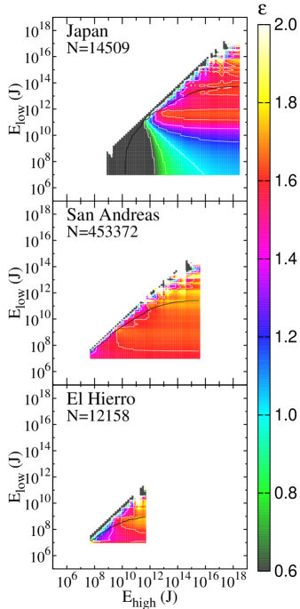
Figure 3: ML exponent map corresponding to the earthquake data from Japan, the San Andreas fault and El Hierro. White contour lines are separated by 0.1 units. The region above the black line corresponds to estimated statistical error bars greater than $\pm 0.05$.

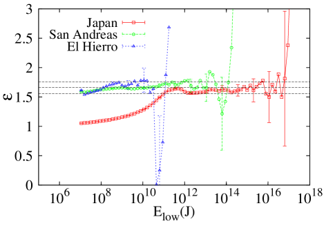
Figure 4: Behaviour of the ML exponent as a function of the lower cut-off $E_{low}$ for a fixed higher cut-off equal to the maximum value in the sample set. Only a few error bars are indicated. The horizontal dashed lines show the theoretically expected value 1.66 and an error bar $\pm 0.10$.

The first observation is that there is an almost perfect plateau exhibited by the San Andreas data (middle diagram) for a value close to the expected theoretical value $\epsilon=1.67$. Despite some deformation, indications of a plateau are also observed for the other two sets, Japan (top diagram) and El Hierro (bottom diagram). For the El Hierro data the coincidence is remarkable, given the different physical origins of the earthquake sequence.

A second important observation is the deformation of the plateau (towards low exponent values) for the Japan data in the region of $E_{low}<10^{10}J$. A plausible explanation for this deformation is that the statistics for small earthquakes in the Japan catalogue is incomplete. The same tendency can be observed for the San Andreas data, but for much lower minimum cut-offs $E_{low}<10^{8}J$, almost coinciding with the lower border of the map in Fig. 3 (middle diagram). The oscillation of the fitted exponent for the Japan data that can be seen on the maps (as contour lines with a parabolic horizontal shape starting from the right border) is also surprising as well as the maximum (about $E_{low}\sim 10^{11}-10^{12}J$) on the profile shown in Fig. 4. We are unable to provide an explanation for this behaviour, but it could be caused by the different methods used to estimate magnitudes and/or energies depending on the earthquake magnitude range.

IV Acoustic Emission Data Analysis

As a second set of experimental examples, we have focussed on much smaller energy scales. Different processes, which have been classified as critical or crackling noise, take place in solids, exhibiting a certain degree of disorder when driven by an external force or by a temperature ramp. Examples include superconductivityWu1995 , capillary condensationLilly1996 , acoustic emission in structural transitionsVives1994 ; Rosinberg2010 ; Planes2011 , Barkhausen noise in magnetismBarkhausen1919 ; Durin2006 , fractureRosti2009 , etc. In many cases, theoretical studies have provided general frameworks to understand the origin of this criticalityKardar1998 ; Fisher1998 ; Sethna2001 ; Zaiser2006 ; Alava2006 ; Perez-Reche2008 .

The following three experimental examples correspond to data recorded using the Acoustic Emission (AE) techniqueScruby1987 . Propagation of cracks or the sudden movement of internal interfaces generate acoustic waves in the ultrasonic range that propagate through the solid and that can be recorded by appropriate transducers on the surface. The AE method is equivalent to the method used to monitor earthquakes, but on a much smaller scale. It is interesting to describe here some details in order to understand the deviations that will be observed in the maps.

The most common piezoelectric transducers, coupled to the sample surface, generate a voltage signal $V(t)$ proportional to the speed of the incident elastic wave that is amplified. Using a predefined threshold (above the unavoidable experimental electrical and mechanical noise), it is possible to define individual AE events ManualPCI2 . The beginning of an event occurs at a time $t_{1}$ when the voltage exceeds the threshold. The end of the event occurs when the signal falls below the threshold at $t_{2}$ and remains below the threshold for more than a certain pre-defined time called the Hit Definition Time (HDT), typically in the range of 10-100 $\mu$s. The fast integration of the $V^{2}(t)$ signal from $t_{1}$ to $t_{2}$, normalized by a reference resistance, renders an estimation of the energy recorded by the transducer which is assumed to be proportional to the energy released by the physical process generating the elastic wave.

It is worth mentioning some experimental limitations of most standard set-ups: (i) acquisition systems, due to limited memory, have an internal maximum limit on the duration of a signal as well as a maximum limit on the voltage that saturates the amplifier. In the case that such maxima are exceeded, the signal is truncated both in voltage and/or duration. This represents a deformation in the large-event region and a not totally sharp cut-off in the measured energy since both voltage and duration can be independently exceeded. (ii) A second experimental problem that needs to be considered, is due to the attenuation of ultrasounds inside the material and the distance from the source of the AE event to the transducer. If the studied samples are small (compared to typical length scales for exponential attenuation or compared to typical transducer sizes) we expect that data recorded by a single transducer would not be very distorted by the distance to the source. However, if samples become large, the quality of the overall power-law distribution becomes poorer. One could then use several transducers to locate the position of the source of the event and correct for attenuation. This has been achieved in some cases Weiss2000 ; Vives2011 , thought, in general, it is a complicated procedure. The examples below correspond to the use of a single transducer. (iii)A third problem is that counting of the small signals is lower than expected for different reasons: an important fraction of signals that happen to be very short in time and/or amplitude cannot be detected by the acquisition set-up (they are too short for the sampling frequency or the amplitude is below the threshold value), or some of the small signals may be overlapped by the tails of previous signals due to dead-time HDT.

In the cases analysed in the following three subsections, the same experimental set-up for the acquisition of AE has been used: a PCI2-system from the MISTRAS Group, which consists of an 18-bit A/D converter working at a base sampling rate of 40 MHz. The transducers are also the same in the three examples (micro80). This makes the ML exponent maps easy to compare. The amplification factor, the threshold and the number of recorded signals used in each case are different, given the different noise conditions and differing nature of the studied phenomenon and driving force. Although the acquisition card is only 18 bits ($\sim 5$ decades), the measured energies by the fast integration algorithm may theoretically extend many more decades. In order to compare the different studies, we will keep the same scales: from $10^{-17}$J to $10^{-9}$ J for energy and from 1.0 to 2.5 for the fitted exponent $\epsilon$.

IV.1 Mesoporous SiO₂ under compression

The study of noise in porous materials under compression is important for the prediction of accidents in mining. In this first exampleSalje2011 two samples of a porous material SiO₂ (Vycor) with two parallel faces are compressed between two plates with a lineally increasing load in time. The AE sensor is attached to one of the plates. There are two sets of data studied corresponding to the AE events recorded at two loading rates: 0.2 kPa/s and 1.6 kPa/s. The study of the influence of the driving rate is important because, in some cases, it affects the fitted exponents due to the overlap of large and small avalanchesDahmen2003 ; Perez-Reche2004c . The material cracks under compression and the recorded AE signals show a power-law distribution of energies. In this case a preamplifier of 60 dB was used and the threshold was selected to be 26dB. The number of recorded signals was $N=11022$ and $N=28652$ for the first and second set, respectively.

Fig. 5 shows the ML exponent maps obtained with the two driving rates. It is clear that, in both cases, there is a vast region of the map with a constant plateau corresponding to a common value of the exponent close to 1.4. This means that the exponent is robust against changes in the cut-offs by several decades. The small coloured spots observed close to the diagonal of the map as well as the large peak in the upper right-hand corner correspond to expected statistical fluctuations, above the black line that indicates when the statistical error bar becomes larger than $\pm 0.05$. The black region in the bottom left-hand corner corresponds to the fact that the exponent decreases when only an important fraction of very low signals is included in the analysis which gives an erroneous estimation for the reasons explained above. Basically, no other deviations are observed in this example.

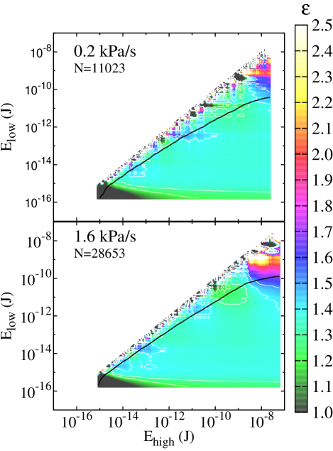
Figure 5: ML exponent maps corresponding to the AE recorded during the compression of Vycor samples at two different rates, 1.6kPa/s (above) and 0.2 kPa/s (below). White lines correspond to the exponent contour levels with a separation of 0.1. The region above the black line indicates an estimated error bar grater than $\pm 0.05$.

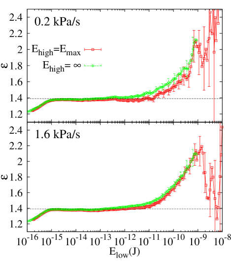
Figure 6: Profiles along the right vertical border of the exponent maps corresponding to the Vycor experiments, compared to the profiles proposed in Ref. Clauset2009, . Some typical estimated error bars are shown. The horizontal line indicates the value $\epsilon=1.39$ proposed in Ref. Salje2011, .

Fig. 6 shows the analysis of the profiles of the map along the right vertical border ($E_{high}=E_{max}$) compared to the analysis proposed in Ref. Clauset2009, assuming no upper limit for the power-law distribution ($E_{high}=\infty$). As can be observed, the two profiles are similar, but are not identical. They show a clean plateau at $1.39\pm 0.02$ for three decades ($10^{-15}-10^{-12}$). The profile obtained by fixing the highest cut-off to the maximum value in the sample (i.e. along the right-hand border of the ML exponent map in Fig. 5) shows flatter behaviour along, at least, one more decade.

Therefore, one can conclude that this example shows a very robust power-law behaviour, comparable to that observed for seismological data.

IV.2 Structural transition in FePd

In this second case we present an analysis of the AE recorded during a martensitic transition in Fe-Pd Bonnot2008 . This alloy has received a lot of theoretical interest due to the simple symmetry relation between the high-temperature phase (cubic) and the low-temperature phase (tetragonal). The transition can be induced by applying an external stress or by changing temperature. Two samples were considered in the study: a single crystal and a polycrystal with the same composition Fe_68.8Pd_31.2. The transition was induced by changing the temperature at different driving rates between 0.1K/min and 10K/min. Apart from the critical distribution of energies during the events, the AE study revealed other interesting features (which were not found by other techniques). The transition, on cooling, started at the same temperature $M_{s}=246\pm 2K$ for the two samples. As soon as the transition started the formation of new tetragonal domains or the advance of interfaces separating previously nucleated domains, generated AE events. Due to the thermoelastic behaviourOrtin1989 of the transition the AE extended for many degrees ($\sim 35K$) until the sample was fully transformed. On heating, the reverse process occurred with low thermal hysteresis ($\sim 1$K).

In this case AE was amplified $60$dB and the threshold was chosen to be 22dB. The four sets of data that we will analyze here correspond to a driving rate of $1K/min$ for both the single crystal and the polycristal and for cooling and heating runs. In order to increase statistics, data were accumulated over 20 ramps. This accumulation technique would correspond to a real increase of the statistics only if the data recorded on each ramp is independent of the previous data. This assumption is doubtful in the case of structural transitions since it has been demonstrated that samples exhibit a learning process that increases the correlation of the signals between consecutive ramps Perez-Reche2004b . In this case the ramps corresponding to the same driving rate were not strictly consecutive since other driving rates were added in between, thus the independence of the recorded data is not clear.

The total number of recorded signals was $N=171056$ (single crystal, cooling), $N=111840$ (single crystal heating), $N=192596$ (polycrystal cooling) and $N=58501$ (polycrystal heating). Typically, the number of AE events is not symmetric during heating and cooling ramps and there is a lack of understanding of this phenomenonVives1994 .

The study Bonnot2008 concluded that in the four cases the energies of the individual AE events were power-law distributed ( $\sim 4$ decades for the single crystal and $\sim 3$ decades for the polycrystal). The exponents were fitted using the ML method and were almost independent of the heating/cooling rate. The values of the cut-offs were selected in the region where the statistics were sufficiently high. For the single crystal both cooling and heating ramps exhibited an exponent compatible with a value of $1.64\pm 0.10$. For the polycrystal a clear deviation of the exponent was found when the heating ($2.0\pm 0.1$) and cooling ramp ($1.59\pm 0.10$) were found. So far, we have no explanation for this deviation.

Fig. 7 and  8 show the ML exponent maps corresponding to the four cases. The graphs above correspond to cooling data and the graphs below to heating data. As can be observed the coloured spots attached to the diagonal, which correspond to statistical fluctuations are larger (in absolute terms) than in the previous example. This suggests that, although the recorded number of signals is $\sim 10$ times larger, most probably data corresponding to the different 20 runs were correlated and did not effectively increase the statistics. Thus, the estimated error bars were, most probably, underestimated by a factor of $\sqrt{20}$. Therefore, in order to plot the curved black line on the map separating the zone with large error bars, we have required that $\sqrt{20}\sigma_{\hat{\gamma}}=0.05$. It can be seen that, indeed, the curved line separates the zone with fluctuating contour lines from the flat region. By observing the map corresponding to the heating runs (Fig. 8 bottom) for the polycrystalline sample one clearly sees that the large fitted exponent $\sim 2.0$ is doubtful and most probably is a consequence of the lack of statistics. The region with small enough error bars (below the black line) is very small and it is difficult to identify any plateau. For the cooling ramps (Fig. 8 top) the plateau is not very clear but at least the separation of the contour lines is much wider.

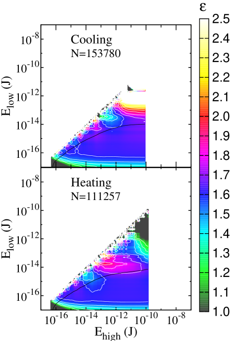
Figure 7: Exponent maps for AE in the FePd single crystal corresponding to heating ramps (below) and cooling ramps (above). The region above the black line corresponds to estimated error bars greater than $\pm 0.05$, after correcting by a factor of $\sqrt{20}$ due to the possible correlations between measurements (see text). The contour lines (in white) are separated by 0.1 units.

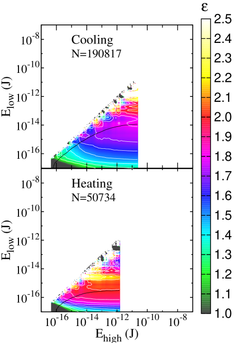
Figure 8: Exponent maps for AE in the FePd polycrystal corresponding to heating ramps (below) and cooling ramps (above). The region above the black line corresponds to estimated error bars above 0.05, after correcting by a factor of $\sqrt{20}$ due to the possible correlations between measurements (see text). The contour lines (in white) are separated by 0.1 units.

Fig. 9 shows the corresponding profiles along the right vertical border of the map. Error bars have been increased by a factor of $\sqrt{20}$ compared to the ones reported in the original paper Bonnot2008 . The dashed lines indicate the proposed exponent $1.64\pm 0.1$. The hypothesis that this might be a common value for the exponent corresponding to the four cases cannot be ruled out due to the lack of statistics. More measurements for the polycrystalline sample would be required to fully clarify this point.

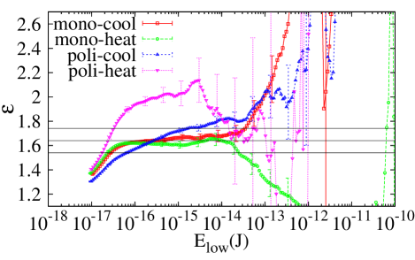
Figure 9: Exponent values versus lower cut-off $E_{low}$ for AE in FePd. The horizontal lines show the value $1.64\pm 0.10$ proposed in Ref. Bonnot2008

IV.3 Structural transition in CuZnAl

This third example corresponds to a recent study of AE during the martensitic transition in a CuZnAl shape-memory alloy Gallardo2010 . In this case the transition is also thermally induced from a monoclinic multivariant structure at low temperatures to a cubic structure at high temperatures. The purpose of the analysis performed in Ref. Gallardo2010, was not to demonstrate the power-law distribution of the AE events (which had been shown previously in different studies Vives1995 ; Carrillo1998 ), but to compare the observed exponent with the exponent corresponding to the very large avalanches that can also be recorded by a sophisticated calorimetric study. The sample studied was, therefore, larger than those studied previously. This, as explained above may lead to distortion of the power law. Furthermore, a larger sample typically requires a more powerful temperature control set-up, involving higher electric currents and thus involving greater noise. Since the study was focussed on large avalanches and noise was high, the amplification was set to a much lower factor, 40 dB, and the threshold to 45 dB. The data set analyzed consists of $N=17936$ signals corresponding to a unique heating ramp.

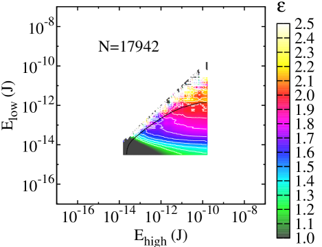
Figure 10: ML Exponent map corresponding to the martensitic transition in a CuZnAl sample during a heating ramp.

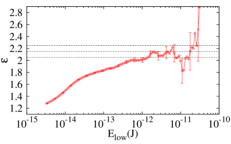
Figure 11: ML fitted exponent as a function of the lower cutoff $E_{low}$ when considering a higher cut-off equal to the maximum recorded signal in the data sample. The horizontal lines indicate the value $2.15\pm 0.10$.

As can be seen in Fig. 10, the exponent map shows a poorer quality without any clear plateau. The profile shown in Fig. 11, corresponding to the right vertical border of the map, suggests an incipient plateau around $\epsilon=2$ for slightly more than one decade, but this is not fully conclusive. Thus, the exponent map analysis in this case indicates that either the number of signals is too small to draw conclusions about the power-law behaviour of the data or the distribution shows a deformation probably due to the fact that the sample was too large and attenuation introduces a length scale. Note, however, that we are not fully compromising the results pointed out Ref. Gallardo2010, . The conclusions were based not only on AE signals, but also on the coincidence of the observed incipient plateau at $\epsilon=2$ with the plateau observed by a different experimental technique.

V Simulation data

As a last case we will analyze data corresponding to numerical simulation of a lattice model. This is an interesting illustrative case of the advantages of ML maps compared to the previous proposed analysis assuming no upper limit. This is because the distortions affecting the large avalanche region are not due to measurement problems, but are intrinsic to the finite size of the model. The study corresponds to the 3D Gaussian Random Field Ising Model (3D-GRFIM) driven by an external field $H(t)$ with metastable dynamics at zero temperature Sethna1993 . The model is based on the original Ising model with the addition of random internal fields $h_{i}$ acting on each spin $S_{i}=\pm 1$. The values $h_{i}$ are quenched and distributed according to a Gaussian probability density $\rho(h)dh=\frac{1}{\sqrt{2\pi}R}e^{\frac{-h^{2}}{2R^{2}}}dh$ with zero mean and variance $R^{2}$. The parameter $R$ is usually referred to as the amount of disorder in the system. The Hamiltonian of the system reads:

$$\mathcal{H}=-\sum_{\langle i,j\rangle}S_{i}S_{j}-\sum_{i}^{N}h_{i}S_{i}-H(t)\sum_{i}^{N}S_{i}$$ (17)

where the $S_{i}$ spin variables are defined on a regular cubic lattice and the first sum extends over all nearest-neighbour pairs. The simulations of the model start from a saturated configuration $\{S_{i}\}=-1$ and $H=-\infty$ . The field is then adiabatically increased and the spins flip according to the local relaxation rule:

$$S_{i}=sign\left(\sum_{j}S_{j}+h_{i}+H(t)\right)$$ (18)

where the sum extends over all the $z=6$ neighbours of the spin $S_{i}$. With this metastable dynamics the system evolves following a sequence of magnetization jumps (avalanches) occurring at certain fixed values of the external field separated by periods of inactivity in which the field is increased without producing any spin flip.

The model has been widely used as a prototype model for the study of avalanche dynamics. It has been successful in explaining different features of the magnetization process in ferromagnets: the presence of rate independent hysteresis, the return point memory property and the existence of Barkhausen noise Sethna1993 . Extensions of the model have been also used for the understanding of other athermal first-order phase transitions.Vives2001 ; Cerruti2008

Here we will focus our attention on the distribution $D(s,R)$ of the sizes $s$ (number of flipped spins) of the avalanches obtained along the magnetization process from $H=-\infty$ to $H=+\infty$, i.e. the so-called integrated distribution. In the thermodynamic limit and when the amount of disorder $R$ is tuned to the critical value $R_{c}$, this distribution is expected to be a power lawSethna1993 ; Perkovic1999 ; Perez-Reche2003 ; Perez-Reche2004 characterized by a critical exponent called $\tau^{\prime}=\tau+\sigma\beta\delta$

$$D(s,R_{c})=\frac{s^{-\tau^{\prime}}}{\sum_{s=1}^{\infty}s^{-\tau^{\prime}}}$$ (19)

For values of disorder above $R_{c}$ it is expected that the distribution of avalanche sizes is exponentially damped and thus, in the thermodynamic limit, the discontinuities in the magnetization $\Delta m=s/L^{3}$ vanish. Below $R_{c}$, it is expected that the distribution of avalanches is also exponentially damped, but there will exist a unique massive avalanche with a size proportional to $L^{3}$ that is responsible for a magnetization discontinuity as should occur given the first-order character of the phase transition.

In the numerical simulations on a finite lattice ($L\times L\times L$) with periodic boundary conditions, nevertheless, the distribution of avalanche sizes $D(s,R,L)$ behaves quite differently. Several effects deform the power-law character at the “pseudo”-critical point:

On the one hand, avalanche sizes are limited from above by the finite size $s<L^{3}$. The fact that in all critical phenomena with an associated diverging correlation length, distortions occur well below the limit $L^{3}$ is well known. Among other reasons, close to the critical point $R_{c}$, the avalanches are expected to be fractal Perkovic1995 ; Perez-Reche2004 and thus exceed the lattice side $L$ when its size is much smaller than $L^{3}$. Such avalanches that expand the lattice side $L$ in, at least, one dimension, are the so-called spanning avalanches. For a cubic lattice with periodic boundary conditions, they can be easily classified as 1D-spanning, 2D-spanning or 3D-spanning depending on whether they span the lattice side in 1,2 or 3 spatial dimensions.

On the other hand, some small avalanches (sometimes called lattice animals within percolation theory Stauffer1994 ) may occur for probabilistic reasons even very far away from the critical point. For any value of $R$ and $H$ it is possible to compute the probability that two neighbouring spins (surrounded by negative spins) flip simultaneously. The same computation can be carried out for the probability of a group of three, four, etc. neighbouring spins with a certain topological configuration to flip simultaneously. It is clear that in such a computation the number of configurations in which spin clusters (lattice animals) with a certain size $s$ can be constructed plays a fundamental role. Such a phenomenon has (a priori) no connection with the critical point. The total number of such non-critical avalanches is, nevertheless very large (it increases with $L^{3}$) and renders a distribution of small avalanches that has general, fast decreasing behaviour with $s$, but is non-monotonous. At the critical point this effect overlaps with the proposed power-law distribution and thus shows a deformation in the small-size region of the distribution $D(s;R,L)$, which typically can be observed below $s\sim 10$. Our goal here is to show how these distortions at large and small sizes show up on the ML exponent map.

Before the discussion of our results, it is important to recall that the exact values of $R_{c}$ and $\tau^{\prime}$ have not been definitely established. The problems are precisely due to the fact that it is difficult to deal with spanning avalanches in the simulations on a finite lattice. There have been two main approaches:

1. Dahmen and coworkers found $R_{c}=2.16\pm 0.03$ and $\tau^{\prime}=2.03\pm 0.03$ by performing a scaling collapse of the avalanche distribution, neglecting the fact that there should be a dependence on $L$ in the distribution. This was first done Perkovic1999 on very large systems (up to $1000^{3}$) but averages over very few realizations of disorder. The collapses clearly revealed that corrections to scaling were needed. LaterLiu2009 similar collapses were done which included a unique system size $64^{3}$. In both cases, the data were restricted to amounts of disorder $2.25<R<6.0$ well above $R_{c}$. By this method they avoided most spanning avalanches in the simulations but paid the price of working too far from the critical point and so they had to extrapolate the value for the exponent.

2. Furthermore, there have been studies precisely focussed on the behaviour of spanning avalanches which analyse how they concentrate close to the critical pointPerez-Reche2003 ; Perez-Reche2004 . Such studies have performed finite-size scaling analysis of the number of spanning avalanches and have obtained a higher value of the critical amount of disorder $R_{c}=2.21$. To do so, they proposed a method (called method-2 in Ref. Perez-Reche2004, ) to separate the 3D-spanning avalanches that will correspond to the massive avalanches that clearly disturb the power-law distribution of avalanche sizes in the region of large events, close to the critical point. Such 3D-spanning avalanches are identified when they are the unique spanning avalanches in the full-field excursion. This allows them to be filtered from the statistical analysis. The reason behind the separation method is that when massive avalanches occur, they fill such a large fraction of the system that they do not allow for any other spanning avalanche to take place. It was shown that this filtering method, although not perfect, gave more consistent results in the finite-size scaling analysis than the method of discarding all the spanning avalanches.

The differences between the two above approaches are even more subtle and difficult to summarize here. Let us simply remark that the two analysis use a slightly different scaling variable to measure the distance to the critical point and that the exponent $\tau^{\prime}=2.03\pm 0.03$ proposed in Ref. Perkovic1999, is interpreted not as a true critical exponent, but as an effective exponent $\tau^{\prime}_{eff}$ in Ref. Perez-Reche2003, . Instead, they propose that close to the critical point the distribution of avalanche sizes (neglecting the massive avalanches) will be dominated by non-critical lattice animals (in the small s region) and by the so-called non-spanning critical avalanches (in the intermediate and large s region). Only the last kind of avalanches may exhibit true power-law behaviour with an exponent $\tau_{nsc}=1.65$ at $R_{c}=2.21$.

We have performed numerical simulations with system sizes ranging from $L=32$ to $L=256$ and values of $R$ within the range $2.15<R<2.24$. For every size $L$ and every $R$, averages were taken over 2000 configurations of the random fields for $L\leq 128$ and over 1400 for $L=256$. We used the RANECU random number generator and a Box Muller-Polar Marsaglia algorithm to generate the Gaussian random fields. Simulations of the metastable dynamics were done with the sorted list algorithm Kuntz1999 . The typical sizes of the sample sets of recorded avalanches (corresponding to each single value of $R$) range from $10^{6}$ for $L=32$ to $10^{9}$ for $L=256$.

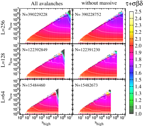
Figure 12: ML exponent maps corresponding to the 3D-GRFIM for $R=2.20$ and increasing system sizes from $L=64$(below) to $L=256$ above. The left-hand column shows the maps that where obtained by considering all the recorded avalanches, whereas the right-hand column, the method proposed in Ref. Perez-Reche2004, was used to suppress the massive, large non-critical avalanches. The region above the black line (very close to the diagonal of the map) corresponds to an estimated error bar of $\pm 0.05$. Contour lines in white are separated by 0.1 units

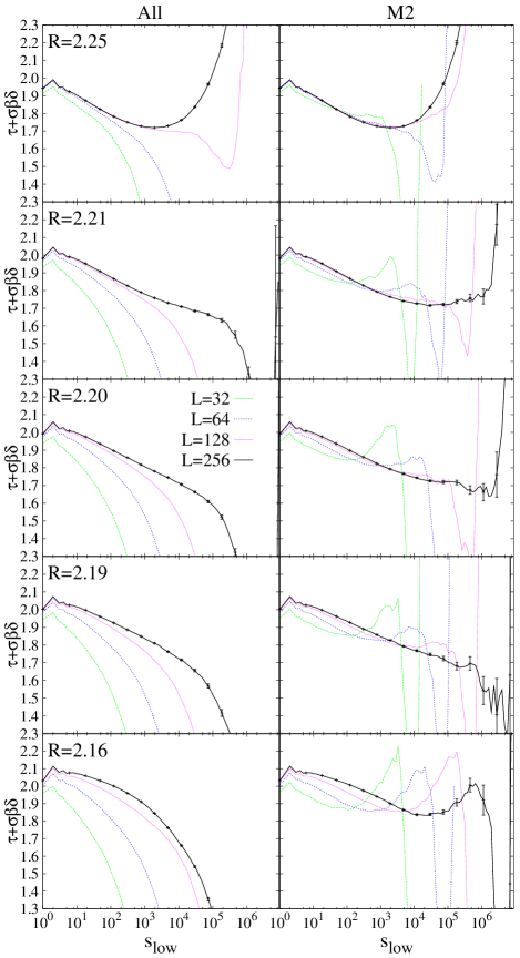
Figure 13: Profiles of the ML exponent maps along the vertical right border for different values of $R$ and $L$. Data in the left column corresponds to the full set of avalanches. On the right column data corresponds to the same sets after filtering the massive avalanches following the method proposed in Ref. Perez-Reche2004, .

Fig. 12 shows the exponent maps corresponding to $R=2.20$ and increasing values of $L$. The first column corresponds to the exponent obtained by considering all the avalanches and the second column to the analysis after the suppression of the massive avalanches, as explained in Ref. Perez-Reche2004, . As can be observed in the first column the maps display an approximately triangular black region in the upper right-hand corner that also extends along the right edge which is due to including of such “massive” avalanches that they strongly distort the possible power-law distribution. Massive avalanches overpopulate the large $s$ region and thus decrease the value of the fitted exponent. Such a deformation disappears when the data is filtered, as can be seen in the right column in Fig. 12.

Close to the bottom horizontal boundary of the maps, exponent oscillations (seen as a sequence of parallel horizontal contour lines) can also be observed in all the graphs. These oscillations are due to non-critical avalanches (lattice animals) which are always present and difficult to subtract.

Besides these two observed deformation regions, it is not clear that a clean plateau exists close to the bottom right-hand corner, with an area increasing with $L$. The maps show a slow decrease of the exponent from $2.1$ towards $1.7$ when increasing the lower cutoff $s_{low}$, and this effect does not seem to disappear for large system sizes. Instead, a region with a value of the exponent close to $1.6-1.7$ seems to develop close to the upper corner when the system size is increased up to $L=256$. This effect is clearer when the data has been filtered (right column) and suggests that a true power law may only be observed when small avalanches are not included in the analysis.

Fig. 13 shows the profiles of the maps obtained by fixing $s_{high}=s_{max}$, for different values of $R$ between $2.16$ and $2.25$ and $L$ from $32$ to $256$. The column on the left corresponds to the analysis of all the avalanches and the column on the right to the analysis after filtering the massive avalanches. Again, it is difficult to find any clear evidence of a plateau growing with $L$. The only exception seems to be for $R=2.20-2.21$ in the region of intermediate and large cut-offs ($10^{4}<s_{low}<10^{6}$), where a plateau seems to form and become broader when $L$ increases. This plateau has a height approaching $\tau^{\prime}\simeq 1.7$. It can be observed not only on the filtered data (right column), but also as an inflection when the avalanches are not filtered (left column).

The profiles in Fig. 13 also allow the oscillations in the small avalanche region ($s_{low}<20$) to be observed. The peaks in the exponent correspond to even sizes. This indicates that small avalanches with odd sizes occur with a higher frequency than the frequency corresponding to a perfect power law.

Note also that for the critical value $R_{c}=2.16$ proposed in Ref. Perkovic1999, , the possible plateau at a height $\tau^{\prime}\sim 2.03$ does not exhibit a clear tendency to increase with $L$: it is very much distorted by odd-even fluctuations and, already for $s_{low}=10^{2}$, has clearly decreased for all the studied system sizes.

In our opinion, a final understanding of the behaviour of these distributions can only be achieved after a full finite-size scaling analysis of the distribution $D(s;R,L)$ (involving the three variables), which is beyond the scope of this paper. Nevertheless, in view of the above observations it seems that the distribution of avalanche sizes at the critical point shows two contributions: (i) the actual power-law behaviour corresponding to the non-spanning critical avalanches with $\tau^{\prime}\simeq 1.7$ that can only be observed at intermediate and large avalanche sizes, and (ii) the contribution from non-critical avalanches (lattice animals), in the small $s$ region, which distorts the exponent towards the effective value $\tau^{\prime}_{eff}\simeq 2.03$. This scenario is not incompatible with previous numerical studies.

VI Summary and conclusions

The aim of this paper has been to illustrate the usefulness of ML exponent maps in order to study distortions of power-law behaviour to the critical distributions of events. Such distortions are expected to occur for most experimental and numerical simulation data due to different reasons. Fig. 14 shows a schematic representation of the main conclusions of this paper. On the left we show the ML exponent map that one can expect for experimental data. When the sample set is small, a lack of statistics creates deformations of the theoretical plateau close to the diagonal axis of the map, which can be bounded by a proper estimation of the statistical error bars. Noise and undercounting of small-size events renders a deformation region starting in the bottom left-hand corner and which extends horizontally along the bottom border. Saturation of the amplifiers and counters also deforms the plateau in the upper right-hand corner and along the right edge. Between these three boundaries there should be a region with a well-defined plateau. The black dot indicates the best values of the high and low cut-off for the determination of the critical exponent. It should be mentioned that, if the size of the sample set is too small, such an ideal situation might not be achieved.

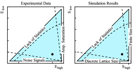
Figure 14: Schematic representation of ML exponent maps for experimental data (left) and simulation data (right). The lines indicate the regions where we can expect deformations of the theoretical plateau. The dot indicates the best values of the cut-offs for the estimation of the exponent.

The right plot shows a similar scheme for numerical simulations of lattice systems. The deformation regions are similar to the previous ones. Along the bottom edge we find the footprint of the lattice character of the model that deforms the perfect power-law behaviour. Along the vertical right edge we find deformations associated with finite-size effects, which in some cases can be partially corrected.

The examples analyzed in this work have included: three seismological catalogues corresponding to Japan, the San Andreas fault and El Hierro volcanic activity, three sets of Acoustic Emission data corresponding to the fracture of Vycor under compression, a cubic-tetragonal structural transition in FePd and a cubic-monoclinic structural transition in CuZnAl and, finally, numerical simulations of the 3D Random Field Ising model. These three case studies of the maps have allowed the good quality of the data to be checked or hypothesis for the observed distortions to be proposed. The studies have also been used to suggest improvements to measurements and/or numerical simulations.

- (1) D.Sornette, Critical Phenomena in Natural Sciences, Springer Series in Synergetics, Springer Verlag (Berlin Heildelberg 2000).
- (2) J.P.Sethna, K.A.Dahmen and C.R.Myers, Nature 410, 242-250 (2001).
- (3) J.J.Binney, N.J.Dowrick, A.J.Fisher and M.E.J.Newman, The theory of critical phenomena, Oxford Science Publications, Clarendon Press (Oxford 1992).
- (4) M.L. Goldstein, S.A. Morris and G.G.Yen, Eur. Phys. Journ. B 41, 255-258 (2004).
- (5) H. Bauke, Eur. Phys. Journ. B 58 167-173 (2007).
- (6) A.Clauset, C.R.Shalizi, M.E.J.Newman, SIAM Review 51661-703 (2009).
- (7) O. Peters, A.Deluca, A.Corral, J.D.Neelin and C.E.Holloway, J. Stat. Mech., P1103 (2010).
- (8) Ekhard K.H. Salje et al., Phil. Mag. Lett.91, 554-560(2011).
- (9) E.Bonnot et al, Phys. Rev. B 78, 184103 (2008).
- (10) M.C.Gallardo et al, Phys. Rev. B 81, 174102 (2010).
- (11) James P. Sethna, Karin Dahmen, Sivan Kartha, James A. Krumhansl, Bruce W. Roberts, and Joel D. Shore, Phys. Rev. Lett. 70, 3347 (1993).
- (12) Olga Perkovic, Karin Dahmen, and James P. Sethna, Phys. Rev. Lett. 75, 4528 (1995).
- (13) W.H.Press, S.A.Teukolsky, W.T.Vetterling and B.P.Flannery, Numerical Recipes in FORTRAN, 2nd ed., Cambridge University Press (1992).
- (14) K. S. Miller S. G. Samko Integr. Transf. and Spec. Funct. 12, 4, 389-402 (2001).
- (15) W. T. Eadie,Frederick James Statistical Methods in Experimental Physics North-Holland Publishing Co. (1971).
- (16) F. James, Comp. Phys. Comm. 60, 329 (1990).
- (17) This precise value has been chosen because the contour lines of the map, in white, are plotted in steps of 0.1.
- (18) B. Gutenberg and C. F. Richter, Bull. Seismol. Soc. Am. 34, 185 (1944).
- (19) Tokuji Utsu, International Geophysics 81 Part A, 733 (2002).
- (20) Y. Y. Kagan, Geophys. J. Int. 106, 135 (1991).
- (21) R. Burridge and L. Knopoff, Bull. Seismol. Soc. Am. 57, 341 (1967).
- (22) Z.Olami, H.J.S.Feder, and K.Christensen, Phys. Rev. Lett. 68, 1244 (1992).
- (23) Yehuda Ben-Zion and Jean-Paul Ampuero, Geophys. J. Int. 178, 1351 (2009).
- (24) P. Bak, C. Tang and K. Wiesenfeld, Phys. Rev. Lett.59, 381 (1987).
- (25) A. Sornette, D. Sornette, Europhys. Lett. 9, 197 (1989).
- (26) I. Main, R. Geophys. 34,433 (1996).
- (27) E.M. Scordilis J. Seismology 10, 225 (2006).
- (28) T. C. Hanks and H. Kanamori, J. Geophys. Res. 84 B5, 2348 (1979).
- (29) http://www.ncedc.org/anss/
- (30) P. G. Okubo and K. Aki, J. Geophys. R. 92, 345 (1987).
- (31) S. Hainzl, J. Geodyn. 35, 157 (2003).
- (32) http://www.ign.es/ign/layoutIn/volcaFormularioCatalogo.do
- (33) W.Wu and P.W.Adams, Phys. Rev. Lett. 74, 610 (1995).
- (34) M.P.Lilly, A.H.Wootters and R.B.Hallock, Phys. Rev. Lett. 77, 4222 (1996).
- (35) E.Vives, J.Ortín, Ll.Mañosa, I. Ràfols, R. Pérez-Magrané and A.Planes, Phys. Rev. Lett. 72, 1694 (1994).
- (36) M.L.Rosinberg and E.Vives in Disordered and Strain-Induced Complexity in Functional Materials, pag 249, ed. by T.Kakeshita, T.Fukuda, A.Saxena and A.Planes, Springer (2010).
- (37) For a review on avalanche criticality associated to structural transitions see: A. Planes Ll. Mañosa and E.Vives in Journal of Alloys and Compounds(2011) in press: doi:10.1016/j.jallcom.2011.10.082
- (38) H. Barkhausen, Phys. Z. 20, 401 (1919).
- (39) For a review on criticality associated to Barkhausen noise see: G.Durin and S.Zapperi in The Science of Hysteresis, Vol II, pag. 181 ed. by G.Bertotti and I.D.Mayergoyz Academic Press,Amsterdam (2006).
- (40) J.Rosti, X.Illa, J.Koivisto, and M.J.Alava, J.Phys. D: Appl. Phys. 42, 214013 (2009).
- (41) M.Kardar, Phys. Rep. 301, 85 (1998).
- (42) D.S.Fisher, Phys. Rep. 301, 113 (1998).
- (43) M.Zaiser, Adv. Phys. 55, 185 (2006).
- (44) M.J.Alava, P.Nukala and S.Zapperi, Adv. Phys. 55, 349 (2006).
- (45) F.J.Pérez-Reche, L.Truskinovsky and G.Zanzotto, Phys. Rev. Lett. 101, 230601 (2008).
- (46) C.B.Scruby, J.Phys.E: Sci. Instrum 20, 946 (1987).
- (47) See, for instance: PCI-2 based AE system user’s manual Rev. 2, ed. by Physical Acoustics Corporation, Princeton Junction NJ USA (2004).
- (48) J.Weiss, F.Lahaie and J.R.Grasso, J.Geophys. Res.-Solid Earth, 105(B1), 433-442 (2000).
- (49) E.Vives, D.Soto-Parra, Ll.Mañosa, R.Romero and A.Planes, Phys. Rev. B 84,060101(R) (2011).
- (50) R.A. White and K.A. Dahmen, Phys. Rev. Lett. , 91 085702 (2003).
- (51) F.J. Pérez-Reche, B. Tadic, Ll. Mañosa, A. Planes, and E. Vives, Phys. Rev. Lett. 93, 195701 (2004).
- (52) J.Ortín and A.Planes, Acta Metall 37 1433 (1989).
- (53) F.J.Pérez-Reche, M.Stipcich, E.Vives , Ll.Mañosa, A.Planes and M.Morin, Phys. Rev. B 69, 064101 (2004).
- (54) E.Vives, I.Ràfols, Ll.Mañosa, J.Ortín and A.Planes, Phys. Rev. B 52, 12644 (1995).
- (55) Ll.Carrillo, Ll.Mañosa, J.Ortín, A.Planes and E.Vives, Phys. Rev. Lett. 81, 1889 (1998).
- (56) E.Vives and A.Planes, Phys. Rev. B 63, 134431 (2001).
- (57) B.Cerruti and E.Vives, Phys. Rev. B 77, 064114 (2008).
- (58) O.Perkovic, K.A.Dahmen and J.P.Sethna, Phys. Rev. B 59, 6106 (1999).
- (59) F.J.Pérez-Reche and E.Vives, Phys. Rev. B 67, 134421 (2003).
- (60) F.J.Pérez-Reche and E.Vives, Phys. Rev. B 70, 214422 (2004).
- (61) D.Stauffer and A.Aharony, Introduction to percolation theory 2nd ed. Taylor and Francis UK (1994).
- (62) Y.Liu and K.A.Dahmen, Phys. Rev. E 79, 061124 (2009).
- (63) M.C.Kuntz, O.Perkovic, K.A.Dahmen, B.W. Roberts and J.P.Sethna, Computing in Science and Engineering 1, 73 (1999).