On the number of periodic orbits of Morse-Smale flows on graph manifolds

Abstract.

For a closed oriented $3$-manifold $Y$ we define $n(Y)$ to be the minimal non-negative number such that in each homotopy class of non-singular vector fields of $Y$ there is a Morse-Smale vector field with less or equal to $n(Y)$ periodic orbits. We combine the construction process of Morse-Smale flows given in [2] with handle decompositions of compact orientable surfaces to provide an upper bound to the number $n(Y)$ for oriented Seifert manifolds and oriented graph manifolds prime to $\mathbb{S}^{2}\times\mathbb{S}^{1}$.

1. Introduction

Morse-Smale vector fields have been the focus of intense studies in the past. They were applied in the investigation of problems of structural stability (cf. for instance [1]). Especially their dynamical behavior is easy to understand, which makes them particularly interesting. Now suppose that $Y$ is a graph manifold. For an introduction to basic notions on Morse-Smale vector fields we point the reader to [10, §1]. In [10], Yano determined which homotopy classes of non-singular vector fields of $Y$ admit a non-singular Morse-Smale (in the following just nMS) representative. As a consequence of his work and the work of Wilson from [9], it follows that for a graph manifold $Y$ there exists a finite number $n(Y)$ such that in every homotopy class of non-singular vector fields there is a Morse-Smale vector field whose number of periodic orbits is less or equal to $n(Y)$ (see [10, Remark 5.2]). Furthermore, Yano remarked there that it would be interesting to determine these numbers or to find a relation between a homotopy class $h$ of non-singular vector fields and the number $n(Y,h)$ which is defined as the minimal number of periodic orbits a nMS vector field in the class $h$ admits. In [2, Théoréme 1.1] the existence of $n(Y)$ was reproved by using an essentially different approach. In this article, we will give an upper bound for the number $n(Y)$ for both oriented Seifert manifolds and graph manifolds prime to $\mathbb{S}^{2}\times\mathbb{S}^{1}$.

Theorem 1.1.

For an oriented Seifert manifold $Y$ with genus-$g$ base $\Sigma$, $n$ exceptional orbits, and Euler number $e$, we have $n(Y)\leq 4g+4n+8-4\delta_{|e|,1}+2(1+\delta_{|e|,1})\delta_{g,0}\delta_{n,0}.$

Since graph manifolds are defined by gluing together Seifert pieces along toral boundary components (cf. [10]), the techniques applied in the proof of Theorem 1.1 can also be applied in the graph manifold setting.

Theorem 1.2.

Let $Y$ be a irreducible graph manifold and let $Y_{1},\dots,Y_{l}$, $l>1$, be a JSJ decomposition of $Y$, where $Y_{i}$, $i=1,\dots,l$, is a Seifert manifold over a genus-$g_{i}$ base with $k_{i}$ boundary components and $n_{i}$ exceptional orbits. Then the number $n(Y)$ is less or equal to $6+2\cdot\sum_{i=1}^{l}\bigl{(}2g_{i}+2n_{i}+\delta_{g_{i},0}\delta_{n_{i},0}+k_{i}\bigr{)}$.

This statement also provides an upper bound for orientable graph manifolds prime to $\mathbb{S}^{2}\times\mathbb{S}^{1}$. Namely, if we define $\beta(Y)=2\cdot\sum_{i=1}^{l}\bigl{(}2g_{i}+2n_{i}+\delta_{g_{i},0}\delta_{n_{i},0}+k_{i}\bigr{)}$ for an irreducible graph manifold $Y$ (cf. Theorem 1.2) then the following statement is immediate.

Corollary 1.3.

Let $Y$ be an orientable graph manifold prime to $\mathbb{S}^{2}\times\mathbb{S}^{1}$ and denote by $Y_{1}\#\dots\#Y_{n}$ a prime decomposition of $Y$. Then the inequality $n(Y)\leq 6+\sum_{i=1}^{n}\beta(Y_{i})$ holds.

In fact, the techniques applied here allow us to determine upper bounds for $n(Y,h)$ for every homotopy class $h$ which admits a nMS representative. This is implicit in the present work but not explicitly pointed out, because it is just of mild relevance to the proof of the statements.

Acknowledgments.

We thank Hansjörg Geiges for pointing our interest to this question.

2. A Sketch of the Construction

Given two nowhere vanishing vector fields $X_{1}$ and $X_{2}$ on a closed oriented $3$-manifold $Y$, there are two obstructions to join $X_{1}$ and $X_{2}$ by a homotopy through nowhere vanishing vector fields. The first obstruction is a class in $H^{2}(Y;\mathbb{Z})$ and it is denoted by $d^{2}(X_{1},X_{2})$ (cf. [4, §4.2]). It measures the homotopical distance of the vector fields $X_{1}$ and $X_{2}$ over the $2$-skeleton of $Y$. This means, if $d^{2}(X_{1},X_{2})$ vanishes, then it is possible to homotope $X_{1}$ such that, after the homotopy, it coincides with $X_{2}$ along the $2$-skeleton of $Y$. The second obstruction is a class in $H^{3}(\mathbb{S}^{3};\mathbb{Z})$ and denoted by $d^{3}(X_{1},X_{2})$. It is defined only in case $d^{2}(X_{1},X_{2})$ vanishes. Then $d^{3}$ determines whether the homotopy that joins $X_{1}$ and $X_{2}$ over $Y^{(2)}$ can be extended over the $3$-cells (cf. [4, §4.2]).
In [2], Dufraine observes that the obstruction class $d^{2}$ can be expressed in terms of the set

$$C_{-}(X_{1},X_{2})=\{p\in Y\,|\,(X_{1})_{p}=-\lambda\cdot(X_{2})_{p},\,\lambda\in\mathbb{R}\}.$$

Under some transversality assumptions this set is a codimension-$2$ submanifold of $Y$ and its homology class Poincaré dual to the obstruction class $d^{2}(X_{1},X_{2})$ (see [2, Lemme 3.2]). More precisely, fixing a trivialization $\tau$ of $TM$ and a Riemannian metric $g$, the vector fields $X_{1}$ and $X_{2}$ correspond to maps $f_{X_{1}},f_{X_{2}}\colon\thinspace M\longrightarrow\mathbb{S}^{2}$. Define $\Delta=\{(v,-v)\,|\,v\in\mathbb{S}^{2}\}$, then we demand the map $(f_{X_{1}},f_{X_{2}})\colon\thinspace M\longrightarrow\mathbb{S}^{2}\times\mathbb{S}^{2}$ to intersect $\Delta$ transversely. Furthermore, we define the homology class of $X_{1}$, in symbols $[X_{1}]$, as the homology class of $(f_{X_{1}})^{-1}(p)$, where $p\in\mathbb{S}^{2}$ is a regular value of $f_{X_{1}}$. Now suppose that $X_{1}$ is a nMS vector field in a homology class $\mathfrak{e}\in H_{1}(Y;\mathbb{Z})$. Furthermore, suppose that we obtain $X_{2}$ from $X_{1}$ by reversing the orientation of a periodic orbit $\gamma$ of $X_{1}$. The new vector field $X_{2}$ is still Morse-Smale and, in fact,

$$d^{2}(X_{2},X_{1})={\rm PD}[C_{-}(X_{2},X_{1})]={\rm PD}[\gamma]$$

(cf. [2, Lemme 3.2] and cf. Lemma 3.2). Recall that the obstruction $d^{2}(X_{2},X_{1})$ can also be written as $d^{2}(X_{2},X_{1})={\rm PD}[X_{2}]-{\rm PD}[X_{1}]$ (cf. [4, §4.2]).

Recall that every Seifert manifold can be obtained in the following way: By performing a $(-1/e)$-surgery along a fiber of $\Sigma\times\mathbb{S}^{1}$ we obtain $\mathbb{F}^{g}_{e}$, the $\mathbb{S}^{1}$-bundle over the genus-$g$ base $\Sigma$ and Euler number $e$. We denote by $\gamma_{0}$ the core of the surgery torus. For $r_{i}\in\mathbb{Q}$, $i=1,\dots,k$, such that $r_{i}=p_{i}/q_{i}$ with $p_{i}\not\in\{-1,1\}$, denote by $Y=\mathbb{F}^{g}_{e}(r_{1},\dots,r_{k})$ the Seifert manifold obtained by performing surgeries along $k$ different regular fibers of $\mathbb{F}^{g}_{e}$ with coefficients $r_{i}$. The cores of the surgery tori are called exceptional orbits. We denote them by $\gamma_{1},\dots,\gamma_{k}$. There is a natural projection map $\pi\colon\thinspace Y\longrightarrow\Sigma$. For $i=1,\dots,k$, set $p_{i}=\pi(\gamma_{i})$. By the presentation of oriented Seifert manifolds in terms of surgeries we gave, it is easy to see by a Mayer-Vietoris computation that every homology class $\mathfrak{c}$ can be written as

$$\mathfrak{c}=\sum_{i=1}^{g}\lambda_{i}[\beta_{i}]+\sum_{j=0}^{k}\alpha_{j}[\gamma_{j}],$$

where the $\beta_{i}$ are suitable primitive elements on the base $\Sigma$ (cf. also [2, Lemme 5.3]).

Now suppose we are given a Morse-Smale vector field $X_{\Sigma}$ on $\Sigma$ with the following properties: we have $(X_{\Sigma})_{p_{i}}=0$ for $i=0,\dots,k$, and for every $\lambda_{i}\not=0$ the corresponding curve $\beta_{i}$ is a periodic orbit of $X_{\Sigma}$. Because Morse-Smale vector fields exist in abundance on surfaces, it is obvious that we can find such a vector field. Since $Y\backslash(\cup_{i}\nu\gamma_{i})$ is a trivial circle bundle we also obtain a vector field $X$, there. This vector field can be extended over the tubular neighborhoods $\nu\gamma_{i}$ under the assumption that the singularities $p_{i}$ of $X_{\Sigma}$ are either attractive or repulsive. The extension will have the property that $\left.X\right|_{\gamma_{i}}=0$. The sum $X_{0}=X+X_{\rm fiber}$ is not Morse-Smale, because for every periodic orbit $\beta_{i}$ the vector field $X_{0}$ will leave invariant the torus $(\pi)^{-1}(\beta_{i})$. In [2], a method is sketched to destroy the invariant tori, i.e. to alter $X_{0}$ in a neighborhood $\nu(\pi)^{-1}(\beta_{i})$ of the invariant torus so that the new vector field will be Morse-Smale. The destruction of an invariant torus creates $2$ additional periodic orbits which lie both in the homology class $[\beta_{i}]$. Thus, after this procedure, the periodic orbits of $X_{0}$ contain a link $L$ such that

$$[L]=\sum_{\lambda_{i}\not=0}[\beta_{i}]+\sum_{\alpha_{j}\not=0}[\gamma_{j}].$$

For each $\beta_{i}$, $\gamma_{j}$ that appears in this equation, we can alter $X_{0}$ with the 5th operation of Wada from [8]. This operation applied to $\gamma_{1}$ say consists of adding two parallel $(p,q)$-cables of $\gamma_{1}$ to the set of periodic orbits. By choosing $q=\alpha_{1}$ this means we obtain a periodic orbit $\widetilde{\gamma}_{1}$ whose homology class equals $\alpha_{1}[\gamma_{1}]$. By replacing $\gamma_{1}$ in $L$ by $\widetilde{\gamma}_{1}$, the homology class of the new link of periodic orbits fulfills

$$[L]=\sum_{\lambda_{i}\not=0}[\beta_{i}]+\alpha_{1}[\gamma_{1}]+\sum_{j\not=1,\alpha_{j}\not=0}[\gamma_{j}].$$

Iterating this process, we can change $X_{0}$ so that it admits a link of periodic orbits $L$ with $[L]=\mathfrak{c}$. We construct a new vector field $X_{2}$ which is obtained from $X_{1}$ by reversing the orientation of the periodic orbits in $L$ (cf. Lemma 3.1). Then the equality

$$d^{2}(X_{2},X_{1})={\rm PD}[C_{-}(X_{2},X_{1})]={\rm PD}[L]={\rm PD}\thinspace\mathfrak{c}$$

holds. Moreover, since $C_{-}(X_{1},X_{\rm fiber})$ is empty, we know that $d^{2}(X_{1},X_{\rm fiber})=0$. Hence, we have

$$d^{2}(X_{2},X_{\rm fiber})=d^{2}(X_{2},X_{1})+d^{2}(X_{1},X_{\rm fiber})={\rm PD}\thinspace\mathfrak{c}.$$

We see that for every homology class $\mathfrak{c}\in H_{1}(Y;\mathbb{Z})$ we can construct a nMS vector field $X$ on $Y$ such that $d^{2}(X,X_{\rm fiber})={\rm PD}\thinspace\mathfrak{c}$. Furthermore, we can adjust the homotopy class of $X$ without changing $d^{2}(X,X_{\rm fiber})$ (cf. [2, Proposition 5.9]). It is not hard to observe that this procedure creates $6$ additional periodic orbits.

3. Proof of Theorem 1.1

We start with the following observation which can be found in [10, Lemma 3.1] and also in [2, Lemme 5.8]).

Lemma 3.1.

Given a nMS vector field $X$ with periodic orbit $\gamma$ which is either attractive or repulsive then it is possible to alter $X$ to a new nMS vector field $X^{\prime}$ such that it coincides with $X$ outside of $\nu\gamma$ and $X^{\prime}$ has $-\gamma$ as periodic orbit. The obstruction class $d^{2}(X^{\prime},X)$ equals ${\rm PD}[C_{-}(X^{\prime},X)]={\rm PD}[\gamma]$.

The fact that $d^{2}(X^{\prime},X)={\rm PD}[\gamma]$ was given by Yano in [10, Lemma 3.1]. In [2], this statement is connected with $C_{-}(X^{\prime},X)$. Note that a consideration of $C_{-}(X^{\prime},X)$ just makes sense if the pair $(X^{\prime},X)$ meets the transversality conditions mentioned in §2. So, to relate $[C_{-}(X^{\prime},X)]$ with $d^{2}(X^{\prime},X)$ in this situation, we have to prove that these transversality conditions are fulfilled. This is, in fact, true. We leave this to the interested reader.

Lemma 3.2.

Suppose we are given two manifolds $Y_{i}$, $i=1,2$, with boundary and Morse-Smale vector fields $X_{i}$ on $Y_{i}$. Denote by $K_{i}$, $i=1,2$, a boundary component of $Y_{i}$ and $\phi\colon\thinspace K_{1}\longrightarrow K_{2}$ a diffeomorphism. Denote by $Y$ the manifold obtained by gluing together $Y_{i}$, $i=1,2$, with $\phi$. Then there is a Morse-Smale vector field $X$ on $Y$ such that $\bigl{.}X\bigr{|}_{Y_{i}}$ coincides with $X_{i}$ outside of a small neighborhood of $K_{i}$.

Proof.

The vector fields $X_{1}$ and $X_{2}$ glue together to a smooth vector field $X$ on $Y$, which is not necessarily Morse-Smale. There might be stable and unstable manifolds which do not intersect transversely. Let $\gamma_{i}$, $i=1,2$, be periodic orbits of $X_{i}$ and suppose that $W^{u}(\gamma_{1})\cap W^{s}(\gamma_{2})$ is non-empty. Since $X_{i}$ is transverse to $K_{i}$, the intersections $W^{u}(\gamma_{1})\cap K_{1}$ and $W^{s}(\gamma_{2})\cap K_{2}$ are both transverse and, thus, $W^{u}(\gamma_{1})\cap K_{1}$ is a collection $L^{1}_{1},\dots,L^{1}_{k_{1}}$ of embedded circles in $K_{1}$. The same is true for $W^{s}(\gamma_{2})\cap K_{2}$. Let us denote by $L^{2}_{1},\dots,L^{2}_{k_{1}}$ the corresponding intersection. The surfaces $K_{i}$ correspond to a surface in $Y$ we denote by $K$. Then the following is equivalent: $W^{u}(\gamma_{1})\cap W^{s}(\gamma_{2})$ is transverse if and only if the intersections $L^{1}_{i}\cap L^{2}_{j}$ are transverse in $K$ for all possible choices of $i$, $j$. This is immediate by the observation that the transversality condition is moved along integral curves by the flow. Since the vector field $X_{1}$ is transverse to the surface $K_{1}$, there exists a collar neighborhood $(-1/2,1/2]\times K_{1}$ in which $X_{1}$ corresponds to the vector field $\partial_{t}$. Similarly, since $X_{2}$ is transverse to the surface $K_{2}$, there exists a collar neighborhood $[1/2,3/2)\times K_{2}$ in which $X_{2}$ corresponds to the vector field $\partial_{t}$. We glue together the pieces $Y_{1}$ and $Y_{2}$ using these collars. Hence, without loss of generality we may assume to have a neighborhood of $K$ in $Y$ which is diffeomorphic to $(-1/2,3/2)\times K$ such that $X$ corresponds to the vector field $\partial_{t}$, i.e. the canonical vector field in the first coordinate. Now suppose that $L^{1}_{i}$ and $L^{2}_{j}$ do not intersect transversely for some $i$ and $j$. Then there is an isotopy $\varphi_{t}$ of the surface $K$ which will make the intersections transverse by a deformation of $L^{1}_{i}$. We can assume that $\varphi_{t}$ is the identity for small $t<\epsilon$ and that $\varphi_{t}$ is independent of $t$ for $t>1-\epsilon$. On the piece $[0,1]\times K$ we define the vector field by

$$X^{\prime}_{(t,\varphi_{t}(p))}=\partial_{t}+\frac{d\varphi_{t}(p)}{dt}.$$

By its definition, the flow $\Phi$ of this vector field fulfills $\Phi_{t}(p)=(t,\varphi_{t}(p))$ for all $p\in K$ and times $t\in\mathbb{R}$. At $(\epsilon/2,1-\epsilon/2)\times K$ we replace $X$ by $X^{\prime}$. Now, $W^{u}(\gamma_{1})$ intersects $W^{s}(\gamma_{2})$ transversely: To see this, we just have to check that the intersection of the set $W^{u}(\gamma_{1})\cap(\{1\}\times K)$ with $\{1\}\times L^{2}_{j}=W^{s}(\gamma_{2})\cap(\{1\}\times K)$ is transverse. But, by construction, we have

$$W^{u}(\gamma_{1})\cap(\{1\}\times K)=\Phi_{1}(\{0\}\times L^{1}_{i})=\{1\}\times\varphi_{1}(L^{1}_{i})$$

which intersects $\{1\}\times L^{2}_{j}$ transversely. ∎

We now discuss a method to destroy the invariant tori over the $\beta_{i}$ such that we can spare the 5th Wada operation on them (cf. §2).

Proposition 3.3.

It is possible to destroy the invariant torus over $\beta_{i}$ by introducing two new periodic orbits which both represent the homology class $\lambda_{i}[\beta_{i}]$ such that the new vector field is sill nMS.

Proof.

The proof consists of two steps. In the first step we give the construction and in the second step we prove that the new vector field is still nMS.

Let $\gamma$ be a closed orbit of $X_{\Sigma}$ on the base space. There is a neighborhood $U$ of $\gamma$ in $\Sigma$ such that $U\cong\mathbb{S}^{1}\times[-1,1]$ with coordinates $(t,x)$. In these coordinates $X_{\Sigma}$ corresponds to the vector field $\partial_{t}-x\partial_{x}$. Hence, $V=\pi^{-1}(U)\subset Y$ is diffeomorphic to $\mathbb{S}^{1}\times[-1,1]\times\mathbb{S}^{1}$ with coordinates $(t,x,z)$ such that $X_{0}$ corresponds to $\partial_{t}-x\thinspace\partial_{x}+\partial_{z}$. In these coordinates the invariant torus is $T=\mathbb{S}^{1}\times\{0\}\times\mathbb{S}^{1}$. Now consider the vector fields

$$\begin{array}[]{rcl}X^{||}&=&\lambda_{i}\partial_{t}+\partial_{z}\\ X^{\perp}&=&-\partial_{t}+\lambda_{i}\partial_{z}\end{array}$$

and a homeomorphism $\phi\colon\thinspace\mathbb{S}^{1}\times\mathbb{S}^{1}\longrightarrow T$ which sends a meridian $\mu=\mathbb{S}^{1}\times\{*\}$ to a $(\lambda_{i},1)$-curve and a longitude $\{*\}\times\mathbb{S}^{1}$ to a $(-1,0)$-curve in $T$. Define a smooth function $h\colon\thinspace[0,1]\times[0,1]\longrightarrow\mathbb{R}$ by $h(a,b)=\cos(2\pi\thinspace b)$ and a function $g\colon\thinspace T\longrightarrow\mathbb{R}$ by $g:=h\circ\phi^{-1}$. Extend $g$ to a function

$$g\colon\thinspace\mathbb{S}^{1}\times[-1,1]\times\mathbb{S}^{1}\longrightarrow\mathbb{R}$$

such that $g(t,\pm 1,z)=(\lambda_{i}-1)/(\lambda_{i}^{2}+1)$. Furthermore, define a function

$$f\colon\thinspace\mathbb{S}^{1}\times[-1,1]\times\mathbb{S}^{1}\longrightarrow\mathbb{R}$$

such that $\left.f\right|_{T}\equiv 1$ and $\left.f\right|_{\mathbb{S}^{1}\times\{0\}\times\mathbb{S}^{1}}=1-\lambda g$. With this at hand, we consider the vector field

$$\underline{X}_{(t,x,z)}=f\thinspace X^{||}-x\partial_{x}+g\thinspace X^{\perp}.$$

This vector field has the following properties: On the torus $T$ the flow of the vector field $\underline{X}$ admits two periodic orbits which are both $(\lambda_{i},1)$-curves. The vector field $\underline{X}$ can be extended smoothly to the manifold $Y$ by setting $\underline{X}_{p}=(X_{0})_{p}$ for $p\in Y\backslash V$, because for $(t,x,z)\in\mathbb{S}^{1}\times\{\pm 1\}\times\mathbb{S}^{1}$ we have

$$\underline{X}_{(t,x,z)}=\partial_{t}-x\partial_{x}+\partial_{z}.$$

In order to see that $\underline{X}$ is nMS, we have to check that the stable and unstable manifolds of the periodic orbits of $\underline{X}$ intersect transversely. With a small perturbation of $\underline{X}$ in the neighborhood of the boundary $\mathbb{S}^{1}\times\{\pm 1\}\times\mathbb{S}^{1}$ this can be achieved (see Lemma 3.2). ∎

2pt Remove tubular neighborhoods of the $\mu_{i}$ and cap off with disks [b] at 800 -10 $0$ [t] at 948 85 $0$ [t] at 1146 85 $0$ [t] at 1350 85 $0$ [t] at 1550 85 $2$ [b] at 948 597 $2$ [b] at 1146 597 $2$ [b] at 1345 597 $2$ [b] at 1544 597 $1$ [b] at 1050 490 $1$ [b] at 1250 490 $1$ [b] at 1450 490 $1$ [t] at 1050 190 $1$ [t] at 1250 190 $1$ [t] at 1450 190 $p_{1}$ [b] at 455 597 $p_{2}$ [b] at 654 597 $p_{3}$ [t] at 455 85 $p_{4}$ [t] at 654 85 $\mu_{1}$ [r] at 130 620 $\mu_{2}$ [r] at 130 62

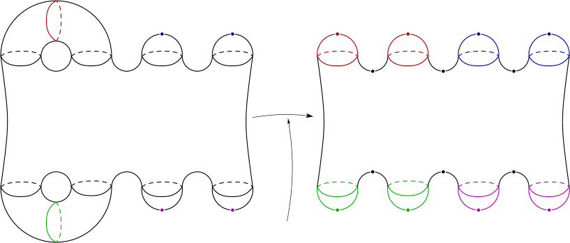
Figure 1. We remove tubular neighborhoods of the $\mu_{i}$, $i=1,\dots,g$, and then cap off the boundary components with disks. There, we define a Morse function $f$ whose gradient admits the singularities as indicated in the right of this Figure with the numbers indicating the indices of the singularities.

Proof of Theorem 1.1.

Given a Seifert manifold $Y=\mathbb{F}^{g}_{e}(r_{1},\dots,r_{k})$, pick a homology class $\mathfrak{c}$ which is given by

$$\mathfrak{c}=\sum_{i=1}^{g}\lambda_{i}[\beta_{i}]+\sum_{j=0}^{k}\alpha_{j}[\gamma_{j}]=\sum_{i=1}^{g}\lambda_{i}[\beta_{i}]+\alpha_{0}[\gamma_{0}]+\sum_{j=1}^{k}\alpha_{j}[\gamma_{j}],$$

where $\lambda_{i}$, $i=1,\dots,g$, and $\alpha_{j}$, $j=0,\dots,k$ are all elements in $\mathbb{Z}\backslash\{-1,0,1\}$. Let us call these classes maximal. We separated the summand $\alpha_{0}[\gamma_{0}]$ from the other $[\gamma_{j}]$’s, because this element just appears for $e\not=\pm 1$. We now fix a maximal class $\mathfrak{c}$. For every homology class $\mathfrak{h}\in H_{1}(Y;\mathbb{Z})$ we may apply the construction process described in §2 to get a nMS vector field in that homology class. Its number of periodic orbits shall be denoted by $n(Y,\mathfrak{h})$. Then it is easy to see that $n(Y,\mathfrak{c})\geq n(Y,\mathfrak{h})$ for all $\mathfrak{h}\in H_{1}(Y;\mathbb{Z})$. Furthermore, for every other maximal homology class $\mathfrak{d}$ we see that $n(Y,\mathfrak{d})=n(Y,\mathfrak{c})$. Recall from §2 that adjusting the homotopy class of a vector field (while fixing its homology class) creates $6$ additional periodic orbits. Hence, $n(Y)\leq n(Y,\mathfrak{c})+6$ which provides an upper bound for $n(Y)$. The crucial ingredient is to generate a Morse-Smale flow on the base $\Sigma$ with periodic orbits in the homology classes of $\pi(\beta_{i})$, $i=1,\dots,g$ and singularities at the points $\pi(\gamma_{j})$, $j=0,\dots,k$: Recall that a nMS vector field can be given by a round handle decomposition. Furthermore, observe that a Morse-Smale vector field without periodic orbits can be viewed as the gradient of a Morse function, which in turn defines a handle decomposition. Hence, to provide a Morse-Smale vector field on $\Sigma$ with the desired non-wandering set, we will cut the surface into two pieces, $\Sigma=F_{0}\cup_{\partial}F_{1}$, where $F_{0}$ is given by a round handle decomposition and $F_{1}$ by a handle decomposition (or, equivalently, by a Morse function). Hence, we will get Morse-Smale vector fields $X_{i}$, $i=0,1$, such that $X_{0}$ is non-singular and $X_{1}$ has singularities but no periodic orbits. In this way, we have precise control of the non-wandering set of $X_{0}\cup_{\partial}X_{1}$. To provide the upper bound, we have to move through a couple of different cases. We will discuss the first case thoroughly to point out that the proof technique works and then discuss the other cases in a brief way:
Case 1 – $g>0$, $e\not=\pm 1$, $n\geq 0$: The surface $\Sigma$ is of genus $g$ and, hence, can be written as a connected sum of $g$ tori $T^{2}_{1}\#T^{2}_{2}\#\dots\#T^{2}_{g}$. Furthermore, $\pi(\beta_{i})$, $i=1,\dots,g$, sits in the torus component $T^{2}_{i}$. Hence, after applying a suitable diffeomorphism $\phi\colon\thinspace\Sigma\longrightarrow\Sigma$, we may think of $\pi(\beta_{i})$ as a meridian $\mu_{i}$ of $T^{2}_{i}$. Removing tubular neighborhoods $\nu\mu_{i}$, $i=1,\dots,g$, we obtain a sphere with $2g$ holes, $S$ say. The holes of the surface should be grouped in pairs such that the pairs belong to the same meridian $\mu_{i}$. We cap off the boundary components with disks and obtain a sphere as indicated in Figure 1. We define a Morse function $f$ on this sphere with critical points of index $0$ or $2$ at the singularities $p_{i}$, $i=0,\dots,k$, and with singularities of index $0$ or $2$ at the centers of the capping disks. The function should be defined in such a way that the gradient is Morse-Smale. In other words, there should not be any separatrices connecting critical points of index $1$. To demonstrate that this can be realized, we provide a handle decomposition in Figure 2. This figure shows a handle decomposition of the sphere with $1$-handles which are not attached to each other.

2pt

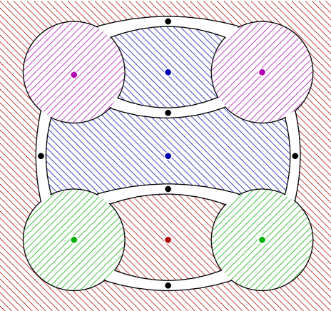
Figure 2. A handle decomposition of $\mathbb{S}^{2}$. The coloring coincides with the coloring given in Figure 1. The white strips are the $1$-handles in this handle decomposition. The associated Morse function has a Morse-Smale gradient. The points are the singularities of the gradient where one red point sits at infinity. The indices of the singularities are given in Figure 1.

Then we set $\Bigl{.}X_{1}\Bigr{|}_{S}=\Bigl{.}(\phi^{-1})_{*}(\nabla f)\Bigr{|}_{S}$. Observe that $\Sigma\backslash S$ is a union of cylinders, i.e. of $2$-dimensional round handles. On these round handles we define $X_{2}$ to equal the standard model of a Morse-Smale flow on a round handle: More precisely, every component of $\Sigma\backslash S$ is diffeomorphic to $\mathbb{S}^{1}\times[-1,1]$ with coordinates $t$ and $x$. On each of these components we require the vector field $X_{2}$ to equal $\partial_{t}-x\partial_{x}$ if $\mu_{i}$ is an attracting periodic orbit and $\partial_{t}+x\partial_{x}$ if it is a repelling periodic orbit. The vector field $X_{\Sigma}$, which is obtained by gluing together $X_{1}$ and $X_{2}$, is a Morse-Smale vector field with periodic orbits the $\mu_{i}$, $i=1,\dots,g$, with singularities the $\pi(\gamma_{j})$, $j=0,\dots,n$, which are either attracting or repelling, and with $2g+n-1$ singularities which are all saddles. To this vector field $X_{\Sigma}$ we apply the algorithm described in the previous section. We first lift this vector field to a vector field on the Seifert manifold. This lift admits $g$ invariant tori, $n+1$ singularities which are either attracting or repelling, and $2g+n-1$ saddle orbits. The destruction of the invariant tori (in the sense of Proposition 3.3) and the application of the 5th operation of Wada (cf. §2) leaves us with $n(Y,\mathfrak{c})=2g+3(n+1)+2g+n-1$ periodic orbits. Finally, we adjust the homotopy class (within its homology class) which creates $6$ additional periodic orbits. We get

$$n(Y)\leq n(Y,\mathfrak{c})+6=2g+3(n+1)+2g+n-1+6=4g+4n+8,$$

which ends the first case.
Case 2 – $g>0$, $e=\pm 1$, $n\geq 0$: This case differs from the first just by its Euler number. If the Euler number is $\pm 1$, then the regular fibers are nullhomologous. Hence, for every class $\mathfrak{c}$ the coefficient $\alpha_{0}$ will vanish. We proceed as before and generate $X_{\Sigma}$ with $g$ periodic orbits, $n$ singularities which are attractors/repellors and $2g+n-2$ saddles. Then we lift this vector field, destroy the invariant tori, perform the 5th operation of Wada and get

$$n(Y)\leq n(Y,\mathfrak{c})+6=2g+3n+2g+n-2+6=4g+4n+4,$$

which completes the second case.
Case 3 – $g=n=0$, $e\not=\pm 1$: The base space is a sphere and we need an arbitrary Morse-Smale vector field on the base, i.e. we put no requirements on the set of periodic orbits or the set of singularities. However, every gradient of a Morse function on the sphere has at least two singularities. So, we pick such a gradient and perform the algorithm presented in the previous section. The vector field lifts to a Morse-Smale field on the Seifert manifold with $2$ periodic orbits. We have to apply the 5th operation of Wada on one of these orbits and then we have to adjust the homotopy class (within its homology class) which generates additional $6$ periodic orbits. We obtain $n(Y)\leq 3+1+6=10$.
Case 4 – $g=n=0$, $e=\pm 1$: We pick the same vector field on the base as in the third case. The lift is Morse-Smale with two periodic orbits. We adjust the homotopy class which generates $6$ additional periodic orbits. We obtain $n(Y)\leq 2+6=8$.

∎

4. Extension to Graph Manifolds

Recall that a $3$-dimensional manifold $Y$ is called graph manifold if its prime decomposition consists of manifolds $Y_{1},\dots,Y_{n}$ such that in every $Y_{j}$, $j=1,\dots,n$, there exists a minimal collection of disjointly embedded tori such that the complement of these tori is a disjoint union of Seifert manifolds $Y_{n_{i}}^{g_{i};k_{i}}$, $i=1,\dots,l$. Here, $Y_{n_{i}}^{g_{i};k_{i}}$ denotes a Seifert manifold with genus-$g_{i}$ base with $k_{i}$ boundary components and $n_{i}$ exceptional orbits. Such a decomposition into Seifert manifolds is called a JSJ decomposition. We will first restrict to irreducible graph manifolds $Y$. To derive an upper bound we follow the natural approach: We will produce nMS vector fields on $Y$ by gluing together nMS vector fields from the Seifert pieces $Y_{n_{i}}^{g_{i};k_{i}}$ together. There are two constructions we have to provide: We have to generate a reference vector field to determine the homology classes of vector fields (cf. §2). And furthermore, we have to generate nMS vector fields on the pieces $Y_{n_{i}}^{g_{i};k_{i}}$ in such a way that these vector fields glue together to a vector field on $Y$ that is nMS.

4.1. The Reference Vector Field

Recall that for closed Seifert manifolds there exists a surgical presentation as introduced in §2. For a Seifert manifold with boundary we can also provide such a description in an analogous manner. Just note, that the base is a surface with boundary and that all $\mathbb{S}^{1}$-bundles over such are trivial. For every Seifert piece $Y_{n_{i}}^{g_{i};k_{i}}$ we pick such a presentation. The manifold $Y_{n_{i}}^{g_{i};k_{i}}$ admits a natural vector field $X_{\rm fiber}$ which is tangent to the fibers. The presentation of $Y_{n_{i}}^{g_{i};k_{i}}$ we have chosen induces a preferred collar neighborhood for all of its boundary components. Given such a boundary component, we have a preferred identification of a neighborhood with $[0,1]\times\mathbb{S}^{1}$. Denote by $\partial_{r}$ the vector field in the direction of the interval. So, in a collar neighborhood of the boundary we perturb $X_{\rm fiber}$ to $X_{0}=f\cdot X_{\rm fiber}+g\cdot\partial_{r}$, where $f$ is a non-negative function which is zero in a neighborhood of the boundary and increases to one as we move away from the boundary. And $g$ is a non-negative function which behaves in the opposite way as $f$, i.e. it is zero away from the boundary and it smoothly increases to one as we approach the boundary. We perform this construction with every Seifert piece and then glue the vector fields together to obtain one on the manifold $Y$. We will denote this vector field by $X_{0}$. This will serve us as our reference vector field.

4.2. The Construction Method

Constructing nMS vector fields on Seifert pieces with boundary in principle works the same way as done in the previous section. By a Mayer-Vietoris argument it is not hard to see that every homology class $\alpha$ can be written as

(4.1) $$\alpha=\sum_{a=1}^{g_{i}}\lambda_{a}\cdot[\beta_{a}]+\sum_{b=0}^{n_{i}}\alpha_{b}[\gamma_{b}]+\sum_{c=1}^{k_{i}-1}\tau_{c}[\delta_{c}],$$

where the $\beta_{a}$ are primitive elements in the homology of the surface, the $\gamma_{b}$, $b\not=0$, are the exceptional orbits, $\gamma_{0}$ is a regular fiber, and the $\delta_{c}$ are closed curves parallel to the boundary components of the surface. We proceed as before and create a Morse-Smale vector field $X_{\Sigma}$ on the base with the points $\pi(\gamma_{1}),\dots,\pi(\gamma_{n_{i}})$ as singularities and the curves $\beta_{1},\dots,\beta_{g_{i}}$ and $\delta_{1},\dots,\delta_{k_{i}-1}$ as periodic orbits. We lift this vector field with the procedure given in the previous sections (using $\left.X_{0}\right|_{Y_{n_{i}}^{g_{i};k_{i}}}$ instead of $X_{\rm fiber}$) and then destroy the invariant tori (in the sense of Proposition 3.3) over both the $\beta$-curves and the $\delta$-curves. The destruction is done such that we create periodic orbits whose homology classes represent $\lambda_{a}\cdot[\beta_{a}]$ and $\tau_{c}\cdot[\delta_{c}]$. Then the 5th operation of Wada will allow us to replace $\gamma_{b}$, $b=0,\dots,n_{i}$, by a periodic orbit which represents the class $\alpha_{b}\cdot[\gamma_{b}]$, $b=0,\dots,n_{i}$. Finally, we make the vector field transverse to the boundary components like done for the reference vector field. Performing this construction for every piece $Y_{n_{i}}^{g_{i};k_{i}}$, these vector fields can be glued together to provide a nMS vector field on $Y$ whose set of periodic orbits contains a link $L$ consisting of attractive or repulsive orbits such that $[L]=\mathfrak{c}$ for every given $\mathfrak{c}$.

4.3. The Proofs of the Main Results

Before delving into the proof we would like to state the following result of Yano which will be used in the proof of Theorem 1.2.

Proposition 4.1 (Theorem 1 of [10]).

Let $Y$ be a graph manifold prime to $\mathbb{S}^{2}\times\mathbb{S}^{1}$ and $\rho\colon\thinspace Y\longrightarrow\mathcal{C}_{Y}$ the natural map into the Jaco-Shalen-Johansson complex of $Y$. Then the homotopy class of a vector field $X$ admits a (non-singular) Morse-Smale representative if and only if $\rho_{*}(e(X))$ vanishes in $H_{1}(\mathcal{C}_{Y};\mathbb{Z})$, where $e(X)$ is the Poincaré dual of the Euler class of the field of $2$-planes orthonormal to $X$.

Furthermore, note that there are also homotopical invariants for vector fields on manifolds with boundary (cf. for instance [10, p. 439]). In §2 we briefly introduced the geometric interpretation of homology classes of vector fields. This is based on the Pontryagin construction which is described in [5, §7]. The Pontryagin construction as described in [5, §7] can be adapted to work for the case of manifolds with boundary. Then for two vector fields $X_{1}$, $X_{2}$ on a manifold $Y$ with non-trivial boundary, the homology class of $C_{-}(X_{1},X_{2})$ measures the homotopical distance away from the $3$-cells of $Y$ as in the closed case. However, in the case of non-empty boundary, the vector fields are understood to be in a pre-chosen homotopy class along the boundary of $Y$ (cf. [10, p. 439] and [10, Lemma 1.5]).

Because the homotopical classification of vector fields on manifolds with boundary works the same way as in the closed case, we can apply our algorithm to the Seifert pieces $Y_{j}$ of a JSJ decomposition of a graph manifold to obtain upper bounds for the $n(Y_{j})$.

Proof of Theorem 1.2.

The homology classes in the kernel of $\rho_{*}$ are contained in the image of the map

(4.2) $$\bigoplus_{i=1}^{l}H_{1}(Y_{n_{i}}^{g_{i};k_{i}};\mathbb{Z})\longrightarrow H_{1}(Y;\mathbb{Z})$$

given by the obvious Mayer-Vietoris sequence (cf. [10, p. 444]). Denote by $\mathfrak{e}$ the homology class of the reference vector field $X_{0}$ (cf. §4.1). By the considerations from above we can glue together nMS vector fields on the pieces to obtain a nMS vector field on $Y$. If we do this as before, we can define a nMS vector field $X$ on $Y$ such that $C_{-}(X,X_{0})$ is empty and, hence, $\mathfrak{e}$ can be written as a sum $\mathfrak{e}_{i}\in H_{1}(Y_{n_{i}}^{g_{i};k_{i}};\mathbb{Z})$, $i=1,\dots,l$ (cf. Proposition 4.1). So, suppose we are given a class $\mathfrak{c}\in H_{1}(Y;\mathbb{Z})$ which can be written as a sum of classes $\mathfrak{c}_{i}\in H_{1}(Y_{n_{i}}^{g_{i};k_{i}};\mathbb{Z})$, $i=1,\dots,l$. Then by the previous discussion, we see that on every piece $Y_{n_{i}}^{g_{i};k_{i}}$ there exists a nMS vector field $X_{i}$ whose set of periodic orbits contains a link $L_{i}$ consisting of attracting and repelling periodic orbits such that $[L_{i}]=\mathfrak{c}_{i}-\mathfrak{e}_{i}$. We glue the $X_{i}$ together to obtain a nMS vector field $X$ on $Y$. Hence, the set of periodic orbits of $X$ contains the link $L=L_{1}\cup\dots\cup L_{l}$. Then $C_{-}(X,X_{0})$ is empty and, so, they lie in the same homology class. We generate a new nMS vector field by reversing the orientation of the periodic orbits contained in $L$. Denote the new vector field by $X^{\prime}$. Then, we have

$$[X^{\prime}]=[C_{-}(X^{\prime},X_{0})]+[X_{0}]=[L]+\mathfrak{e}=\mathfrak{c}-\mathfrak{e}+\mathfrak{e}=\mathfrak{c}.$$

The maximal number of periodic orbits will be given when choosing a class $\mathfrak{c}-\mathfrak{e}$ whose presentation in the form of Equation (4.1) has the property that $\lambda_{a}\not\in\{-1,0,1\}$ for all $a=1,\dots,g_{i}$, $\gamma_{b}\not\in\{-1,0,1\}$ for $b=0,\dots,n_{i}$, and $\delta_{c}\not\in\{-1,0,1\}$ for $c=1,\dots,k_{i}-1$. So, a maximal class in the graph manifold is a sum of maximal classes of the Seifert pieces. Hence, our previous considerations, i.e. especially the proof Theorem 1.1, provides us with the upper bound

$$n(Y_{n_{i}}^{g_{i};k_{i}})\leq 4g+4n+8+2\delta_{g_{i},0}\delta_{n_{i},0}+2(k_{i}-1)$$

for every $i=1,\dots,l$. Observe that in this bound we already included the changes to adapt the homotopy classes within a fixed homology class. Hence, for $l>1$ we have

$$n(Y)\leq 6+\sum_{i=1}^{l}n(Y_{n_{i}}^{g_{i};k_{i}})-6,$$

which is equivalent to $n(Y)\leq 6+2\cdot\sum_{i=1}^{l}\bigl{(}2g_{i}+2n_{i}+\delta_{g_{i},0}\delta_{n_{i},0}+k_{i}\bigr{)}.$ ∎

Proof of Corollary 1.3.

This statement immediately follows from our discussion and the observation that it is possible to define connected sums of nMS vector fields on manifolds and that their homotopical invariants behave additive under connected sums. This was observed by Yano in [10, §2] (especially [10, Proposition 2.8]). ∎

References

- [1] D. Asimov, Homotopy of non-singular vector fields to structurally stable ones, Ann. Math. (1)102 (1975), 55–65.
- [2] E. Dufraine, Classes d’homotopie de champs de vecteurs Morse-Smale sans singularité sur les fibrés de Seifert, Enseign. Math. (2)51 (2005), 3–30.
- [3] E. Dufraine, About homotopy classes of non-singular vector fields on the three-sphere, Qual. Theory Dyn. Syst. 3 (2002), 361–376
- [4] H. Geiges, An Introduction to Contact Topology, Cambridge Studies in Advanced Mathematics 109, Cambridge University Press, 2008.
- [5] J. Milnor Topology from the Differentiable Viewpoint, The University Press of Virginia, 1965.
- [6] W.D. Neumann and L. Rudolph, Difference index of vector fields and the enhanced Milnor number, Topology 29 (1990), 83–100.
- [7] C. Robinson, Dynamical Systems – Stability, Symbolic Dynamics and Chaos, Studies in Advanced Mathematics, (2nd edition), CRC Press, (1999).
- [8] M. Wada, Closed orbits of non-singular Morse-Smale flows on , J. Math. Soc. Japan 41(3) (1989), 405–413.
- [9] F.W. Wilson, Some examples of nonsingular Morse-Smale vector fields on , Ann. Inst. Fourier 27 (1977), 145–159.
- [10] K. Yano, The homotopy class of non-singular Morse-Smale vector fields on -manifolds, Invent. Math. 80 (1985), 435–451.