Nash Codes for Noisy Channels

Abstract

This paper studies the stability of communication protocols that deal with transmission errors. We consider a coordination game between an informed sender and an uninformed decision maker, the receiver, who communicate over a noisy channel. The sender’s strategy, called a code, maps states of nature to signals. The receiver’s best response is to decode the received channel output as the state with highest expected receiver payoff. Given this decoding, an equilibrium or “Nash code” results if the sender encodes every state as prescribed. We show two theorems that give sufficient conditions for Nash codes. First, a receiver-optimal code defines a Nash code. A second, more surprising observation holds for communication over a binary channel which is used independently a number of times, a basic model of information transmission: Under a minimal “monotonicity” requirement for breaking ties when decoding, which holds generically, every code is a Nash code.

Keywords: sender-receiver game, communication, noisy channel.

1 Introduction

Information transmission is central to the interaction of economic agents and to the operation of organizations. This paper presents a game-theoretic analysis of communication with errors over a “noisy channel”. The noisy channel is a basic model of information theory, pioneered by Shannon (1948), and fundamental for the design of reliable data transmission. In this model, an informed sender sends a message, which is distorted by the channel, to an uninformed receiver. Sender and receiver have the common interest that the receiver understands the sender as reliably as possible.

A communication protocol defines a code, that is, a set of channel inputs that represent the possible messages for the sender, and a way for the receiver to decode the channel output. One can view the designer of the protocol as a “social planner” who tries to solve an optimization problem, for example to achieve high reliability and a good rate of information transmission. This assumes that sender and receiver adhere to the protocol. In this paper, we study this model as a game between sender and receiver as two players. A strategy of the sender is a code, and a strategy of the receiver is a way to decode the channel output. Rather than requiring that sender and receiver adhere to their respective strategies, we assume that they can choose their strategies freely. A Nash equilibrium is a pair of strategies for sender and receiver that are mutual best responses. This is the central stability concept of game theory.

The best response of the receiver is known in the communications literature as MAP (maximum a posteriori) decoding. In contrast, allowing the sender to deviate from the code (while the receiver strategy is fixed) is specific to the game-theoretic approach. If the sender is not in equilibrium, she has an incentive to change her strategy to encode some message with a different codeword. If this happens, the protocol will lose its function as a de-facto standard of communication. The appeal of a Nash equilibrium is that it is self-enforcing.

Sender-receiver games have attracted significant interest in economics (Spence, 1973; Crawford and Sobel, 1982). The game-theoretic view is also applied in models of language evolution (Nowak and Krakauer, 1999; Argiento et al., 2009). These assume, as in our case, that the interests of sender and receiver are fully aligned, and use Nash equilibrium as the natural stability criterion. We survey this related literature in more detail below. In the analysis and design of communication networks, a growing body of research deals with game-theoretic approaches that assume selfish agents (Srivastava et al., 2005; MacKenzie and DaSilva, 2006; Anshelevich et al., 2008), again with Nash equilibrium as the central solution concept.

The model

We consider the classic model of the discrete noisy channel. The channel has a finite set of input and output symbols and known transition probabilities that represent the possible communication successes and errors. The channel may also be used repeatedly, with independent errors. In the important case of the binary channel that has only two symbols, the codewords are then fixed-length sequences of bits.

In our sender-receiver game, nature chooses one of finitely many states at random according to a prior probability. The sender is informed of the state and transmits a signal via the discrete noisy channel to the uninformed receiver who makes a decision. The sender’s strategy or code assigns to each state of nature a specific signal or “codeword” that is the input to the channel. The receiver’s strategy decodes the distorted signal that is the channel output as one of the possible states. Both players receive a (possibly different) positive payoff only if the state is decoded correctly, otherwise payoff zero.

In equilibrium, the receiver decodes the channel output as the state with highest expected payoff. When all states get equal receiver payoff, the receiver condition is the well-known MAP decoding rule (MacKay, 2003, p. 305). The equilibrium condition for the sender means that she chooses for each state the prescribed codeword as her best response, that is, no other channel input has a higher probability of being decoded correctly with the given receiver strategy.

A Nash code is a code together with a best-response decoding function that defines a Nash equilibrium. So we assume the straightforward equilibrium condition for the receiver and require that the code fulfills the more involved sender condition. (Of course, both conditions are necessary for equilibrium.)

Our results

We present two main results about Nash codes, along with other observations that we describe in the outline of our paper at the end of this introduction. Our first main result concerns discrete channels with arbitrary finite sets of input and output symbols. We show that already for three symbols, not every code defines a Nash equilibrium. However, a Nash code results if the expected payoff to the receiver cannot be increased by replacing a single codeword with another one (Theorem 4.4). So these receiver-optimal codes are Nash codes. This is closely related to potential games (Proposition 4.5), which may provide the starting point for studying dynamics of codes until they become Nash codes, as a topic for further research.

In short, without any constraints on the channel, and for any best-response decoding, receiver-optimal codes are Nash codes. For equal receiver utilities for each state, these are the codes with maximum expected reliability, which therefore implies Nash equilibrium. The method to show this result is not deep; its purpose is to analyze our model. The key assumption is that an improvement in decoding probability benefits both sender and receiver. However, a sender-optimal code is not necessarily a Nash code if sender and receiver give different utilities to a correct decoding of the state of nature. This happens if the sender can use an unused message to transmit the information about the state more reliably. If all channel symbols are used, then under reasonable assumptions the code is Nash (see Proposition 3.1).

Our second main result is more surprising and technically challenging. It applies to the binary channel where codewords are strings of bits with independent positive error probabilities for each bit. Then every code is a Nash code (Theorem 6.5), irrespective of its quality. The only requirement for the decoding is that the receiver breaks ties between states monotonically, that is, in a consistent manner; this holds for natural tie-breaking rules, and ties do not even occur if states of nature have different generic prior probabilities or utilities. That is, for the binary channel, as long as the receiver decodes optimally and breaks ties consistently, the equilibrium condition holds automatically on the sender’s side.

Binary codes are fundamental to the practice and theory of information theory. Our result that they are Nash codes shows that they are incentive compatible. Hence, this condition is orthogonal to engineering issues such as high reliability and rate of information transmission.

Related literature

Information transmission is often modeled in the economic literature as a sender-receiver game between an informed expert and an uninformed decision maker. Standard signaling models (pioneered by Spence, 1973) often assume that signals have costs associated with the information of the sender. In their seminal work on strategic information transmission, Crawford and Sobel (1982) consider costless signals and communication without transmission errors, but where the incentives of sender and receiver differ. They assume that a fixed interval represents the set of possible states, messages, and receiver’s actions. Payoffs depend continuously on the difference between state and action, and differ for sender and receiver. In equilibrium, the interval is partitioned into finitely many intervals, and the sender sends as her message only the partition class that contains the state. Thus, the sender only reveals partial information about the state. Along with many other models (see the surveys by Kreps and Sobel, 1994, and Sobel, 2013), this shows that information is not transmitted faithfully for strategic reasons because of some conflict of interest.

Even in rather simple sender-receiver games, players can get higher equilibrium payoffs when communicating over a channel with noise than with perfect communication (Myerson, 1994, Section 4). Blume, Board, and Kawamura (2007) extend the model by Crawford and Sobel (1982) by assuming communication errors. The noise allows for equilibria that improve welfare compared to the Crawford–Sobel model. The construction partly depends on the specific form of the errors so that erroneous transmissions can be identified; this does not apply in our discrete model. In addition, in our model players only get positive payoff when the receiver decodes the state correctly, unlike in the continuous models by Crawford and Sobel (1982) and Blume et al. (2007). On the other hand, compared to perfect communication, noise may prevent players from achieving common knowledge about the state of nature (Koessler, 2001).

Game-theoretic models of communication have been used in the study of language (see De Jaegher and van Rooij, 2013, for a recent survey). Lewis (1969) describes language as a “convention” with mappings between states and signals, and argues that these should be bijections. Nowak and Krakauer (1999) use evolutionary game theory to show how languages may evolve from “noisy” mappings; Wärneryd (1993) shows that only bijections are evolutionary stable. However, even ambiguous sender mappings (where one signal is used for more than one state) together with a mixed receiver population may be “neutrally stable” (Pawlowitsch, 2008); the randomized receiver strategy can be seen as noise. Argiento et al. (2009) consider the learning process of a language in a sender-receiver game. This is extended to the noisy channel by Touri and Lambort (2013).

Blume and Board (2013) use the noisy channel to model vagueness in communication. Lipman (2009) discusses how vagueness can arise even for coinciding interests of sender and receiver. Ambiguous signals arise when the set of messages is smaller than the set of states, which may reflect communication costs for the sender (see Jäger, Koch-Metzger, and Riedel, 2011, and the discussion in Sobel 2012). For the sender-receiver game with a noisy binary channel, Hernández, Urbano, and Vila (2012) describe the equilibria for a specific code that can serve as a “universal grammar”; the explicit receiver strategy allows to characterize the equilibrium payoff.

Noise in communication is relevant to models of persuasion, where the sender wants to induce the receiver to take an action. Glazer and Rubinstein (2004; 2006) study binary receiver actions; the sender may reveal limited information about the state of nature as “evidence”. The optimal way to do so is a receiver-optimal mechanism. In a more general setting, Kamenica and Gentzkow (2011) allow the sender to commit to a strategy that selects a message for each state, assuming the receiver’s best response using Bayesian updating; the sender may generate noise by selecting the message at random. Subject to a certain Bayesian consistency requirement, the sender can commit to her best possible strategy.

Equilibrium models of information transmission give several insights. First, communication may fail: Every sender-receiver game has a “babbling equilibrium” where the sender’s action is independent of the state and the receiver’s action is independent of the channel output, with no information transmitted. Second, equilibria are typically not unique (for example, mapping states to signals is often arbitrary). Third, conflict of interest, or cost and complexity of communication (Sobel, 2012), prevent perfect communication.

Our approach takes a basic view that communication can be impeded by noise when interests of sender and receiver are aligned, and analyzes this issue game-theoretically. Our results show that the Nash equilibrium condition is weaker than or, for the binary channel, orthogonal to the quality of information transmission.

Outline of the paper

Section 2 describes our model and characterizes the Nash equilibrium condition. For channels with any number of symbols, Section 3 gives examples that some codes may not be Nash codes. Section 4 shows that receiver-optimal codes are Nash, and discusses the relation to potential functions. In Section 5, we consider binary codes, where we first demonstrate that tie-breaking needs to be “monotonic” when ties occur in order for Nash equilibrium to hold for every code. In Section 6 we show the main Theorem 6.5 that every monotonically decoded binary code is Nash. This holds in fact not just for binary codes but for any “input symmetric” channels with any number of symbols where the probability of receiving a symbol incorrectly does not depend on the channel input. The proof also shows that the property of a channel that every code is Nash, which we call “Nash-stability”, extends to any product of channels (see Section 7) with independent errors. The product channel assumes independent error probabilities, but the codewords are still arbitrary combinations of inputs for such products. (If the error probabilities are not independent, then the channel has to be considered with $n$-tuples as input and output symbols where in general only Theorem 4.4 about receiver-optimal codes applies.) A natural monotonic decoding rule is to break ties according to a fixed order among the states, as when they have generic priors. In Section 8 it is shown that this is in fact the only general deterministic monotonic tie-breaking rule.

2 Nash codes

We consider a game of two players, a sender (she) and a receiver (he). First, nature chooses a state $i$ from a set $\Omega=\{0,1,\ldots,M-1\}$ with positive prior probability $q_{i}$. Then the sender is fully informed about $i$, and sends a message to the receiver via a noisy channel. After receiving the message as output by the channel, the receiver takes an action that affects the payoff of both players.

The channel has finite sets (or “alphabets”) $X$ and $Y$ of input and output symbols, with noise given by transition probabilities $p(y|x)$ for each $x$ in $X$ and $y$ in $Y$. The channel is used $n$ times independently without feedback. When an input $x=(x_{1},\ldots,x_{n})$ is transmitted through the channel, it is altered to an output $y=(y_{1},\ldots,y_{n})$ according to the probability $p(y|x)$ given by

$$p(y|x)=\prod_{j=1}^{n}p(y_{j}|x_{j}).$$ (1)

This is the standard model of a memoryless noisy channel as considered in information theory (see Cover and Thomas, 1991; Gallager, 1968; MacKay, 2003).

The sender’s strategy is to encode state $i$ by means of a coding function or code $c:\Omega\to X^{n}$, which we write as $c(i)=x^{i}$. We call $x^{i}$ the codeword or message for state $i$ in $\Omega$, which the sender transmits as input to the channel. The code $c$ is completely specified by the list of $M$ codewords $x^{0},x^{1},\ldots,x^{M-1}$, which is called the codebook.

The receiver’s strategy is to decode the channel output $y$, given by a probabilistic decoding function

$$d:Y^{n}\times\Omega\to{\mathbb{R}},$$ (2)

where $d(y,i)$ is the probability that $y$ is decoded as $i$.

If the receiver decodes the channel output as the state $i$ chosen by nature, then sender and receiver get positive payoff $U_{i}$ and $V_{i}$, respectively, otherwise both get payoff zero. The incentives of sender and receiver are fully aligned in the sense that they always prefer that the state is communicated successfully. However, the importance of that success may be different for sender and receiver depending on the state. The channel transition probabilities, the transmission length $n$, and the prior probabilities $q_{i}$ and utilities $U_{i}$ and $V_{i}$ for $i$ in $\Omega$ are commonly known to the players.

Definition 2.1.

Consider an encoding function $c:\Omega\to X^{n}$ and a probabilistic decoding function $d$ in $(\ref{dec})$. If the pair $(c,d)$ defines a Nash equilibrium, then $c$ is called a Nash code. The expected payoffs to sender and receiver are denoted by $U(c,d)$ and $V(c,d)$, respectively.

In order to obtain a Nash equilibrium $(c,d)$, receiver and sender have to play mutually best responses. The equilibrium property, and whether $c$ is called a Nash code as part of such an equilibrium, may depend on the particular best response $d$ of the receiver.

A code $c$ defines the sender’s strategy. A best response of the receiver is the following. Given that he receives channel output $y$ in $Y^{n}$, the probability that codeword $x^{i}$ has been sent is, by Bayes’s law, $q_{i}\,p(y|x^{i})/\hbox{prob}(y)$, where $\hbox{prob}(y)$ is the overall probability that $y$ has been received. The factor $1/\hbox{prob}(y)$ can be disregarded in the maximization of the receiver’s expected payoff. Hence, a best response of the receiver is to choose with positive probability $d(y,i)$ only states $i$ so that $q_{i}V_{i}\,p(y|x^{i})$ is maximal, that is, so that $y$ belongs to the set $Y_{i}$ defined by

$$Y_{i}=\{y\in Y^{n}\mid q_{i}V_{i}\,p(y|x^{i})\geq q_{k}V_{k}\,p(y|x^{k})~{}~{}\forall k\in\Omega\}.$$ (3)

Hence, the best response condition for the receiver states that for any $y\in Y^{n}$ and $i\in\Omega$

$$d(y,i)>0\quad\Rightarrow\quad y\in Y_{i}\,.$$ (4)

If $V_{i}=1$ for all $i\in\Omega$, then this decoding rule is known as MAP or maximum a posteriori decoding (MacKay, 2003, p. 305). If the receiver has different positive utilities $V_{i}$ for different states $i$, then the receiver’s best response maximizes $q_{i}V_{i}\,p(y|x^{i})$. We call the product $q_{i}V_{i}$ the weight for state $i$. One could assume $V_{i}=1$ for all $i$ and only vary $q_{i}$ in place of the weight, but then it seems artificial to allow separate utilities $U_{i}$ for the sender, because we want to study the Nash property with respect to the optimality of codes for receiver and sender. For that reason we keep three parameters $q_{i}$, $U_{i}$ and $V_{i}$ for each state $i$.

We say that for a given channel output $y$, there is a tie between two states $i$ and $k$ (or the states are tied ) if $y\in Y_{i}\cap Y_{k}$. If there are never any ties, then the sets $Y_{i}$ for $i\in\Omega$ are pairwise disjoint, and the best-response decoding function is deterministic and unique according to (4). If there are ties, then a natural way to break them is to choose any of the tied states with equal probability. For that reason we consider probabilistic decoding functions. On the sender’s side, we only consider deterministic encoding strategies.

We sometimes refer to the sets $Y_{i}$ for $i\in\Omega$ as a “partition” of $Y^{n}$, which constrains the receiver’s best-response decoding as in (4), even though some of these sets may be empty, and they may not always be disjoint if there are ties. In any case, $Y^{n}=\bigcup_{i\in\Omega}Y_{i}$.

Suppose that the receiver decodes the channel output with $d$ according to (3) and (4) for the given code $c$ with $c(i)=x^{i}$. Then $(c,d)$ is a Nash equilibrium if and only if, for any state $i$, it is optimal for the sender to transmit $x^{i}$ and not any other $\hat{x}$ in $X^{n}$ as a message. When sending $\hat{x}$, the expected payoff to the sender in state $i$ is

$$U_{i}\sum_{y\in Y^{n}}p(y|\hat{x})\,d(y,i).$$ (5)

When maximizing (5) as a function of $\hat{x}$, the utility $U_{i}$ to the sender does not matter as long as it is positive; given that the state is $i$, the sender only cares about the expected probability that the channel output $y$ is decoded as $i$. We summarize these observations as follows.

Proposition 2.2.

The code $c$ with decoding function $d$ is a Nash code if and only if the receiver decodes channel outputs according to $(\ref{Yi})$ and $(\ref{arbtie})$, and if and only if in every state $i$ the sender transmits codeword $c(i)=x^{i}$ which fulfills for any other possible channel input $\hat{x}$ in $X^{n}$

$$\sum_{y\in Y^{n}}p(y|x^{i})\,d(y,i)\geq\sum_{y\in Y^{n}}p(y|\hat{x})\,d(y,i)\,.$$ (6)

3 Examples of codes that are not Nash

This section presents introductory examples of channels that are used once ($n=1$) and that illustrate that the Nash equilibrium condition does not hold automatically. At the end of this section, we show in Proposition 3.1 that, under certain assumptions, the Nash property holds when all channel symbols are used for transmission.

For our first example, consider a channel with three symbols, $X=Y=\{0,1,2\}$, which is used only once ($n=1$), with the following transition probabilities:

$$y$$

0 1 2

0 0.7 0.15 0.15

  1 0.25 0.5 0.25

2 0.2 0.2 0.6

(7)

Suppose that there are two states ($m=2$) and that nature chooses the two states from $\Omega=\{0,1\}$ with uniform priors $q_{0}=q_{1}=1/2$. The sender’s utilities are $U_{0}=2$ when the state is $0$ and $U_{1}=8$ when the state is 1, and the receiver’s utilities are $V_{0}=6$, $V_{1}=4$.

Consider the codebook $c$ with $c(0)=x^{0}=0$ and $c(1)=x^{1}=1$, so the sender codifies the two states of nature as the two symbols $0$ and $1$, respectively. Given the parameters of this game and the sender’s strategy $c$, the receiver’s strategy assigns to each output symbol in $\{0,1,2\}$ one state. The following table (8) gives the expected payoff $q_{i}V_{i}\,p(y|x^{i})$ for the receiver when the state is $i$ and the output symbol is $y$.

$$y$$

0 1 2

0 2.1 0.45 0.45

   1 0.5 1 0.5

(8)

This shows how to find the receiver’s best response and the sets $Y_{i}$ in (3). For each channel output $y$, the receiver chooses the state $i$ with highest expected payoff. Hence, he decodes the channel output $0$ as state $0$ because $q_{0}V_{0}\,p(0|x^{0})=2.1>0.5=q_{1}V_{1}\,p(0|x^{1})$. In the same way, he decodes both channel outputs $1$ and $2$ as state $1$. Here there are no ties, so the two sets $Y_{0}$ and $Y_{1}$ are disjoint, and the receiver’s best response is unique and deterministic. That is, the receiver’s best response $d$ is given by $d(y,i)=1$ if $y\in Y_{i}$, where $Y_{0}=\{0\}$ and $Y_{1}=\{1,2\}$, and by $d(y,i)=0$ otherwise.

A shorter form of obtaining (8) from the channel transition probabilities in (7) is shown in (9), which is (7) with each row prefixed by the weight $q_{i}V_{i}$ when the channel input for that row is used as codeword $x^{i}$. Multiplying the channel probabilities with these weights gives (8), and a box surrounds $p(y|x^{i})$ if output $y$ is decoded as state $i$. These boxes therefore also show the sets $Y_{i}$ if there are no ties, as in the present case; in the case of ties, and deterministic decoding, they show the state that is actually decoded by the receiver.

$$y$$

0 1 2

3 0 0.7 0.15 0.15

2   1 0.25 0.5 0.25

2 0.2 0.2 0.6

(9)

With the help of Proposition 2.2, it is easy to see from (9) that this code $c$ is not a Nash code. For $i=0$ and $x^{0}=0$, we have $\sum_{y\in Y}p(y|0)d(y,0)=0.7$, which is the maximum of the column entries $p(y|x)$ for $y=0$ in (9), so here the sender cannot improve her payoff by transmitting any $\hat{x}$ instead of $x^{i}$. However, for $i=1$ we have $\sum_{y\in Y}p(y|1)d(y,1)=0.5+0.25=0.75<0.8=0.2+0.6=\sum_{y\in Y}p(y|2)d(y,2)$, so (6) does not hold when $x^{i}=1$ and $\hat{x}=2$ and the sender can improve her payoff by sending $\hat{x}$ instead of $x^{i}$.

Is there a Nash code for the channel in (7) when $\Omega=\{0,1\}$ and for the described priors and utilities? First, a simple and trivial Nash code is to map both states to the same, arbitrary channel input, $x^{0}=x^{1}$. Then every channel output results from the same row (for that input) in (7) and, because $q_{0}V_{0}>q_{1}V_{1}$, will be decoded as state 0. The sender cannot improve her payoff because the receiver in effect ignores the uninformative channel output. This is also called a “babbling” or “pooling” equilibrium, which is a Nash equilibrium for any channel.

When the codewords are distinct ($x^{0}\neq x^{1}$), there are six possible ways to choose them from the three channel inputs. Table 1 lists these codebooks $x^{0},x^{1}$, shown in the first column. For each code, the receiver’s best response is unique. The best-response partition $Y_{0},Y_{1}$ is shown in the second column. Using this partition, the third column gives the probabilities $p(y\in Y_{i}\mid x^{i})=\sum_{y\in Y_{i}}p(y|x^{i})$ that the codeword $x^{i}$ is decoded correctly. The overall expected payoffs to sender and receiver are shown as $U$ and $V$, with a box indicating the respective maximum.

Table 1: Possible codebooks $x^{0},x^{1}$ with $x^{0}\neq x^{1}$ for the channel (7) and expected payoffs $U$ and $V$ to sender and receiver.

$$\begin{array}[]{|c|cc|cc|c|c|}\hline\cr~{}~{}x^{0},x^{1}{}{}&~{}~{}Y_{0}{}{}&~{}~{}Y_{1}{}{}&p(y\in Y_{0}\mid x^{0})&p(y\in Y_{1}\mid x^{1})&U&V\\ \hline\cr 0,1&\{0\}&\{1,2\}&0.70&0.75&~{}\framebox{3.70}{}&~{}~{}3.60{}{}\\ 0,2&\{0,1\}&\{2\}&0.85&0.60&~{}~{}3.25{}{}&3.75\\ 1,0&\{1,2\}&\{0\}&0.75&0.70&3.55&3.65\\ 1,2&\{0,1\}&\{2\}&0.75&0.60&3.15&3.45\\ 2,0&\{1,2\}&\{0\}&0.80&0.70&3.60&~{}\framebox{3.80}{}\\ 2,1&\{0,2\}&\{1\}&0.80&0.50&2.80&3.40\\ \hline\cr\end{array}$$

Similar to using (9) for the codebook $0,1$, it can be verified that the codebook $2,1$ is not a Nash code. In addition, Table 1 shows directly that the codebook $1,0$ is not a Nash code: It has the same best response of the receiver (given by $Y_{0}=\{1,2\}$ and $Y_{1}=\{0\}$) as the codebook $2,0$, but a lower payoff to the sender (3.55 instead of 3.6), who can therefore improve her payoff by changing $x^{0}=1$ to $\hat{x}=2$ (note that the receiver’s reaction stays fixed). Similarly, codebook $1,2$ has the same best response as $0,2$, but a lower payoff to the sender (3.15 instead of 3.25).

Only the codebooks $2,0$ and $0,2$ in Table 1 are Nash codes. Apart from a direct verification, this follows from Theorems 4.2 and 4.4, respectively, which we will discuss in the next section.

The fact that a code is not Nash seems to be due to the fact that not all symbols of the channels are used for transmission. With some qualifications, this is indeed the case, as we discuss in the remainder of this section.

Consider the channel in (7) and suppose that there are three states, $\Omega=\{0,1,2\}$. However, even when each state is assigned to a different input symbol, one can replicate the counterexample in (9) when the additional state $2$ has a weight $q_{2}V_{2}$ that is too low. For example, if priors are uniform as before ($q_{i}=1/3$) and $V_{0}=6$, $V_{1}=4$, and $V_{2}=1$, then the channel outputs would be decoded as before when state 2 is absent, with the same lack of the Nash property.

Hence, one should require that all output symbols are decoded differently. However, the following example shows that this may still fail to give a Nash code:

$$y$$

0 1 2

0.35 0 0.4 0.3 0.3

0.35   1 0.3 0.4 0.3

0.35 2 0.05 0.45 0.5

(10)

Suppose states 0, 1, 2 are encoded as 0, 1, 2 and have the indicated weights 0.35, 0.35, 0.3, respectively. Here, the row for channel input 1 has slightly higher weight than for input 2, so because $0.35\times 0.4>0.3\times 0.45$ the decoding function is just the identity. However, for state 1 the sender can improve the probability of correct decoding by deviating from $x^{1}=1$ to $\hat{x}=2$ because $0.4<0.45$.

In (10), for any input $x$ the corresponding output $y=x$ has the highest probability of arriving, but this is not relevant for decoding. With uniform priors and utilities, a reasonable condition for the channel is “identity decoding”, that is, for any received output $y$, the maximum likelihood input is $x=y$. That is, suppose that

$$X=Y,\qquad p(y|y)>p(y|x)\quad\hbox{for all }y\in Y,~{}x\in X,~{}x\neq y$$ (11)

which says that each output symbol $y$ is more likely to have been received correctly than in error. This property is violated in (10), but if it holds then the following proposition applies.

Proposition 3.1.

Consider a channel with input and output alphabets $X$ and $Y$ so that $(\ref{diag})$ holds. Let $c$ be a code so that each channel output is decoded as coming from a different channel input $x^{i}$ with a deterministic best-response decoding function $d$. Then $(c,d)$ is a Nash equilibrium and $c$ is a Nash code. Every output $y$ is decoded as a state $i$ so that $x^{i}=y$ and so that $q_{i}V_{i}$ is maximal.

Proof. By assumption, $X=Y$ and the map $\phi:Y\to X$ defined by $\phi(y)=x^{i}$ if $d(y,i)=1$ is injective and hence a bijection. Suppose $\phi$ is not the identity map, so it has a cycle of length $l>1$, which by permuting $\Omega$ we assume as coming form the first $l$ states $x^{0},x^{1},\ldots,x^{l-1}$, that is, $\phi(x^{j})=x^{j+1\hbox{mod}l}$ for $0\leq j<l$. So channel output $x^{0}$ is decoded as state 1 because $\phi(x^{0})=x^{1}$, output $x^{1}$ is decoded as state 2, and so on. Because $d$ is a best-response decoding function, $q_{0}V_{0}\,p(x^{0}|x^{0})\leq q_{1}V_{1}\,p(x^{0}|x^{1})$ and therefore

$$q_{0}V_{0}\leq q_{1}V_{1}\frac{p(x^{0}|x^{1})}{p(x^{0}|x^{0})}<q_{1}V_{1}$$

by (11). In the same manner, $q_{1}V_{1}<q_{2}V_{2}<\cdots<q_{l-1}V_{l-1}<q_{0}V_{0}$, a contradiction.

So $\phi$ is identity map. Consider any state $i$. If $d(y,i)=0$ for all outputs $y$, then (6) holds trivially. Otherwise, channel output $x^{i}$ is decoded as state $i$ and (6) holds because

$$\sum_{y\in Y}p(y|x^{i})\,d(y,i)=p(x^{i}|x^{i})\geq p(x^{i}|\hat{x})=\sum_{y\in Y}p(y|\hat{x})\,d(y,i)$$

by (11). So $c$ is a Nash code. The encoding function $c$ is surjective because every input $x^{i}$ occurs as a possible decoding as a state $i$. However, if $|\Omega|>|X|$, then $c$ is not injective. If $x^{i}=x^{k}$, then $d(y,i)=1$ requires that $x^{i}=y$ and that $q_{i}V_{i}\geq q_{k}V_{k}$ by the best-response condition (in fact for any state $k$), as claimed.     

In many contexts, in particular when a channel is used repeatedly, a code does not use all possible channel inputs in order to allow for redundancy and error correction. Sufficient conditions for Nash codes beyond Proposition 3.1 are therefore of interest.

4 Receiver-optimal codes

In this section, we show that every code that maximizes the receiver’s payoff is a Nash code. The proof implies that this holds also if the receiver’s payoff is locally maximal, that is, when changing only a single codeword, and the corresponding best response of the receiver, at a time. Finally, we discuss the connection with potential functions.

In the example (9), changing the codebook $c$ to $c^{\prime}$ where $c^{\prime}(1)=\hat{x}=2$ improves the sender payoff from $U(c,d)$ to $U(c^{\prime},d)$, where $d$ is the receiver’s best-response decoding for code $c$. In addition, it is easily seen that the receiver payoff also improves from $V(c,d)$ to $V(c^{\prime},d)$, and his payoff $V(c^{\prime},d^{\prime})$ for the best response $d^{\prime}$ to $c^{\prime}$ is possibly even higher. This observation leads us to a sufficient condition for Nash codes.

Definition 4.1.

A receiver-optimal code is a code $c$ with highest expected payoff to the receiver, that is, so that

$$V(c,d)\geq V(\hat{c},\hat{d})$$

for any other code $\hat{c}$, where $d$ is a best response to $c$ and $\hat{d}$ is a best response to $\hat{c}$.

Note that in this definition, the expected payoff $V(c,d)$ (and similarly $V(\hat{c},\hat{d})$) does not depend on the particular best-reponse decoding function $d$ in case $d$ is not unique when there are ties, because the receiver’s payoff is the same for all best responses $d$.

The following is the central theorem of this section. It is proved in three simple steps, which give rise to a generalization that we discuss afterwards, along with examples and further observations.

Theorem 4.2.

Every receiver-optimal code is a Nash code.

Proof.  Let $c$ be a receiver-optimal code with codebook $x^{0},x^{1},\ldots,x^{M-1}$, and let $d$ be an arbitrary decoding function. Suppose there exists a code $\hat{c}$ with codebook $\hat{x}^{0},\hat{x}^{1},\ldots,\hat{x}^{M-1}$ so that $U(\hat{c},d)>U(c,d)$, that is,

$$\sum_{i\in\mathstrut\Omega}q_{i}U_{i}\sum_{y\in\mathstrut Y^{n}}p(y|\hat{x}^{i})d(y,i)>\sum_{i\in\mathstrut\Omega}q_{i}U_{i}\sum_{y\in\mathstrut Y^{n}}p(y|x^{i})d(y,i).$$ (12)

If $d$ is a best response to $c$ according to $(\ref{Yi})$ and $(\ref{arbtie})$, then (12) holds for some $\hat{c}$ if and only if $c$ is not a Nash code, so suppose that $c$ is not a Nash code; however, the following steps one and two apply for any $d$.

Step one: Clearly, (12) implies that there exists at least one $i\in\Omega$ so that

$$\sum_{y\in\mathstrut Y^{n}}p(y|\hat{x}^{i})d(y,i)>\sum_{y\in\mathstrut Y^{n}}p(y|x^{i})d(y,i).$$ (13)

Consider the new code $c^{\prime}$ which coincides with $c$ except for the codeword for state $i$, where we set $c^{\prime}(i)=\hat{x}^{i}$. So the codebook for $c^{\prime}$ is $x^{0},\ldots,x^{i-1},\hat{x}^{i},x^{i+1},\ldots,x^{M-1}$. By (13), we also have

$$\begin{array}[]{rl}U(c^{\prime},d)=&\displaystyle\sum_{j\in\mathstrut\Omega,~{}j\neq i}q_{j}U_{j}\sum_{y\in\mathstrut Y^{n}}p(y|x^{j})d(y,j)+q_{i}U_{i}\sum_{y\in\mathstrut Y^{n}}p(y|\hat{x}^{i})d(y,i)\\[17.22217pt] >&\displaystyle\sum_{j\in\mathstrut\Omega}q_{j}U_{j}\sum_{y\in\mathstrut Y^{n}}p(y|x^{j})d(y,j)=U(c,d).\hfill\end{array}$$ (14)

Step two: In the same manner, (13) implies an improvement of the receiver function, that is,

$$V(c^{\prime},d)>V(c,d).$$ (15)

Step three: Let $d$ be the best response to $c$ and let $d^{\prime}$ be the best response to $c^{\prime}$. With (15), this implies

$$V(c^{\prime},d^{\prime})\geq V(c^{\prime},d)>V(c,d).$$

Hence, code $c^{\prime}$ has higher expected receiver payoff than $c$. This contradicts the assumption that $c$ is a receiver-optimal code.     

In Table 1, the codebook $2,0$ is receiver-optimal, and a Nash code in agreement with Theorem 4.2.

We have shown that the codebook $0,1$ in Table 1 is not a Nash code. Note, however, that this is the code with highest sender payoff. Hence, a “sender-optimal” code is not necessarily a Nash code. The reason is that, because sender and receiver have different payoffs for the two states, the sender prefers the code with large partition class $Y_{1}$ for state 1, but then can deviate to a better, unused message within $Y_{1}$. (Note that the sender’s payoff only improves when the receiver’s response stays fixed; with best-response decoding, the code $0,2$ has a worse payoff $U$ to the sender than $0,1$.)

In Table 1, the code $c$ with codebook $0,2$ is also seen to be a Nash code with the help of Table 1 according to the proof of Theorem 4.2. Namely, it suffices to look for profitable sender deviations $c^{\prime}$ where only one codeword is altered, which would also imply an improvement to the receiver’s payoff from $V(c,d)$ to $V(c^{\prime},d)$, and hence certainly an improvement to his payoff $V(c^{\prime},d^{\prime})$ where $d^{\prime}$ is the best response to $c^{\prime}$. For the two possible codes $c^{\prime}$ given by $1,2$ and $0,1$, the receiver payoff $V$ does not improve according to Table 1, so $c$ is a Nash code. By this reasoning, any “locally” receiver-optimal code, according the following definition, is also a Nash code, as stated afterwards in Theorem 4.4.

Definition 4.3.

A locally receiver-optimal code is a code $c$ so that no code $c^{\prime}$ that differs from $c$ in only a single codeword gives higher expected payoff to the receiver. That is, for all $c^{\prime}$ with $c^{\prime}(i)\neq c(i)$ for some state $i$, and $c^{\prime}(k)=c(k)$ for all $k\neq i$,

$$V(c,d)\geq V(c^{\prime},d^{\prime})$$

where $d$ is a best response to $c$ and $d^{\prime}$ is a best response to $c^{\prime}$.

Theorem 4.4.

Every locally receiver-optimal code is a Nash code.

Proof.  Apply the proof of Theorem 4.2 from Step two onwards.     

Clearly, every receiver-optimal code is also locally receiver-optimal, so Theorem 4.2 can be considered as a corollary to the stronger Theorem 4.4.

Local receiver-optimality is more easily verified than global receiver-optimality, because much fewer codes $c^{\prime}$ have to be considered as possible improvements for the receiver payoff according to Definition 4.3. A locally receiver-optimal code can be reached by iterating profitable changes of single codewords at a time. This simplifies the search for a (nontrivial) Nash code.

To conclude this section, we consider the connection to potential games which also allow for iterative improvements in order to find a Nash equilibrium. As in Monderer and Shapley (1996, p. 127), consider a game in strategic form with finite player set $N$, and pure strategy set $S_{i}$ and utility function $u^{i}$ for each player $i$. Then the game has an (ordinal) potential function $P:\prod_{j\in N}S_{j}\to{\mathbb{R}}$ if for all $i\in N$ and $s^{-i}\in\prod_{j\neq i}S_{j}$ and $s^{i},\hat{s}^{\,i}\in S_{i}$,

$$u^{i}(s^{-i},\hat{s}^{\,i})>u^{i}(s^{-i},s^{i})\quad\Leftrightarrow\quad P(s^{-i},\hat{s}^{\,i})>P(s^{-i},s^{i}).$$ (16)

The question is if in our game, the receiver’s payoff is a potential function. The following proposition gives an answer.

Proposition 4.5.

Consider the game with $M+1$ players where for each state $i$ in $\Omega$, a separate agent $i$ transmits a codeword $c(i)$ over the channel, which defines a function $c:\Omega\to X^{n}$, and where the receiver decodes each channel output with a decoding function $d$ as before. Each agent receives the same payoff $U(c,d)$ as the original sender. Then

• Any Nash equilibrium $(c,d)$ of the $(M+1)$-player game is a Nash equilibrium of the original two-player game, and vice versa.

• The receiver’s expected payoff is a potential function for the $(M+1)$-player game.

• The receiver’s expected payoff is not necessarily a potential function for the original two-player game.

Proof.  Every profile $c$ of $M$ strategies for the agents in the $(M+1)$-player game can be seen as a sender strategy in the original game, and vice versa. To see (a), let $(c,d)$ be a Nash equilibrium of the $(M+1)$-player game. If there was a profitable deviation $\hat{c}$ from $c$ for the sender in the two-player game as in (12), then there would also be a profitable deviation $c^{\prime}$ that changes only one codeword $c(i)$ as in (14), which is a profitable deviation for agent $i$, a contradiction. The “vice versa” part of (a) holds because any profitable deviation of a single agent is also a deviation for the sender in the original game.

Assertion (b) holds because for any $i$ in $\Omega$, (14) is, via (13), equivalent to (15).

To see (c), consider the example (7) with $c$ and $\hat{c}$ given by the codebooks $1,0$ and $2,1$, respectively, and $d$ decoding channel outputs $y=0,1,2$ as states $0,0,1$, respectively. Then the payoffs to sender and receiver are

$$\begin{array}[]{rlll}U(c,d)&=q_{0}U_{0}(p(0|1)+p(1|1))+q_{1}U_{1}\,p(2|0)&=1\times(0.25+0.5)+4\times 0.15&=1.35\\ V(c,d)&=q_{0}V_{0}\,(p(0|1)+p(1|1))+q_{1}V_{1}\,\,p(2|0)&=3\times(0.25+0.5)+2\times 0.15&=2.55\\ U(\hat{c},d)&=q_{0}U_{0}(p(0|2)+p(1|2))+q_{1}U_{1}\,p(2|1)&=1\times(0.2+0.2)+4\times 0.25&=1.4\\ V(\hat{c},d)&=q_{0}V_{0}\,(p(0|2)+p(1|2))+q_{1}V_{1}\,\,p(2|1)&=3\times(0.2+0.2)+2\times 0.25&=1.7\\ \end{array}$$

which shows that (16) does not hold with $u^{i}$ as sender payoff and $P$ as receiver payoff, because these payoffs move in opposite directions when changing the sender’s strategy from $c$ to $\hat{c}$, for this $d$.     

A global maximum of the potential function gives a Nash equilibrium of the potential game (Monderer and Shapley, 1996, Lemma 2.1). Hence, (a) and (b) of Proposition 4.5 imply that a maximum of the receiver payoff defines a Nash equilibrium, as stated in Theorem 4.2. It is also known that a “local” maximum of the potential function defines a Nash equilibrium (Monderer and Shapley, 1996, footnote 4). However, this does not imply Theorem 4.4. The reason is that in a local maximum of the potential function, the function cannot be improved by unilaterally changing a single player’s strategy. In contrast, in a locally receiver-optimal code, the receiver’s payoff cannot be improved by changing a single codeword together with the receiver’s best response. As a trivial example, any “babbling” Nash code for (7) where $x^{0}=x^{1}$ is not locally receiver-optimal, but is a “local maximum” of the receiver payoff.

In a potential game, improvements of the potential function can be used for dynamics that lead to Nash equilibria. For our games, the study of such dynamics may be an interesting topic for future research.

5 Binary channels and monotonic decoding

Our next main result (stated in the next section) concerns the important binary channel with $X=Y=\{0,1\}$. The two possible symbols 0 and 1 for a single use of the channel are called bits. The binary channel is the basic model for the transmission of digital data and of central theoretical and practical importance in information theory (see, for example, Cover and Thomas, 1991, or MacKay, 2003).

We assume that the channel errors $\varepsilon_{0}=p(1|0)$ and $\varepsilon_{1}=p(0|1)$ fulfill

$$\varepsilon_{0}>0,\qquad\varepsilon_{1}>0,\qquad\varepsilon_{0}+\varepsilon_{1}<1,$$ (17)

where $\varepsilon_{0}+\varepsilon_{1}<1$ is equivalent to either of the inequalities, equivalent to (11),

$$1-\varepsilon_{0}>\varepsilon_{1},\qquad 1-\varepsilon_{1}>\varepsilon_{0}.$$ (18)

These assert that a received bit 0 is more likely to have been sent as 0 (with probability $1-\varepsilon_{0}$) than sent as bit 1 and received with error (with probability $\varepsilon_{1}$), and similarly that a received bit 1 is more likely to have been sent as 1 than received erroneously. It may still happen that bit 0, for example, is transmitted with higher probability incorrectly than correctly, for example if $\varepsilon_{0}=3/4$ and $\varepsilon_{1}=1/8$.

Condition (17) can be assumed with very little loss of generality. If $\varepsilon_{0}=\varepsilon_{1}=0$ then the channel is error-free and every message can be decoded perfectly. If $\varepsilon_{0}+\varepsilon_{1}=1$ then the channel output is independent of the input and no information can be transmitted. For $\varepsilon_{0}+\varepsilon_{1}>1$ the signal is more likely to be inverted than not, so that one obtains (17) by exchanging 0 and 1 in $Y$.

Condition (17) does exclude the case of a “Z-channel” that has only one-sided errors, that is, $\varepsilon_{0}=0$ or $\varepsilon_{1}=0$. We assume instead that this is modelled by vanishingly small error probabilities, in order to avoid channel outputs $y$ in $Y^{n}$ that cannot occur for some inputs $x$ when $\varepsilon_{0}=0$ or $\varepsilon_{1}=0$. With (17), every channel output $y$ has positive, although possibly very small, probability.

The binary channel is symmetric when $\varepsilon_{0}=\varepsilon_{1}=\varepsilon>0$, where $\varepsilon<1/2$ by (17).

The binary channel is used $n$ times independently. A code $c:\Omega\to X^{n}$ for $X=\{0,1\}$ is also called a binary code. Our main result about binary codes (Theorem 6.5 below) implies that any binary code is a Nash code, provided the decoding is monotone. This monotonicity condition concerns how the receiver resolves ties when a received channel output $y$ can be decoded in more than one way.

We first consider an example of a binary code that shows that the equilibrium property may depend on how the receiver deals with ties. Assume that the channel is symmetric with error probability $\varepsilon$. Let $M=4$, $n=3$, and consider the codebook $x^{0},x^{1},x^{2},x^{3}$ given by $000,100,010,001$. All four states $i$ have equal prior probabilities $q_{i}=1/4$ and equal sender and receiver utilities $U_{i}=V_{i}=1$. The sets $Y_{i}$ in (3) are given by

$$\begin{array}[]{ll}Y_{0}=\{000\},&Y_{2}=\{010,011,110,111\},\\ Y_{1}=\{100,101,110,111\},{}{}&Y_{3}=\{001,011,101,111\}.\\ \end{array}$$ (19)

This shows that for any channel output $y$ other than an original codeword $x^{i}$, there are ties between at least two states. For example, $110\in Y_{1}\cap Y_{2}$ because $110$ is received with probability $\varepsilon(1-\varepsilon)^{2}$ for $x^{1}$ and $x^{2}$ as channel input. For $y=111$, all three states $1,2,3$ are tied.

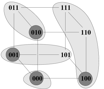
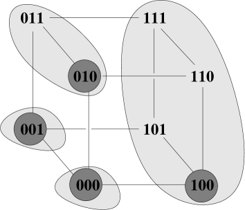
Figure 1: Binary code with four codewords 000, 100, 010, 001, with non-monotonic decoding (left) and monotonic decoding (right, discussed in Section 8). The light-grey sets indicate how a channel output is decoded.

Consider first the case that the receiver decodes the channel outputs $110,011,101$ as states $1,2,3$, respectively, that is, according to

$$d(110,1)=1,\quad d(011,2)=1,\quad d(101,3)=1.$$ (20)

We claim that this cannot be a Nash code, irrespective of the decoding probabilities $d(111,i)$ which can be positive for any $i=1,2,3$ by (19). The situation is symmetric for $i=1,2,3$, so assume that $d(111,i)$ is positive when $i=1$; the case of a deterministic decoding where $d(111,1)=1$ is shown on the left in Figure 1. Then the receiver decodes $y$ as state 1 with positive probability when $y$ equals $100$, $110$, or $111$. When $x^{1}=100$ is sent, these channel outputs are received with probabilities $(1-\varepsilon)^{3}$, $\varepsilon(1-\varepsilon)^{2}$, and $\varepsilon^{2}(1-\varepsilon)$, respectively, so the sender payoff is

$$(1-\varepsilon)^{3}+\varepsilon(1-\varepsilon)^{2}+\varepsilon^{2}(1-\varepsilon)\,d(111,1)$$

in (5). Given this decoding, the sender can improve her payoff in state 1 by sending $\hat{x}=110$ rather than $x^{1}=100$ because then the probabilities of the channel outputs $100$ and $110$ are just exchanged, whereas the probability that output $111$ is decoded as state 1 increases to $\varepsilon(1-\varepsilon)^{2}\,d(111,1)$; that is, given this decoding, sending $\hat{x}=110$ is more likely to be decoded correctly as state 1 than sending $x^{1}=100$. This violates (6).

The problem with the decoding in (20) is that when the receiver is tied between states 1, 2, and 3 when the channel output is $\hat{y}=111$, he decodes $\hat{y}$ as state 1 with positive probability $d(111,1)$, but when he is tied between even fewer states 1 and 3 when receiving $y=101$, that decoding probability $d(101,1)$ decreases to zero. This violates the following monotonicity condition.

Definition 5.1.

Consider a codebook with codewords $x^{i}$ for $i\in\Omega$. For a channel output $y$, let $T(y)$ be the set of tied states according to

$$T(y)=\{l\in\Omega\mid y\in Y_{l}\}.$$ (21)

Then a decoding function $d$ in $(\ref{dec})$ is called monotonic if it is a best response decoding function with $(\ref{Yi})$ and $(\ref{arbtie})$ and if for all $y,\hat{y}\in Y^{n}$ and states $i$,

$$i\in T(y)\subseteq T(\hat{y})~{}~{}\Rightarrow~{}~{}d(y,i)\geq d(\hat{y},i).$$ (22)

Furthermore, $d$ is called consistent if

$$i\in T(y)=T(\hat{y})~{}~{}\Rightarrow~{}~{}d(y,i)=d(\hat{y},i).$$ (23)

Condition (22) states that the probability of decoding the channel output as state $i$ can only decrease when the set of tied states increases. Condition (23) states that the decoding probability $d(y,i)$ of state $i$ may only depend on the set $T$ of states that are tied with $i$, but not on the received channel output $y$. Clearly, monotonicity implies consistency. We will show that for certain channels, in particular the binary channel, monotonic decoding gives a Nash code. However, for consistent decoding this is not the case. For example, the decoding shown in the left picture of Figure 1 is consistent because no two channel outputs have the same set of tied states, but the Nash property is violated.

Monotonic decoding functions exist, for example by breaking ties uniformly at random according to $d(y,i)=1/|T(y)|$ for $i\in T(y)$. We study the monotonicity condition in Definition 5.1 in more detail in later sections.

6 Nash codes for input symmetric channels

In this section, we state and prove our main result, Theorem 6.5 below, about binary codes. It turns out that it also applies to the following generalization of discrete channels where the error probability $\varepsilon_{y}$ of receiving an incorrect output symbol $y$ only depends on $y$ but not on the input.

Definition 6.1.

A discrete channel is input symmetric if $X=Y$ and there are errors $\varepsilon_{y}>0$ for $y\in Y$ so that $\sum_{y\in Y}\varepsilon_{y}<1$ and for all $x\in X$, $y\in Y$:

$$\begin{array}[]{rcll}p(y|x)&=&\varepsilon_{y}>0&\hbox{if }x\neq y,\\ p(y|x)&=&\nu_{y}>\varepsilon_{y}&\hbox{if }x=y,\\ \end{array}$$ (24)

where $\nu_{y}=1-\sum_{z\neq y}\varepsilon_{z}$ and thus for all $y$

$$\nu_{y}-\varepsilon_{y}=1-\sum_{z\in Y}\varepsilon_{z}>0\,.$$ (25)

Clearly, every binary channel is input symmetric. The matrix in (26) shows an example of an input symmetric channel with three symbols.

$$y$$

0 1 2

0 0.3 0.2 0.5

  1 0.1 0.4 0.5

2 0.1 0.2 0.7

(26)

By (25), the transition matrix of an input symmetric channel is the sum of a matrix where each row is identical (given by the errors) plus $\bigl{(}{1-\sum_{z\in Y}\varepsilon_{z}}\bigr{)}$ times the identity matrix. Definition 6.1 is chosen for our needs and, to our knowledge, not common in information theory; the definition of a symmetric channel by Cover and Thomas (1991, p. 190) is different, but covers the case where $\varepsilon_{y}=\varepsilon$ for all $y$.

A channel that is “output symmetric” is shown in (7), where for any given input $x$ the outputs $y$ other than $x$ have the same error probabilities $p(y|x)$. As we have shown with that example, such a channel may have codes that are not Nash codes.

The argument for Theorem 6.5 below rests on two lemmas. It is useful to partially order channel outputs and inputs by “closeness” to a given codeword as follows.

Definition 6.2.

Let $x,y,z\in S^{n}$ for some set $S$. Then $y$ is closer to $x$ than $z$ if and only if 

$$y_{j}\neq z_{j}~{}~{}\Rightarrow~{}~{}y_{j}=x_{j}\qquad\forall j=1,\ldots,n.$$

The following key lemma states in (29) that the decoding probability of a channel output $y$ for a state $i$ does not decrease when $y$ gets closer to the codeword $x^{i}$.

Lemma 6.3.

Consider a code for an input symmetric channel, a state $i$, channel outputs $y$ and $\hat{y}$, and assume $y$ is closer to codeword $x^{i}$ than $\hat{y}$. Then

$$i\in T(\hat{y})~{}~{}\Rightarrow~{}~{}i\in T(y)\,,$$ (27)

$$i\in T(\hat{y})~{}~{}\Rightarrow~{}~{}T(y)\subseteq T(\hat{y})\,,$$ (28)

and if the code is monotonically decoded then

$$d(y,i)\geq d(\hat{y},i).$$ (29)

Proof. To prove (27), we can assume that $y$ and $\hat{y}$ differ in only one symbol, because then (27) holds in general via a sequence of changes of only one symbol at a time. Assume that $y$ and $\hat{y}$ differ in the $j$th symbol, that is, $y_{j}\neq\hat{y}_{j}$ and $y_{-j}=\hat{y}_{-j}$ with the notation

$$y_{-j}=(y_{s})_{s\neq j},\quad y=(y_{j},y_{-j}).$$ (30)

With (1), we use the notation

$$p(y|x)=p(y_{j}|x_{j})\,p(y_{-j}|x_{-j}):=p(y_{j}|x_{j})\prod_{s\neq j}p(y_{s}|x_{s}),$$ (31)

and, for any $k$ in $\Omega$,

$$Q_{k}:=q_{k}V_{k}\,p(y_{-j}|x^{k}_{-j}).$$ (32)

Then by (3), $y\in Y_{i}$ means $q_{i}V_{i}\,p(y|x^{i})\geq q_{k}V_{k}\,p(y|x^{k})$ for all $k$ in $\Omega$, or equivalently

$$q_{i}V_{i}\,p(y_{j}|x^{i}_{j})\,p(y_{-j}|x^{i}_{-j})\geq q_{k}V_{k}\,p(y_{j}|x^{k}_{j})\,p(y_{-j}|x^{k}_{-j}),$$ (33)

that is, by (32), $y\in Y_{i}$ if and only if

$$\frac{p(y_{j}|x^{i}_{j})}{p(y_{j}|x^{k}_{j})}\geq\frac{Q_{k}}{Q_{i}}\qquad\forall k\in\Omega~{}.$$ (34)

Because $y$ is closer to $x^{i}$ than $\hat{y}$, we have $y_{j}=x^{i}_{j}\neq\hat{y}_{j}$. Suppose, to show (27), that $\hat{y}\in Y_{i}$, that is, because $y_{-j}=\hat{y}_{-j}$,

$$\frac{p(\hat{y}_{j}|x^{i}_{j})}{p(\hat{y}_{j}|x^{k}_{j})}\geq\frac{Q_{k}}{Q_{i}}\qquad\forall k\in\Omega~{},$$ (35)

and we want to show (34). For those $k$ where $x^{i}_{j}=x^{k}_{j}$, the left-hand side of (35) does not depend on $\hat{y}_{j}$ (and thus holds with $y_{j}$ instead of $\hat{y}_{j}$), so consider any state $k$ where $x^{i}_{j}\neq x^{k}_{j}$. Then by (24),

$$\frac{p(y_{j}|x^{i}_{j})}{p(y_{j}|x^{k}_{j})}=\frac{\nu_{y_{j}}}{\varepsilon_{y_{j}}}>1=\frac{\varepsilon_{\hat{y}_{j}}}{\varepsilon_{\hat{y}_{j}}}\geq\frac{p(\hat{y}_{j}|x^{i}_{j})}{p(\hat{y}_{j}|x^{k}_{j})}\geq\frac{Q_{k}}{Q_{i}}~{}\,$$ (36)

which shows (34). So $\hat{y}\in Y_{i}$ implies $y\in Y_{i}$, which proves (27).

To show (28), assume again that $y$ and $\hat{y}$ differ only in their $j$th symbol, and let $i\in T(\hat{y})$ and $l\in T(y)$ for a state $l$. That is, $\hat{y}\in Y_{i}$ and $y\in Y_{l}$, where $y\in Y_{i}$ by (27). Then states $i$ and $l$ are tied for $y$, and clearly

$$\frac{p(y_{j}|x^{i}_{j})}{p(y_{j}|x^{l}_{j})}=\frac{Q_{l}}{Q_{i}}\,.$$ (37)

If $x^{i}_{j}=x^{l}_{j}$ then (37) implies $Q_{l}=Q_{i}$ and (35) holds with $l$ instead of $i$, so $\hat{y}\in Y_{l}$, that is, $l\in T(\hat{y})$. If $x^{i}_{j}\neq x^{l}_{j}$, then the strict inequality (36) for $k=l$ contradicts (37), so this cannot be the case. This shows (28).

To show (29), assume monotonic decoding as in (22). If $\hat{y}\not\in Y_{i}$, then trivially $d(y,i)\geq d(\hat{y},i)=0$. Otherwise, $i\in T(\hat{y})$ and thus $i\in T(y)\subseteq T(\hat{y})$ by (27) and (28), which shows (29) by (22).     

The next lemma compares two channel inputs $x$ and $\hat{x}$ that differ in a single position $j$, and the corresponding channel output when that $j$th symbol arrives as $y_{j}$, for arbitrary other output symbols $y_{-j}$, using the notation (30).

Lemma 6.4.

Consider a monotonically decoded code for an input symmetric channel, and channel inputs $x$ and $\hat{x}$ which differ only in the $j$th symbol, where $x$ is closer to codeword $x^{i}$ than $\hat{x}$. Then for all $y_{-j}$

$$\sum_{y_{j}\in Y}p((y_{j},y_{-j})\,|\,x)~{}d((y_{j},y_{-j}),i)\geq\sum_{y_{j}\in Y}p((y_{j},y_{-j})\,|\,\hat{x})~{}d((y_{j},y_{-j}),i).$$ (38)

Proof. Because $x_{-j}=\hat{x}_{-j}$ and by (31), all terms in (38) have $p(y_{-j}|x_{-j})$ as a common factor. By taking that factor out and subtracting the right-hand side, (38) is equivalent to

$$\sum_{y_{j}\in Y}\bigl{(}p(y_{j}\,|\,x_{j})-p(y_{j}\,|\,\hat{x}_{j})\bigr{)}~{}d((y_{j},y_{-j}),i)\geq 0~{}.$$ (39)

If $y_{j}\neq x_{j}$ and $y_{j}\neq\hat{x}_{j}$, then $p(y_{j}\,|\,x_{j})-p(y_{j}\,|\,\hat{x}_{j})=\varepsilon_{y_{j}}-\varepsilon_{y_{j}}=0$, so (39) is equivalent to

$$\bigl{(}p(x_{j}\,|\,x_{j})-p(x_{j}\,|\,\hat{x}_{j})\bigr{)}~{}d((x_{j},y_{-j}),i)+\bigl{(}p(\hat{x}_{j}\,|\,x_{j})-p(\hat{x}_{j}\,|\,\hat{x}_{j})\bigr{)}~{}d((\hat{x}_{j},y_{-j}),i)\geq 0~{}.$$ (40)

By (25), $p(x_{j}\,|\,x_{j})-p(x_{j}\,|\,\hat{x}_{j})=\nu_{x_{j}}-\varepsilon_{x_{j}}=1-\sum_{z\in Y}\varepsilon_{z}=\nu_{\hat{x}_{j}}-\varepsilon_{\hat{x}_{j}}$, so that (40) is equivalent to

$$\Bigl{(}1-\sum_{z\in Y}\varepsilon_{z}\Bigr{)}\Bigl{(}d((x_{j},y_{-j}),i)-d((\hat{x}_{j},y_{-j}),i)\Bigr{)}\geq 0~{},$$ (41)

which is true because $d((x_{j},y_{-j}),i)=d((x_{j}^{i},y_{-j}),i)\geq d((\hat{x}_{j},y_{-j}),i)$ by (29). This shows (38).     

The following main theorem is essentially a corollary to Lemma 6.4.

Theorem 6.5.

Every monotonically decoded code for an input symmetric channel is a Nash code.

Proof. For any position $j$, a channel output $y$ is of the form $(y_{j},y_{-j})$ as considered in (38). If $x$ and $\hat{x}$ differ only in the $j$th position and $x$ is closer to $x^{i}$ than $\hat{x}$, with $x_{j}=x^{i}_{j}\neq\hat{x}_{j}$, then summing (38) over all $y_{-j}$ shows

$$\sum_{y\in Y^{n}}p(y|x)\,d(y,i)\geq\sum_{y\in Y^{n}}p(y|\hat{x})\,d(y,i)\,.$$

For an arbitrary channel input $\hat{x}$, considering one symbol at a time where $\hat{x}$ differs from $x^{i}$, this eventually gives (6), which proves the claim.     

In (34), it is used that all transition probabilities of the channel are positive. In fact, Theorem 6.5 does not hold without this assumption.

Remark 6.6.

If some error probabilities are zero, it is no longer true that every monotonically decoded binary code is a Nash code.

Proof. Consider a binary “Z-channel” where $p(1|0)=\varepsilon_{0}=0$ and $p(0|1)=\varepsilon_{1}=\varepsilon>0$, which is used twice ($n=2$), with transmission probabilities shown in (42).

$$\begin{array}[]{c|r|cccc|}\cline{2-6}\cr&&&\lx@intercol\hfil~{}~{}~{}y\hfil\lx@intercol&\\[-4.30554pt] \raise 8.61108pt\hbox{$q_{i}V_{i}$~{}}&\raise 8.61108pt\hbox{$p(y|x)$}&~{}~{}00{}{}&01&10&11\\ \cline{2-6}\cr 1&00&\framebox{1}&0&0&0\\ 1&01&\varepsilon&\framebox{$1-\varepsilon$}&\framebox{0}&\framebox{0}\\ &~{}\raise 10.76385pt\hbox{\smash{$x$}}\hfill 10&\varepsilon&0&1-\varepsilon&0\\ &11&\varepsilon^{2}&\varepsilon(1-\varepsilon)&(1-\varepsilon)\varepsilon&(1-\varepsilon)^{2}\\ \cline{2-6}\cr\end{array}$$ (42)

Assume uniform weights $q_{i}V_{i}=1$ and let the two codewords be $x^{0}=00$ and $x^{1}=01$, so that $Y_{0}=\{00,10,11\}$ and $Y_{1}=\{01,10,11\}$. Note that outputs 10 and 11 are both tied because they have probability zero with these inputs. Assume that these two “unobtainable” outputs are decoded as state 1, which defines a monotonic decoding rule (for a smaller set of tied states, the probability of decoding a state in the smaller set does not go down). This decoding is indicated by boxes in (42). However, this is not a Nash code because the sender can improve the probability of decoding state 1 from $1-\varepsilon$ to $1-\varepsilon^{2}$ by choosing $\hat{x}=11$ instead of $x^{0}=01$ as channel input.     

7 Nash-stable channels

In this section we carry the analysis of Section 6 one step further. This is motivated by Lemma 6.4 which asserts, in effect, that the Nash property applies when varying only the $j$th symbol in the transmitted $n$-tuple. That is, if a single use of the channel always gives a Nash equilibrium under monotonic decoding, then this also holds when the channel is used $n$ times independently, with codewords of length $n$. In fact, each of the $n$ times one can use a different channel. We first give a formal statement and proof of this observation. Afterwards, we discuss its relationship to the results of the previous section.

Definition 7.1.

A discrete noisy channel is called Nash-stable if, for a single use of the channel ($n=1$), every monotonically decoded code is a Nash code, for any number of states $i$ with nonnegative weights $q_{i}V_{i}$.

The following theorem considers a product of $n$ noisy channels with input and output alphabets $X{(j)}$ and $Y{(j)}$ and transition probabilities $p_{j}(y_{j}|x_{j})$ for $1\leq j\leq n$. These channels are used independently with channel inputs $x=(x_{1},\ldots,x_{n})$ and channel outputs $y=(y_{1},\ldots,y_{n})$, where $y$ is obtained, analogous to $(\ref{pyx})$, according to

$$p(y|x)=\prod_{j=1}^{n}p_{j}(y_{j}|x_{j}).$$ (43)

Note that the possible inputs $x$ to the product channel have their $n$ symbols distorted with independent errors, but the considered codes need not have any product structure. That is, the codewords can be chosen in any way just as in the previously considered case of using the same channel $n$ times.

Theorem 7.2.

The product of Nash-stable channels is Nash-stable.

Proof. Let $X=\prod_{j=1}^{n}X{(j)}$ and $Y=\prod_{j=1}^{n}Y{(j)}$. Consider a finite set $\Omega$ of states and a code $c:\Omega\to X$, where we denote the codewords by $x^{i}=c(i)$ as usual for $i$ in $\Omega$. Assume that the decoding function $d:Y\times\Omega\to{\mathbb{R}}$ is monotonic. If $c$ is not a Nash code, then there is some state $i$ and $x=x^{i}$ and $\hat{x}$ in $X$ so that

$$\sum_{y\in Y}p(y|x)\,d(y,i)<\sum_{y\in Y}p(y|\hat{x})\,d(y,i)\,.$$ (44)

As in Theorem 6.5, this implies that (44) holds for some $x$ and $\hat{x}$ in $X$ that differ only in their $j$th symbol with $x$ closer to $x^{i}$ than $\hat{x}$, that is, $x_{j}=x^{i}_{j}\neq\hat{x}_{j}$, and otherwise $x_{s}=\hat{x}_{s}$ for $s\neq j$, so we consider this case. Analogously to (31), we write $p(y|x)=p_{j}(y_{j}|x_{j})\,p(y_{-j}|x_{-j})$, and in addition let $Y_{-j}=\prod_{s\neq j}Y(s)$. Because $x_{-j}=\hat{x}_{-j}$, (44) is equivalent to

$$\sum_{y_{-j}\in Y_{-j}}p(y_{-j}|x_{-j})\sum_{y_{j}\in Y{(j)}}(p_{j}(y_{j}|x^{i}_{j})-p_{j}(y_{j}|\hat{x}_{j}))d((y_{j},y_{-j}),i)<0.$$

Hence, for at least one $y_{-j}$ we have $p(y_{-j}|x_{-j})>0$ and

$$\sum_{y_{j}\in Y{(j)}}p_{j}(y_{j}|x^{i}_{j})d((y_{j},y_{-j}),i)<\sum_{y_{j}\in Y{(j)}}p_{j}(y_{j}|\hat{x}_{j}))d((y_{j},y_{-j}),i).$$ (45)

(Apart from the notation $Y(j)$ for the output set of the $j$th channel, this just states that (39) does not hold.) We claim that (45) violates the assumption that the $j$th channel is Nash-stable. Namely, consider the same set of states $\Omega$ and the code $C:\Omega\to X(j)$ that encodes state $i$ as $C(i)=x^{i}_{j}$. The original full codeword $x^{i}=(x^{i}_{j},x^{i}_{-j})$ is sent across the product channel $X$, and the $j$th output symbol $y_{j}$ is decoded according to $D:Y{(j)}\times\Omega\to{\mathbb{R}}$ defined by

$$D(y_{j},i)=d((y_{j},y_{-j}),i)$$ (46)

for the fixed other outputs $y_{-j}$. We want that this reflects the original best-response decoding, which requires that the weights $q_{i}V_{i}$ are replaced by $q_{i}V_{i}\,p(y_{-j}|x^{i}_{-j})$ (which are exactly the weights $Q_{i}$ in (32)). Then we obtain the following division of $Y(j)$ into best-response sets $Y_{i}(j)$, analogous to (3):

$$Y_{i}(j)=\{y_{j}\in Y(j)\mid q_{i}V_{i}p(y_{-j}|x^{i}_{-j})\,p(y_{j}|x^{i}_{j})\geq q_{k}V_{k}p(y_{-j}|x^{k}_{-j})\,p(y_{j}|x^{k}_{j})~{}~{}\forall k\in\Omega\}.$$ (47)

Hence, $y_{j}\in Y_{i}(j)$ if and only if $(y_{j},y_{-j})\in Y_{i}$, which shows that $D$ in (46) is indeed a best-response decoding of the single-channel outputs $y_{j}$. Because $d$ is monotonic, so is $D$, because the tied states $l$ for $y_{j}$ (where $y_{j}\in Y_{l}(j))$) are those that are tied for $y=(y_{j},y_{-j})$ (where $y\in Y_{l}$). Because of (45), $(C,D)$ is not a Nash equilibrium and the $j$th channel is not Nash-stable as claimed. So $c$ is a Nash code for the product channel.     

Theorem 6.5 states that for an input symmetric channel that is used $n$ times independently, every code is a Nash code. In particular, it is a Nash code for $n=1$, so an input symmetric channel is Nash-stable. In addition, Theorem 7.2 is more general by allowing a different channel for each of the transmitted $n$ symbols, but it is straightforward to extend the proof of Theorem 6.5 to this case if each channel is input symmetric.

The condition of Nash-stability raises a number of questions. First, as the proof of Theorem 7.2 shows, a large number of states $i$ might be encoded with input symbols $x^{i}_{j}$ for the $j$th channel, with different weights $Q_{i}$, in order to use the assumption that the $j$th channel is Nash-stable. Does it matter if some of these weights $Q_{i}$ are zero? They are given by $Q_{i}=q_{i}V_{i}\,p(y_{-j}|x^{i}_{-j})$, so this happens when some channel error probabilities are zero. This case is not excluded in the definition of Nash-stability or in Theorem 7.2. However, such channels, for example the binary Z-channel, are not Nash-stable (which explains Remark 6.6), according to the following proposition. We do not consider the trivial case that $p(y|x)=0$ for all input symbols $x$, when the output symbol $y$ can be omitted altogether.

Proposition 7.3.

Consider a discrete noisy channel where for some input symbols $x$ and $\hat{x}$ and output symbol $y$ we have $p(y|x)=0$ and $p(y|\hat{x})>0$. Then this channel is not Nash-stable.

Proof. Consider $\Omega=\{0,1\}$, $q_{0}=q_{1}=1/2$, $V_{0}=2$, $V_{1}=1$, and the code $x^{0}=x^{1}=x$, so both states are mapped to the same channel input $x$ which cannot be received as channel output $y$. (This example can in fact be obtained from the proofs of Theorem 7.2 and Remark 6.6.) All outputs $y^{\prime}$ with $p(y^{\prime}|x)>0$ are decoded as the state 0 with higher weight. For the channel output $y$, both states are tied because this event has probability zero, so $y\in Y_{0}$. The receiver can therefore choose $d(y,1)=1$, that is, decode output $y$ as state 1, and decode all other outputs $\hat{y}$ so that $p(\hat{y}|x)=0$ as state 1 as well. This decoding is monotonic (the only sets of tied states are $\{0,1\}$ and $\{0\}$). Then in state 1, the sender can change from $x^{1}=x$ to $\hat{x}$ and increase the decoding probability from zero to at least $p(y|\hat{x})$. This improves her payoff, so the code is not a Nash code.     

The preceding remark shows that Nash-stability requires looking at “ambiguous” codes that map more than one state to the same codeword. However, it also shows that if all channel transmission probabilites are positive, then among any states mapped to the same channel input, only those with maximum weight can be decoded with positive probability. Clearly (as argued before in the proof of Proposition 3.1), “undecoded” states $i$ so that $d(y,i)=0$ for all $y$ can be ignored when checking Nash-stability. However, according to Definition 7.1, this still requires checking many conditions for the possible codes, weights, and monotonic decoding functions.

It can be shown, but is beyond the scope of this paper, that it is possible to restrict this check to deterministic monotonic decoding functions. Then no more than $|Y|$ states $i$ have the property that $d(y,i)>0$ for some $y$ in $Y$. For all other states, the Nash property holds trivially. For the weights for these states, there are only finitely many combinations of producing ties for any output $y$. The following remark illustrates this for a channel that is not input symmetric.

Remark 7.4.

There are Nash-stable channels that are not products of input symmetric channels.

Proof. Consider the following channel with three symbols.

$$y$$

0 1 2

0

  1

2

(48)

Consider deterministic monotonic decoding functions, where at most three states have positive probability of being decoded. If there is only one state decoded with positive probability, then the Nash condition holds trivially, and for three states it holds by Proposition 3.1. The symbols $0,1,2$ can be cyclically permuted without changing the channel, so suppose the code for two states $0$ and $1$ uses codewords $x^{0}=0$ and $x^{1}=1$. The decoding depends on the relative weights $q_{i}V_{i}$, so suppose priors are uniform and $V_{0}=1$. Then for $1/4<V_{1}<2$ we have $Y_{0}=\{0,2\}$ and $Y_{1}=\{1\}$, which gives a Nash code. If $V_{1}<1/4$ then $Y_{1}$ is empty and $Y_{0}=\{0,1,2\}$, which gives trivially a Nash code, and similarly if $V_{1}>2$. If $V_{1}=1/4$, then $Y_{0}=\{0,1,2\}$ and $Y_{1}=\{1\}$, and the two states are tied for $y=1$. If output $y=1$ is decoded as state 0, then the Nash property holds trivially, if as state 1, then sending $x^{1}$ gives the maximum decoding probability $4/7$, so this is also a Nash code.

If $V_{1}=2$, then $Y_{0}=\{0,2\}$ and $Y_{1}=\{0,1,2\}$, so that the two states are tied both for $y=0$ and $y=2$. By consistency, both outputs $y=0$ and $y=2$ are decoded either as state 0 or as state 1, which correspond to the cases already considered and give Nash codes.

Finally, it is not hard to see that any mixed decoding strategy that is monotonic is a convex combination of the considered deterministic monotonic decoding functions, which implies the Nash property as well. This applies also to many states where more than one state is mapped to the same input symbol.     

The computational difficulty of deciding if a given channel is Nash-stable is open. The problem belongs to the complexity class co-NP because it is is easy to verify that the channel is not Nash-stable, by providing suitable weights, a code, a monotonic decoding function, and a profitable deviation. We envisage two possible answers: Either one can show that Nash-stable channels require that multiple ties occur simultaneously, like for input symmetric channels or in the example (48), and check only codes with few states. In that case, there may be a polynomial-time algorithm. Alternatively, the problem whether a channel is Nash-stable may be co-NP-complete. We leave this as a topic for future research.

8 General deterministic monotonic decoding functions

When is a deterministic decoding function monotonic? Suppose there is some fixed order on the set of states so that always the first tied state is chosen according to that order. In this final section, we show that this is essentially the only way to break ties with a deterministic monotonic decoding function if it is defined for all sets of tied states $T$ with up to three states.

Because any monotonic decoding function is consistent according to (23), it is useful to consider it as a function $d:\mathcal{T}\times\Omega\to{\mathbb{R}}$ where

$$T\in\mathcal{T}\quad\Leftrightarrow\quad T=T(y)=\{l\in\Omega\mid y\in Y_{l}\}\quad\hbox{for some }y\in Y$$ (49)

and

$$d(T,i):=d(y,i)\quad\hbox{if }T=T(y)$$ (50)

which is well defined by (23). Whether we write $d(T,i)$ or $d(y,i)$ will be clear from the context.

Consider again the example (20) with $d(111,1)=1$ as shown on the left in Figure 1. The following decoding function, changed from (20) so that $101$ is decoded as state 1, is monotonic,

$$d(110,1)=1,\quad d(011,2)=1,\quad d(101,1)=1,\quad d(111,1)=1,$$ (51)

shown in the right picture in Figure 1. This is a Nash code because all $y$ in the set $Y_{1}$, see (19), are decoded as state 1; whichever $\hat{x}$ in $Y_{1}$ the sender decides to transmit instead of $x^{1}$, there is one $y$ in $Y_{1}$ for which $p(y|\hat{x})=\varepsilon^{2}(1-\varepsilon)$, so that the payoff to the sender in (5) does not increase by changing from $x^{1}$ to $\hat{x}$.

As the right picture in Figure 1 shows, the decoding function in (51) can be defined by the following condition: Consider a fixed linear order $\prec$ on $\Omega$ (in this case $0\prec 1\prec 2\prec 3$) so that

$$d(T,i)=1~{}~{}~{}\Leftrightarrow~{}~{}~{}i\in T~{}\hbox{ and }~{}\forall k\in T,~{}k\neq i~{}:~{}i\prec k\,.$$ (52)

That is, the decoding rule chooses the $\prec$-smallest state $i$ from the set $T$. A fixed-order decoding function $d$ fulfills (52) for some $\prec$. Such a decoding function is deterministic and clearly monotonic.

We want to show that any deterministic monotonic decoding function is a fixed-order decoding function. We have to make the additional assumption that the decoding function $d(T,i)$ is general in the sense that it is defined for any nonempty set $T$ (where it suffices to require this at least for all $|T|\leq 3$), not only the sets $T$ in $\mathcal{T}$ that occur as sets of tied states for some channel output $y$ as in (49).

Without this assumption, we could add to the above example another state with codeword $x^{4}=111$ so that the “circular” decoding function in (20) is monotonic and gives a Nash code, but is clearly not a fixed-order decoding function. It is reasonable to require that a decoding function is defined generally and does not just coincidentally lead to a Nash code because certain ties do not occur (as argued above, with the decoding (20) we do not have a Nash code when ties have to be resolved for $y=111$).

For general decoding functions, the monotonicity condition (22) translates to the requirement that for any $T,\hat{T}\subseteq\Omega$,

$$i\in T\subseteq\hat{T}~{}~{}\Rightarrow~{}~{}d(T,i)\geq d(\hat{T},i).$$ (53)

Proposition 8.1.

Suppose that $d(T,i)$ is deterministic and defined for all nonempty sets $T$ with $|T|\leq 3$ (for example, if $\mathcal{T}$ in $(\ref{calT})$ contains all these sets) and fulfills $(\ref{genmono})$. Then $d$ is a fixed-order decoding function.

Proof. Define the following binary relation $\prec$ on $\Omega$:

$$i\,\prec\,k~{}~{}~{}\Leftrightarrow~{}~{}~{}d(\{i,k\},i)=1.$$

Clearly, either $i\,\prec\,k$ or $k\,\prec\,i$ for any two states $i,k$. We claim that $\prec$ is transitive, that is, if $i\,\prec\,k$ and $k\,\prec\,l$, then $i\,\prec\,l$. Otherwise, there would be a “cycle” of distinct $i,k,l$ with $i\,\prec\,k$ and $k\,\prec\,l$ and $l\,\prec\,i$. This is symmetric in $i,k,l$, so assume $d(\{i,k,l\},i)=1$ and therefore $d(\{i,k,l\},k)=0$ and $d(\{i,k,l\},l)=0$. However, with $T=\{i,l\}$ and $\hat{T}=\{i,k,l\}$ we have $d(T,i)=0<1=d(\hat{T},i)$, which contradicts (53).

So $\prec$ defines a linear order on $\Omega$. We show that (52) holds, that is, for any $\hat{T}$ in $\mathcal{T}$ the decoded state $i$ (so that $d(\hat{T},i)=1$) is the $\prec$-smallest element of $\hat{T}$. This holds trivially and by definition if $\hat{T}$ has at most two elements, otherwise, if $l\,\prec\,i$ for some $l\in\hat{T}$, then we obtain with $T=\{i,l\}$ the same contradiction $d(T,i)=0<1=d(\hat{T},i)$ as before. So the decoded state is chosen according to the fixed order $\prec$ on $\Omega$ as claimed.     

When the weights $q_{i}V_{i}$ for the states $i$ are generic, then $Y_{i}$ in (3) is always a singleton, so no ties occur and decoding is deterministic. One can make any weights generic by perturbing them minimally so that ties are broken uniquely but decoding is otherwise unaffected. That is, if $i$ and $k$ are tied for some $y$ because $q_{i}V_{i}\,p(y|x^{i})=q_{k}V_{k}\,p(y|x^{k})$, this tie is broken in favor of $i$ by slightly increasing $q_{i}V_{i}$, which will then always happen whenever $i$ and $k$ are tied originally. This induces a fixed-order decoding, where any linear order among the states can be chosen. Thus, Proposition 8.1 asserts that general deterministic monotonic decoding functions are those obtained by generic perturbation of the weights.

Finally, we observe that the above codebook $000,100,010,001$ with decoding as in (51) defines a Nash code (and if priors are minimally perturbed so that $q_{1}>q_{2}>q_{3}$ there are no ties and decoding is unique), but this code is not locally optimal as in Theorem 4.4. Namely, by changing the codeword $100$ to $110$, all possible channel outputs $y$ differ in at most one bit from one of the four codewords, which clearly improves the payoff to the receiver. So not all binary Nash codes are locally receiver-optimal.

References

Anshelevich, E., et al. (2008), The price of stability for network design with fair cost allocation. SIAM Journal on Computing 38, 1602–1623.

Argiento R., R. Pemantle, B. Skyrms, and S. Volkov (2009), Learning to signal: Analysis of a micro-level reinforcement model. Stochastic Processes and their Applications 119, 373–390.

Blume, A., and O. J. Board (2013), Intentional vagueness. Erkenntnis, DOI 10.1007/s10670-013-9468-x, 45 pages.

Blume, A., O. J. Board, and K. Kawamura (2007), Noisy talk. Theoretical Economics 2, 395–440.

Cover, T. M., and J. A. Thomas (1991), Elements of Information Theory. Wiley, New York.

Crawford, V., and J. Sobel (1982), Strategic information transmission. Econometrica 50, 1431–1451.

De Jaegher, K., and R. van Rooij (2013), Game-theoretic pragmatics under conflicting and common interests. Erkenntnis, DOI 10.1007/s10670-013-9465-0, 52 pages.

Gallager, R. G. (1968), Information Theory and Reliable Communication. Wiley, New York.

Glazer, J., and A. Rubinstein (2004), On optimal rules of persuasion. Econometrica 72, 1715–1736.

Glazer, J., and A. Rubinstein (2006), A study in the pragmatics of persuasion: A game theoretical approach. Theoretical Economics 1, 395–410.

Hernández, P., A. Urbano, and J. E. Vila (2010), Nash equilibrium and information transmission coding and decoding rules. Discussion Papers in Economic Behaviour ERI-CES 09/2010, University of Valencia.

Hernández, P., A. Urbano, and J. E. Vila (2012), Pragmatic languages with universal grammars. Games and Economic Behavior 76, 738–752.

Jäger, G., L. Koch-Metzger, and F. Riedel (2011), Voronoi languages: Equilibria in cheap talk games with high-dimensional types and few signals. Games and Economic Behavior 73, 517–537.

Kamenica, E., and M. Gentzkow (2011), Bayesian persuasion. American Economic Review 101, 2590–2615.

Koessler, F. (2001), Common knowledge and consensus with noisy communication. Mathematical Social Sciences 42, 139–159.

Kreps, D. M., and J. Sobel (1994), Signalling. In: R. J. Aumann and S. Hart, eds., Handbook of Game Theory with Economic Applications, Vol. 2, Elsevier, Amsterdam, 849–867.

Lewis, D. (1969), Convention: A Philosophical Study. Harvard University Press, Cambridge, MA.

Lipman, B. (2009), Why is language vague? Mimeo, Boston University.

MacKay, D. J. C. (2003), Information Theory, Inference, and Learning Algorithms. Cambridge University Press, Cambridge, UK.

MacKenzie, A. B., and L. A. DaSilva (2006), Game Theory for Wireless Engineers. Morgan and Claypool.

Monderer, D., and L. S. Shapley (1996), Potential games. Games and Economic Behavior 14, 124–143.

Myerson, R. B. (1994), Communication, correlated equilibria and incentive compatibility. In: R. J. Aumann and S. Hart, eds., Handbook of Game Theory with Economic Applications, Vol. 2, Elsevier, Amsterdam, 827–847.

Nowak, M., and D. Krakauer (1999), The evolution of language. Proc. Nat. Acad. Sci. USA 96, 8028–8033.

Pawlowitsch, C. (2008), Why evolution does not always lead to an optimal signaling system. Games and Economic Behavior 63, 203–226.

Shannon, C. E. (1948), A mathematical theory of communication. Bell System Technical Journal 27, 379–423; 623–656.

Sobel, J. (2012), Complexity versus conflict in communication. Proc. 46th Annual Conference on Information Sciences and Systems (CISS). DOI 10.1109/CISS.2012.6310777, 6 pages.

Sobel, J. (2013), Giving and receiving advice. In: Advances in Economics and Econometrics, Tenth World Congress of the Econometric Society, D. Acemoglu, M. Arellano and E. Dekel (eds.), Cambridge University Press.

Spence, M. (1973), Job market signaling. The Quarterly Journal of Economics 87, 355–374.

Srivastava, V., et al. (2005), Using game theory to analyze wireless ad hoc networks. IEEE Communications Surveys and Tutorials 7, Issue 4, 46–56.

Touri, B., and C. Lambort (2013), Language evolution in a noisy environment. Proc. American Control Conference (ACC), 1938–1943.

Wärneryd, K. (1993), Cheap talk, coordination and evolutionary stability. Games and Economic Behavior 5, 532–546.