Long-range 1D gravitational-like interaction in a neutral atomic cold gas

Abstract

A quasi-resonant laser induces a long-range attractive force within a cloud of cold atoms. We take advantage of this force to build in the laboratory a system of particles with a one-dimensional gravitational-like interaction, at a fluid level of modeling. We give experimental evidences of such an interaction in a cold Strontium gas, studying the density profile of the cloud, its size as a function of the number of atoms, and its breathing oscillations.

I Introduction

When interactions between the microscopic components of a system act on a length scale comparable to the size of the system, one may call them “long-range”: For instance, the inverse-square law of the gravitational force between two point masses which is one of the most celebrated and oldest laws in physics. In the many particles world, it is responsible for dramatic collective effects such as the gravothermal catastrophe Antonov (1961) or the gravitational clustering which is the main mechanism leading to the formation of the structure of galaxies in the present universe. Beyond gravitation, such long-range interactions are present in various physical fields, either as fundamental or as effective interactions: In plasma physics Elskens and Escande (2002), two dimensional (2D) fluid dynamics reffluid , degenerated quantum gases O’Dell et al. (2000), ion trapping Porras and Cirac (2004), to cite only these works. long-range interactions deeply influence the dynamical and thermodynamical properties of such systems. At the thermodynamic equilibrium, long-range interactions are at the origin of very peculiar properties, especially for attractive systems: The specific heat may be negative; canonical (fixed temperature) and microcanonical (fixed energy) ensembles are not equivalent. These special features have been known for a long time in the astrophysics community, in the context of self gravitating systems.

After the seminal works of Lynden-Bell and Wood Lynden-Bell and Wood (1968) and Thirring Thirring (1970), many contributions followed on this subject (see, for instance, Campa et al. (2009) for a recent review), so that the equilibrium characteristics of attractive long-range interacting systems are theoretically well established. This situation is in striking contrast with the experimental side of the problem: There is currently no controllable experimental system exhibiting the predicted peculiarities. There have been some proposals to remedy to this situation: O’Dell et al. O’Dell et al. (2000) have suggested creating an effective $1/r$ potential between atoms in a Bose-Einstein condensate using off-resonant laser beams; more recently, Dominguez et al. Dominguez et al. (2010) have proposed taking advantage of the capillary interactions between colloids to mimic two-dimensional gravity, and Golestanian Golestanian (2012) has suggested experiments using thermally driven colloids. However, these proposals have not been implemented yet, and so far the dream of a tabletop galaxy remains elusive.

The key results of this paper are to show some experimental evidences of a gravitational-like interaction in a quasi-one-dimensional (hereafter 1D) test system consisting in a cold gas of Strontium atoms in interaction with two contra-propagating quasi-resonant lasers. To our knowledge, it is the first experimental realization of the 1D gravitational toy model, which can be compared with the theoretical predictions developed for more than $50$ years by the astrophysical and statistical physics community. In the stationary regime, the cloud spatial distribution is in agreement with the well-known $\mbox{sech}^{2}$ law for the 1D self-gravitating gas at thermal equilibrium Camm (1950). Moreover, the long-range attractive nature of the force is confirmed studying the cloud’s size dependency as a function of the number of atoms. Out of equilibrium, the breathing oscillation frequency increases with the strength of the interaction as it should be for attractive interactions. Quantitatively our experimental results are in agreement with the expected $1/r^{\alpha}$ force with $\alpha=0$.

The paper is organized as follows. In Sec. II, we start from the radiation pressure exerted by the lasers and explain under which circumstances this force becomes analog to a 1D gravitational force. We then make some definite theoretical predictions on the size, density profile, and oscillation frequency of the interacting atomic cloud. The experimental setup is described in Sec. III. In the same section, the experimental results are compared with the theory.

II Model and theoretical predictions

The gravitational potential $U(r)$ between two particles can be expressed through the Poisson equation $\nabla^{2}U(\mathbf{r})=A_{D}Gm\delta(\mathbf{r})$, where $G$ is the coupling constant, $m$ the mass of the particle and $A_{D}$ a numerical constant which depends on the dimension. The solution of the Poisson equation for the interpaticle potential $U(r)$ in three dimension is the well-known

$$U(r)=\frac{Gm}{r},$$ (1)

and in 1D,

$$U(r)=Gm|r|$$ (2)

(for a review on 1D gravitational systems see, e.g., Yawn and Miller (2003)). After using a mean-field approach (see below), we will show that such a potential should be at play in our experiment, under precise circumstances (see section II.2).

We start considering a quasi-1D $\{$cold atomic gas + 1D quasi-resonant laser beams$\}$ system; an atomic gas, with a linear density $n(z)$, is in interaction with two contra-propagating laser beams. The two beam intensities $I_{+}(z)$ and $I_{-}(z)$, where $I_{+}(-\infty)=I_{-}(+\infty)\equiv I_{0}$, respectively propagating in the positive and negative direction, are much smaller than the atomic line saturation intensity $I_{s}$. Thus the atomic dipolar response is linear. The radiation pressure force of the lasers on an atom, having a longitudinal velocity $v_{z}$, is given by Metcalf and van der Straten (1994):

$$F_{\pm}(z,v_{z})=\pm\hbar k\frac{\Gamma}{2}\frac{\Gamma^{2}}{4(\delta\mp kv_{z})^{2}+\Gamma^{2}}\frac{I_{\pm}(z)}{I_{s}},$$ (3)

where $\hbar$ is the reduced Planck constant, $\Gamma$ the bare linewidth of the atomic transition, $k$ the wave number, and $\delta$ the frequency detuning between an atom at rest and the lasers. For a cloud of $N$ atoms, the attenuation of the laser intensity is given by:

$$\textrm{d}I_{\pm}=\mp\frac{\sigma_{\pm}}{2\pi L_{\perp}^{2}}NI_{\pm}n(z)\textrm{d}z,$$ (4)

where $n(z)$ is the normalized linear density profile and

$$\sigma_{\pm}=\frac{6\pi}{k^{2}}\Gamma^{2}\int\frac{g(v_{z})}{4(\delta\mp kv_{z})^{2}+\Gamma^{2}}\textrm{d}v_{z}$$ (5)

is the average absorption cross-section for a single atom. $g(v_{z})$ is the normalized longitudinal velocity distribution and $2\pi L_{\perp}^{2}$ is the transverse section of the cloud. At equilibrium $g(v_{z})$ is an even function so $\sigma_{-}=\sigma_{+}\equiv\sigma$. The optical depth is defined as:

$$b=\frac{\sigma}{2\pi L_{\perp}^{2}}N\int_{-\infty}^{+\infty}n(z)\textrm{d}z=\frac{\sigma N}{2\pi L_{\perp}^{2}}\,.$$ (6)

Atoms also experience a velocity diffusion due to the random photon absorptions and spontaneous emissions: This is modeled by a velocity diffusion coefficient $D$ introduced in Eq. (7). In experiments, $\delta<0$ such that the force, given in Eq. (3), is a cooling force counteracting the velocity diffusion. We now describe the $N$ atoms by their phase space density in 1D, $f(z,v_{z},t)$. As in Verkerk (2011), we write a Vlasov Fokker-Planck equation

$$\begin{split}\frac{\partial f}{\partial t}+v_{z}\frac{\partial f}{\partial z}&-\omega_{z}^{2}z\frac{\partial f}{\partial v_{z}}+\frac{1}{m}\frac{\partial}{\partial v_{z}}[(F_{+}(z,v_{z})+F_{-}(z,v_{z}))f]\\ &=D\frac{\partial^{2}f}{\partial v_{z}^{2}}.\end{split}$$ (7)

which is, for most of the cases, a reasonable modeling of long-range force systems in the mean-field approximation (see, e.g., Binney and Tremaine (2008)). The second term in Eq. (7) is an inertial one, whereas the third one describes a harmonic trapping force being a good approximation of the dipolar trap used in the experiment Chu et al. (1986). Indeed the dipolar potential, in the longitudinal axe of interest, can be written as

$$U_{dip}(z)=\frac{-U_{0}}{1+\left(\frac{z}{z_{R}}\right)^{2}}$$ (8)

with $z_{R}=1.2$ mm, $U_{0}=\frac{1}{2}k_{B}T_{\mathrm{trap}}$, and $T_{\mathrm{trap}}=20\mu K$. The observed rms longitudinal size being $L_{z}\lesssim 400\mu m$, it is reasonable to perform a Taylor expansion around $z=0$ to get the harmonic approximation:

$$U_{dip}(z)\approx-U_{0}\left[1-\left(\frac{z}{z_{R}}\right)^{2}\right].$$ (9)

having a characteristic frequency

$$\omega_{z}=\left(\frac{k_{B}T_{\mathrm{trap}}}{mz_{R}^{2}}\right)^{1/2}.$$ (10)

The fourth term of Eq. (7) contains the mean-field force $F_{\pm}$ divided by the atomic mass $m$. The right hand side describes a velocity diffusion. The use of a one dimensional model is justified by the fact that the ratio between the rms transverse $L_{\perp}$ and longitudinal $L_{z}$ size of the cloud measured in the experiment is $L_{\perp}/L_{z}\approx 2\times 10^{-2}$. Eq. (7) neglects atomic losses and dependencies in position and velocity of the velocity diffusion coefficient.

One notes that the attractive force coming from the beams absorption (Eq. (3) and (4)) is known since the early days of laser cooling and trapping Dalibard (1988). However, in an usual 3D setting this attractive force is dominated by the repulsive force due to photons reabsorption Walker et al. (1990), which, in the small optical depth limit, may be seen as an effective repulsive Coulomb force. By contrast, in a 1D configuration with an elongated cloud along the cooling laser beams, the probability of photons reabsorption is reduced by a factor of the order of $L_{\perp}/L_{z}$, in comparison with the isotropic cloud having the same longitudinal optical depth. In our experiment, the reduction factor is about $2\times 10^{-2}$, so that the repulsive force can be safely ignored. Similar but weaker reduction of the probability of photons reabsorption is also expected for the 2D geometry, which opens the possibility of experimental systems analogous to 2D self-gravitating systems.

II.1 Fluid approximation

In order to solve Eq. (7) we assume that the system can be described using a fluid approach: The velocity distribution at time $t$ does not depend on the position, except for a macroscopic velocity $u(z,t)$. We write then the one point distribution function $f$ as

$$f(z,v_{z},t)=mNn(z,t)\frac{1}{\Delta(t)}g\left(\frac{v_{z}-u(z,t)}{\Delta(t)}\right).$$ (11)

The velocity distribution $g(v_{z})$ is even, centered around $u$; the velocity dispersion is characterized by a time modulation $\Delta(t)$. Integrating Eq. (7) over $dv_{z}$ and over $v_{z}~{}dv_{z}$, we obtain the fluid equations:

$$\frac{\partial n}{\partial t}+\frac{\partial}{\partial z}\left(nu\right)=0\quad$$ (12)

$$\frac{\partial(nu)}{\partial t}+\frac{\partial}{\partial z}\left[\left(u^{2}+\Delta(t)^{2}\int v_{z}^{2}g(v_{z})dv_{z}\right)n\right]+\omega_{z}^{2}zn$$

$$-\frac{1}{m}n\int(F_{+}+F_{-})g\left(\frac{v_{z}-u(z,t)}{\Delta(t)}\right){\Delta(t)}dv_{z}=0.\quad$$ (13)

II.2 Stationary solution

We first look for a stationary solution; this imposes $u=0$ and $\Delta=1$. Eq. (12) is then automatically satisfied; Eq. (13) for the stationary density $n(z)$ reads:

$$\bar{v}_{z}^{2}\frac{\partial n}{\partial z}+\omega_{z}^{2}zn-\frac{1}{m}n\int[F_{+}+F_{-}]g(v_{z})dv_{z} = 0\,,$$ (14)

where we have used the notation $\int v_{z}^{2}g(v_{z})dv_{z}=\bar{v}_{z}^{2}$.

Eq. (4) is easily integrated, yielding:

$$I_{+}(z) = I_{0}e^{-b\int_{-\infty}^{z}n(s)ds}$$ (15)

$$I_{-}(z) = I_{0}e^{-b\int_{z}^{+\infty}n(s)ds}$$ (16)

The exponentials are expanded up to first order, according to the small optical depth hypothesis $b\ll 1$:

$$I_{+}(z) \simeq I_{0}\left(1-b\int_{-\infty}^{z}n(s)ds\right)$$ (17)

$$I_{-}(z) \simeq I_{0}\left(1-b\int_{z}^{+\infty}n(s)ds\right)~{}.$$ (18)

Introducing these expressions for $I_{\pm}$ into Eq. (14), we obtain finally

$$\bar{v}_{z}^{2}\frac{\partial n}{\partial z}+\omega_{z}^{2}zn-NCn\int_{-\infty}^{+\infty}\mbox{sgn}(s-z)n(s)ds=0\,,$$ (19)

where

$$C=\frac{3\hbar\Gamma}{2mkL_{\perp}^{2}}\frac{I_{0}}{I_{s}}\left(\sigma\frac{k^{2}}{6\pi}\right)^{2}~{}.$$ (20)

Eq. (19) is equivalent to an equation describing the stationary density of an assembly of $N$ trapped particles of mass $m$, with gravitational coupling constant $G$, in an external harmonic trap of frequency $\omega_{z}$, in a heat bath at temperature $T$, with the correspondence:

$$\bar{v}_{z}^{2} \leftrightarrow\frac{k_{B}T}{m}$$ (21a)

$$C \leftrightarrow Gm~{},$$ (21b)

where $k_{B}$ is the Boltzmann constant. Two characteristic lengths are identified;

$$L_{ni}=\sqrt{\frac{k_{B}T}{m\omega_{z}^{2}}}$$ (22)

is the characteristic size of the non-interacting gas in its external harmonic holding potential. Using Eq. (10) we get

$$L_{ni}=\sqrt{\frac{T}{T_{trap}}}z_{R}.$$ (23)

The other characteristic length $L_{i}$ is associated with the interaction strength:

$$L_{i}=\frac{k_{B}T}{NCm}.$$ (24)

Using these notations we write Eq. (19) as

$$\frac{\partial n}{\partial z}+\frac{zn}{L_{ni}^{2}}-\frac{n}{L_{i}}\int_{-\infty}^{+\infty}\mbox{sgn}(s-z)n(s)ds=0~{}.$$ (25)

The first term of (25) favors the density spreading. In contrast with the 2D and 3D cases, it always prevents the collapse of the cloud Padmanabhan (1990). The second term describes an external harmonic confinement coming from the dipole trap in the experiment. The third term is the attractive interaction due to laser beams absorption. It corresponds to an 1D gravitational potential expresses in Eq. (2). If the inequality $L_{i}\ll L_{ni}$ is fulfilled, Eq. (25) is the one expected for a 1D self-gravitating gas at thermal equilibrium Camm (1950). It yields the profile:

$$n(z)=\frac{1}{4L_{i}}\textrm{sech}^{2}\left(\frac{z}{2L_{i}}\right).$$ (26)

A generalization of Eq. (25) is written as:

$$\frac{\partial n}{\partial z}+\frac{1}{k_{B}T}\frac{\partial U_{dip}}{\partial z}n-An\int_{-\infty}^{+\infty}|s-z|^{-\alpha}\mbox{sgn}(s-z)n(s)ds=0~{},$$ (27)

including the exact form of the dipole trap (8), and the variation of the interaction exponent $\alpha$ of a $1/r^{\alpha}$ attractive force. This expression is used to compare theory with experiments in section III. $A$ is a free parameter controlling the interaction strength, and thus the width of the equilibrium profile.

II.3 Breathing oscillations

To probe the dynamics of the system, we now go back to Eqs. (12,13), linearizing these equations with respect to $u$ and $\Delta-1$: For small amplitude oscillations. One notes that this approximation is much less restrictive than linearizing with respect to the velocity $v_{z}$. We then compute $\int[F_{+}+F_{-}]fdv_{z}$:

$$\begin{split}\int[F_{+}+F_{-}]fdv_{z}\simeq&~{}c_{1}(I_{+}-I_{-})n+c_{2}(I_{+}+I_{-})nu\\ &+c_{3}(\Delta-1)(I_{+}-I_{-})n~{},\end{split}$$ (28)

where the constants $c_{i}$ involve integrations with respect to $v_{z}$. The first term is the gravitational-like force, as in (19) with $n(z)$ replaced by the time-dependent density $n(z,t)$. The second one is a friction, which a priori depends weakly on $z$ through $I_{+}+I_{-}$. Since $I_{+}-I_{-}$ is of order $b\ll 1$, the third term, of order $b(\Delta-1)$, is neglected. We assume that the dynamics is captured by a single parameter $\lambda(t)$, using the ansatz Olivetti et al. (2009):

$$f(z,v_{z},t)=mNn(z/\lambda)g(\lambda v_{z}-\dot{\lambda}z).$$ (29)

When compared with (11), this amounts to assume: $u=\frac{\dot{\lambda}}{\lambda}z,~{}\Delta=1/\lambda$. We introduce the notations $\langle.\rangle$ and $\langle.\rangle_{0}$ for the spatial average of a quantity over the density at time $t$ and the stationary density respectively. Then

$$\langle z^{2}\rangle=\lambda^{2}\langle z^{2}\rangle_{0}~{},~{}\langle zu\rangle=\lambda\dot{\lambda}\langle z^{2}\rangle_{0}~{},~{}\langle u^{2}\rangle=\dot{\lambda}^{2}\langle z^{2}\rangle_{0}~{}.$$ (30)

We note that Eq. (12) is automatically satisfied by the ansatz (29). To obtain an equation for $\lambda$, we integrate Eq. (13) over $z~{}dz$. We obtain, for $\lambda$ close to $1$ (small amplitude oscillations):

$$\ddot{\lambda}+\kappa\dot{\lambda}+\omega^{2}(\lambda-1)=0$$ (31)

with $\kappa$ an effective friction and a breathing oscillation frequency:

$$\omega_{\textrm{br}}=\omega_{z}\left(3(p-1)+4\right)^{\frac{1}{2}}~{}.$$ (32)

$p$ measures the compression of the cloud:

$$p=\frac{L_{ni}^{2}}{L_{z}^{2}}.$$ (33)

In experiments where the effective friction is rather small, Eq. (32) is expected to be a fair approximation for the breathing oscillation frequency. More generally, assuming a power law two-body interaction force in the gas $1/r^{\alpha}$, the simple relation for $\omega_{\textrm{br}}$ in the weak damping limit becomes Olivetti et al. (2009):

$$\omega_{\textrm{br}}=\omega_{z}\left((3-\alpha)(p-1)+4\right)^{\frac{1}{2}}.$$ (34)

This formula relates $\omega_{\textrm{br}}$ to $\alpha$ and $p$, and will be used in section III.4. Eq. (34) was derived in Olivetti et al. (2009) assuming a velocity independent interaction term, which would be obtained by linearizing the radiation pressure force (3) in velocity. This is not a reasonable approximation in our experiments Olivetti et al. (2012), but we have shown here that (34) is still expected to provide a reasonable approximation for the breathing frequency in the limit of small optical depth.

III Experiments

III.1 Experimental setup

The sample preparation is done in the same way as depicted in Chalony et al. (2011). More details about laser cooling of Strontium in a magneto-optical trap (MOT) can be found in Chaneliere et al. (2008). After laser cooling, around $10^{5}$ atoms at $T\simeq 3\,\mu$K are loaded into a far detuned dipole trap made of a $120$ mW single focused laser beam at $780$ nm. Analysis are performed using in-situ images taken with a CCD at different instant of the experimental sequence. The longitudinal profile is obtained averaging over the irrelevant remaining transverse dimension. We directly measure the longitudinal trap frequency $\omega_{z}=6.7(0.5)$ Hz from relaxation oscillations of the cold cloud (see example of temporal evolutions in Fig. 1). The radial trap frequency $\omega_{\perp}=470(80)$Hz is deduced from cloud size measurements. The beam waist is estimated at $23(2)\,\mu$m leading to a potential depth of $T_{\textrm{trap}}\simeq 20\,\mu$K.

$50$ ms after loading the dipole trap (corresponding to $t=0$ in Fig. 1), a contra-propagating pair of laser beams, red-detuned with respect to the ${}^{1}\!S_{0}\rightarrow\,^{3}\!P_{1}$ intercombination line at $689$ nm (radiative lifetime: $21\,\mu$s), is turned on for $400$ ms. These beams, aligned with respect to the longitudinal axis of the cloud, generate the effective 1D attractive interaction. When the 1D lasers are on, we apply a $B=0.3$ G magnetic bias field, for two important reasons: First, the Zeeman degeneracy of the excited state is lifted such that the lasers interact only with a two-level system made out of the $m=0\rightarrow m=0$ transition which is insensitive to the residual magnetic field fluctuation. Second, the orientation of magnetic field bias, with respect to the linear polarization of the dipole trap beam, is tuned to cancel the clock (or transition) shift induced by the dipole trap on the transition of interest Chalony et al. (2011).

The temperature along the 1D laser beams, in our experimental runs, is found to be in the range of $1-3\,\mu$K. Even at such low temperatures, and in sharp contrast with standard broad transitions, the frequency Doppler broadening $k\bar{v}_{z}$ remains larger than $\Gamma$. As a direct consequence, the optical depth $b$ depends on the exact longitudinal velocity distribution $g(v_{z})$ (see Eqs. (5) and (6)) which are not necessarily gaussian Chalony et al. (2011). Since we measure only the second moment of the distribution $g(v_{z})$, namely: $\bar{v}_{z}$ or $T$, one has enough control to assert the $b\ll 1$ limit, thus the occurrence of the self-gravity regime. However we can perform only qualitative tests of our theory described in section II.2.

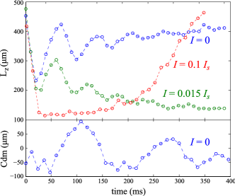
Figure 1: Upper part: (Color online) Typical temporal evolutions of $L_{z}$ the rms longitudinal size of the atomic cloud for three different 1D beam intensities. The laser detuning is $\delta=-5\Gamma$ for all curves. Lower part: The center of mass (Cdm) position of the atomic gas without the 1D lasers ($I=0$). The $y$ axis origin is arbitrary.

At $t=-50$ms, the MOT cooling laser beams are turned off, leaving the trapped atomic cloud in an out-of-equilibrium macroscopic state. Without the 1D lasers, we observed a weakly damped oscillation of the breathing mode and of the center of mass position (blue circles in Fig. 1). One notes that damping is caused by anharmonicity of the dipole trap and not by thermalization of the gas which is negligible on the experimental timescale. In presence of the 1D laser beams, overdamped or underdamped oscillations of the cloud are observed.

III.2 Stationary state’s density profile

Let us first consider the stationary state in the overdamped situation (red circles in Fig. 1). After the transient phase ($t<30$ ms), the rms longitudinal size of the atomic gas reaches a plateau at a minimal value of $L_{z}\simeq 120\,\mu$m with $T\simeq 2\,\mu$K. The slow increase of the cloud’s size after the plateau ($t>150$ ms) goes with an increase of the temperature up to $4\,\mu$K at the end of the time sequence. The origins of the long time scale evolution are not clearly identified, but it is most likely due to coupling of the longitudinal axis with the uncooled transverse dimensions because of imperfect alignment of the 1D laser beams with the longitudinal axis of the trap and nonlinearities of the trapping forces. At the plateau where temperature is around $2\,\mu$K the non-interacting gas is expected to have a rms longitudinal size of $L_{z}=L_{ni}\simeq 370\,\mu$m. Hence, a clear compression of the gas by a factor of three is observed. It is due to the attractive interaction induced by the absorption of the 1D laser beams. Moreover, the estimated optical depth is $b<0.6$. We then approach the two previously mentioned conditions — $b\ll 1$ and $L_{z}\ll L_{ni}$ — for being in the 1D self-gravitating regime as discussed in section II.2. In Fig. 2, where $b\simeq 0.4$, we test the effective interaction in the gas by assuming a power law two-body interaction force in the gas $1/r^{\alpha}$ and fitting the experimental linear density distribution for different values of $\alpha$ in the presence of a dipolar trap; $\alpha=0$ corresponds to 1D gravity. We see that the best fit seems to be for $\alpha\in[0,1/2]$.

In absence of the 1D laser beams, we have checked that the experimental linear density distribution have the expected profile of a non interacting gas in our dipole trap having a $z_{R}=1.2(1)$ mm Rayleigh length.

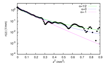
Figure 2: (Color online) Density linear distribution for $N=10^{5}$. The black circles are the experimental data with $I=0.02I_{s}$, $\delta=-6\Gamma$ and $b\simeq 0.4$. The profiles were symmetrized to improve the signal to noise ratio. The curves are least square fits of the data using Eq. (27) containing the exact form of the dipole trap and a two-body interaction force $1/r^{\alpha}$. The fits are performed for each $\alpha$ by fixing the normalization and varying the interaction strength.

III.3 Cloud’s longitudinal size

In the self-gravitating regime a $1/N$ dependency of $L_{z}$ is expected at fixed temperature (see (26) and the definition of $L_{i}$). Fig. 3 shows that the cloud’s size $L_{z}$ is in agreement with this prediction for two temperature ranges: $1.5(2)\,\mu$K (blue circle) and $2.1(2)\,\mu$K (red star). Fits correspond to the blue dashed line for $1.5(2)\,\mu$K and the red dashed line for $2.1(2)\,\mu$K. The fitting expression is

$$N=a(1/L_{z}-L_{z}/L_{ni}^{2})\,,$$ (35)

where $a$ and $L_{ni}$ are free parameters depending on the temperature of the gas. If $L_{ni}\gg L_{z}$, the self-gravitating regime is recovered in the fitting expression. However Eq. (35) takes into account the presence of a harmonic trap. Eq. (35) can be simply derived using the generalized virial theorem (see Eq. (11) in Ref. Werner (2008)) and it is in perfect agreement with numerical integrations of Eq. (25). The fits give $L_{ni}\simeq 0.5$ mm, slightly larger than the expected value of $L_{ni}$ at these temperatures. The $1/N$ dependency of $L_{z}$ in the self-gravitational regime is consistent with a long-range interaction with $\alpha=0$. Unfortunately as discussed above, the residual Doppler effect prevents a quantitative comparison with the prediction of our model.

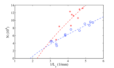
Figure 3: (Color online) Dependency of the longitudinal size of the cloud with the number of atoms for $\delta=5.7(5)\Gamma$ and $I=0.3I_{s}$. The blue circle (red star) data points correspond to temperature $1.5(2)\,\mu$K ($2.1(2)\,\mu$K). The optical depth is in the range of 0.6-0.2 according to atoms number variations. The blue and the red dashed lines are fits using Eq. (35).

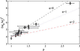
Figure 4: (Color online) Comparison for $\alpha=0,1$ and $2$ of the experimental ratio $(\omega_{\textrm{br}}/\omega_{z})^{2}$ and the predictions deduced from the relation (34). The values of $p$ are measured on the experiment.

III.4 Breathing oscillations

Let us now consider the evolution of the trapped cold cloud in the underdamped situation (as an example see green circles in Fig. 1). Without the 1D lasers, the ratio of the eigenfrequencies of the breathing mode $\omega_{\textrm{br}}$ and the center of mass $\omega_{z}$ is found to be close to two, as expected for a non-interacting gas in a harmonic trap. As an example the blue curve, shown in Fig. 1, gives $\omega_{\textrm{br}}/\omega_{z}=1.9(1)$. If now the attractive long-range interaction is turned on, $\omega_{\textrm{br}}$ is expected to follow Eq. (34) whereas $\omega_{z}$ should remain unchanged.

Fig. 4 summarizes the comparisons between the measured ratio $(\omega_{\textrm{br}}/\omega_{z})^{2}$ and the predictions deduced from the relation (34). $p$ is computed from the experimental data in the stationary state. We expect $\alpha=0$, however to judge the nature of the long-range attractive interaction, three plots respectively for $\alpha=0,~{}1$ and $2$ are shown. If the $\alpha=2$ case can be excluded, the experimental uncertainties does not allow to clearly discriminate between $\alpha=0$ and $\alpha=1$. In conjunction with Fig. 2, we conclude that the system is reasonably well described by a gravitational-like interaction, $\alpha=0$.

IV Conclusion and perspectives

In this paper, we give strong indications of an 1D gravitational-like interaction in a Strontium cold gas induced by quasi resonant contra-propagating laser beams. First, we show that in the self-gravitating limit, the density distribution follows the theoretically expected profile. Moreover, the scaling of the cloud size with the number of atoms follows the predicted $1/N$ law. Finally, the modification of breathing frequency of the cloud, due to the long-range interaction, is correctly described by a self-gravitating model.

Other phenomena can also be investigated e.g. in relation with plasma physic; Landau damping should be observed studying the return to equilibrium of the system after various perturbations. Moreover, the actual experimental system could be easily extended to 2D geometry suggesting interesting consequences: By contrast with the 1D case, a 2D self-gravitating fluid undergoes a collapse at low enough temperature, or strong enough interaction. Hence, it is conceivable that an experiment similar to the one presented in this paper, in a pancake geometry, would show such a collapse Barré, Wilkowski, Marcos (2012).

Acknowledgements: This work is partially supported by the ANR-09-JCJC-009401 INTERLOP project. DW wishes to thank Frédéric Chevy for fruitful discussions.

References

- Antonov (1961) V. Antonov, Soviet Astr.-AJ 4, 859 (1961).
- Elskens and Escande (2002) Y. Elskens, and D. Escande, Microscopic Dynamics of Plasmas and Chaos (IOP Publishing, Bristol, 2002).
- (3) P.H. Chavanis, in Dynamics and Thermodynamics of Systems with Long-Range Interactions, Eds. T. Dauxois, S. Ruffo, E. Arimondo and M. Wilkens, Springer (2002).
- O’Dell et al. (2000) D. O’Dell, S. Giovanazzi, G. Kurizki, and V. M. Akulin, Phys. Rev. Lett. 84, 5687 (2000).
- Porras and Cirac (2004) D. Porras, and J.I. Cirac, Phys. Rev. Lett. 92, 207901 (2004).
- Lynden-Bell and Wood (1968) D. Lynden-Bell and R. Wood, M. Not. Roy. Astron. Soc. 138, 495 (1968).
- Thirring (1970) W. Thirring, Zeitschrift für Physik A 235, 339 (1970).
- Campa et al. (2009) A. Campa, T. Dauxois, and S. Ruffo, Phys. Rep. 480, 57 (2009).
- Dominguez et al. (2010) A. Dominguez, M. Oettel, and S. Dietrich, Phys. Rev. E 82, 11402 (2010).
- Golestanian (2012) R. Golestanian, Phys. Rev. Lett. 108, 038303 (2012).
- Camm (1950) G. Camm, M. Not. Roy. Astron. Soc. 110, 305 (1950).
- Yawn and Miller (2003) K. R. Yawn, and B. N. Miller, Phys. Rev. E 68, 056120 (2003).
- Metcalf and van der Straten (1994) H. Metcalf and P. van der Straten, Phys. Rep. 244, 203 (1994).
- Verkerk (2011) R. Romain, D. Hennequin, and P. Verkerk, Eur. Phys. J. D. 61, 171-180 (2011).
- Binney and Tremaine (2008) J. Binney and S. Tremaine, Galactic Dynamics (Princeton University Press, 2008).
- Chu et al. (1986) S. Chu, J.E. Bjorkholm, and A. Ashkin, A. Cable, Phys. Rev. Lett. 57, 314 (1986).
- Dalibard (1988) J. Dalibard, Opt. Comm. 68, 203 (1988).
- Walker et al. (1990) T. Walker, D. Sesko, and C. Wieman, Phys. Rev. Lett. 64, 408 (1990).
- Padmanabhan (1990) T. Padmanabhan Phys. Rep. 188, 285 (1990).
- Olivetti et al. (2009) A. Olivetti, J. Barré, B. Marcos, F. Bouchet, and R. Kaiser, Phys. Rev. Lett. 103, 224301 (2009).
- Olivetti et al. (2012) For our experimental data points shown in Fig. 4, .
- Chalony et al. (2011) M. Chalony, A. Kastberg, B. Klappauf, and D. Wilkowski, Phys. Rev. Lett. 107, 243002 (2011).
- Chaneliere et al. (2008) T. Chaneliere, L. He, R. Kaiser, and D. Wilkowski, Eur. Phys. J. D 46, 507 (2008).
- Werner (2008) F. Werner, Phys. Rev. A 78, 025601 (2008).
- Barré, Wilkowski, Marcos (2012) J. Barré, D. Wilkowski, and B. Marcos, in preparation.