State engineering of Bose-Einstein condensate in the optical lattice by a periodic sublattice of dissipative sites

Abstract

We introduce the notion of dissipative periodic lattice as an optical lattice with periodically distributed dissipative sites and argue that it allows to engineer unconventional Bose-Einstein superfluids with the complex-valued order parameter. We consider two examples, the one-dimensional dissipative optical lattice, where each third site is dissipative, and the dissipative honeycomb optical lattice, where each dissipative lattice site neighbors three non-dissipated sites. The tight-binding approximation is employed, which allows one to obtain analytical results. In the one-dimensional case the condensate is driven to a coherent Bloch-like state with non-zero quasimomentum, which breaks the translational periodicity of the dissipative lattice. In the two-dimensional case the condensate is driven to a zero quasimomentum Bloch-like state, which is a coherent superposition of four-site discrete vortices of alternating vorticity with the vortex centers located at the dissipative sites.

I Introduction

Bose-Einstein condensates (BEC) in the optical lattices have become an universal laboratory to study various quantum phenomena of the condensed matter physics PS ; JZ ; MO ; Bloch . A spectacular achievement in this direction is the demonstrated single-site addressability of the two-dimensional optical lattices ContRem1 ; ContRem2 , i.e. the atoms can be controllably removed from the lattice sites selected at will. Another intriguing recent development is observation of the unconventional boson superfluidity in the higher bands of the optical lattice Pbos ; Fbos ; SpinBos , described by a complex-valued order parameter and, therefore, beyond the no-node theorem of R. Feynman (see for instance, the review Wu ).

The purpose of the present paper is to demonstrate that the single-site addressability in the optical lattices allows one to generate the unconventional boson superfluids. To this goal, one can use the controlled removal of atoms by the technique of Refs. ContRem1 ; ContRem2 from a periodic sublattice of the optical lattice with BEC loaded in it. It is shown below that the condensate is driven to a coherent non-local Bloch-like state described by a complex-valued order parameter (in the two-dimensional case) or the order parameter with nodes (in the one-dimensional case). This is achieved by the emulation of a coherent non-local dissipation by a local one, similar as in the recently proposed scheme for generators of the non-classical states of photons MS ; QSG .

The quantum state engineering based on the dynamics in the open quantum systems QSEQC , in particular in the optical lattices QSE , is a well-known idea. As distinct from the previous proposal of the quantum state engineering in the optical lattices (see also the recent study DrDissLatt ), where the inter-site atomic currents are coupled to reservoirs, in our case the dissipation acts locally and incoherently on a periodic sublattice of the lattice sites, whereas the condensate is driven to a non-local coherent state.

It is known that the action of dissipation in conjunction with the nonlinearity can increase coherence of the quantum state of BEC. For instance, the possibility to engineer the order parameter of BEC by a localized dissipative perturbation (i.e. by a dissipative defect) was shown in Ref. BKPO . It was also shown that the quantum coherence of a strongly interacting BEC loaded in the double-well trap subject to the phase noise and particle loss can be completely restored by engineering the parameters of the system and controlling the dissipation rate WTW1 . Similar results were obtained with the optical lattices, where the particle loss at the boundary acting together with the nonlinearity resulted in restoration of the coherence and formation of the discrete breathers WTW2 . Whereas in the previous setups the action of a localized or boundary dissipation was considered, in the present proposal we consider the action of a periodic dissipation which profoundly affects the physics in the optical lattice. Therefore, to distinguish such a setup from the usual optical lattice, it will be called below the dissipative lattice. Indeed, a strong periodic dissipation effectively changes the lattice space group, it results in a bigger unit cell for the dissipative lattice as compared to the same lattice without the periodic dissipation. The dissipative lattice can have both the dissipative as well as the (almost) non-dissipative coherent modes, which are Fourier-like expansions over some superpositions of the local modes in each unit cell. The long-term state of BEC in the dissipative lattice is a lowest energy subset of the effective dark states, i.e. the states almost unaffected by the dissipation as the result of the quantum Zeno effect QZ ; CPZeno (see also the reviews ZRew1 ; ZRew2 ). Finally, in contrast to the previous works, a weak nonlinearity in our case plays only an auxiliary role (see the honeycomb lattice example below), which is to break the energy degeneracy of the effective dark states and select one particular state.

The paper is arranged as follows. In section II we consider the simple case of the one-dimensional periodic dissipative lattice, where the action of a periodically distributed dissipative sites is discussed. Then, in section III, we consider a more involved case of a dissipative honeycomb optical lattice. Section IV contains the discussion of the main results and a general perspective on the dissipative periodic lattices.

II The one-dimensional lattice with a periodic sublattice of dissipative sites

Here we consider the simplest case of one-dimensional dissipative lattice to illustrate the main idea. Specifically, we concentrate on the one-dimensional lattice where each third lattice site is dissipative with the same dissipative rate, see Fig. 1. The selected periodicity of the dissipative sites is the most dense one within the class of the dissipative sublattices which still allow for the non-dissipative coherent modes in the unit cell (see Fig. 1(a)). We consider the tight-binding approximation with the nearest neighbor tunneling and a weak nonlinearity as compared to the tunneling and dissipation rates. Then the standard boson Hubbard Hamiltonian applies, which in the notations of Fig. 1(a) reads

$$H=-J\sum_{n}\{a^{\dagger}_{n,0}(a_{n,-}+a_{n,+})+a^{\dagger}_{n,+}a_{n+1,-}+\textrm{h.c.}\}$$

$$+\frac{U}{2}\sum_{n}\{(a^{\dagger}_{n,-})^{2}a^{2}_{n,-}+(a^{\dagger}_{n,0})^{2}a^{2}_{n,0}+(a^{\dagger}_{n,+})^{2}a^{2}_{n,+}\},$$ (1)

where the index $n$ enumerates the unit cells of the dissipative lattice. Note that the dissipative lattice period is ${\bf D}=3{\bf d}$, where ${\bf d}$ is the period of the original (non-dissipative) lattice.

We assume that the atoms are removed with a constant and uniform rate $\Gamma$ from the sublattice of sites as indicated in Fig. 1, which can be realized, for example, by the technique of Refs. ContRem1 ; ContRem2 . Then, the state of the system is given by the density matrix $\rho$ satisfying the quantum master equation in the Lindblad form (see, for more details, Ref. NlZeno and Ref. Book for a general discussion)

$$\frac{d\rho}{dt}=-\frac{i}{\hbar}[H,\rho]+\Gamma\sum_{n}\mathcal{D}\left[a_{n,0}\right]\rho,$$ (2)

where the Lindblad term is defined as $\mathcal{D}[a]\rho\equiv a\rho a^{\dagger}-\frac{1}{2}[a^{\dagger}a\rho+\rho a^{\dagger}a]$.

The reason to use a larger unit cell of the lattice in Eq. (1) and (2) is that, for a strong dissipation rate, the population of the dissipative sites is locked to that of the non-dissipative ones (see Ref. ThreeSite for further details) and can be adiabatically eliminated. In this way, the problem of finding the ground state of BEC in the dissipative lattice is reduced to that of a modified non-dissipative lattice, where the boson operators in each unit cell are some coherent modes over the non-dissipative sites ($c_{n,\pm}$ below). Our use of the introduced notion of the dissipative periodic lattice leads to a significant reduction of complexity of the analytical analysis.

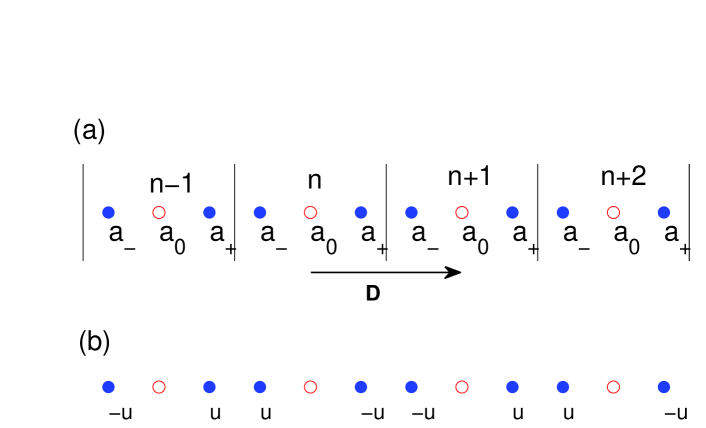
Figure 1: (Color online) (a) A schematic depiction of the one-dimensional lattice with a periodic sublattice of dissipative sites (open circles). The lattice unit cell selection is shown by vertical lines, where in each unit cell the lattice sites are enumerated by “$-$”, “$0$” and “$+$” (shown by the subscript to the local boson operator $a$). The consequential numbers on top enumerate the unit cells and the vector labelled by ${\bf D}$ at the bottom is the dissipative lattice period. (b) Schematic depiction of the Bloch mode $\varphi_{\frac{L}{2},-}$. Here $u=\frac{1}{\sqrt{2L}}$.

We focus on the limit of strong dissipation $\Gamma\gg J/\hbar$ and neglect the nonlinearity assuming it to be too weak to have contribution on the considered time scale. Specifically, we assume the condition $J/(\hbar\Gamma)\gg U\langle{a^{\dagger}a}\rangle/J\,$ where $\langle a^{\dagger}a\rangle$ is the average atomic filling of the non-dissipative wells. By performing the adiabatic elimination of the dissipative sites ($a_{n,0}$) (for the details, consult Ref. QSG , section II) the master equation is reduced to that for the non-dissipative sites only (with the reduced density matrix $\rho_{R}$), which is in the same form as Eq. (2) with, however, a reduced dissipation rate $\gamma$ and a reduced Hamiltonian $H_{R}$ (the terms depending on the operators of the dissipative sites are thrown away). The coupling to the dissipative sites in Eq. (1) suggests to define the coherent modes in each unit cell as follows $c_{n,\pm}=(a_{n,+}\pm a_{n,-})/\sqrt{2}$, then the tunneling part of the reduced Hamiltonian becomes

$$H_{R} = \frac{J}{4}\sum_{n}\{c^{\dagger}_{n,-}c_{n+1,-}-c^{\dagger}_{n,+}c_{n+1,+}+\mathrm{h.c.}\}$$ (3)

$$+ \frac{J}{2}\sum_{n}\{c^{\dagger}_{n,+}(c_{n+1,-}-c_{n-1,-})+\mathrm{h.c.}\}.$$

Since only mode $c_{n,+}$ is coupled directly (with the coupling coefficient $\sqrt{2}J$) to the dissipative mode $a_{n,0}$ in each unit cell, the reduced master equation reads (Ref. QSG , section II)

$$\frac{d\rho_{R}}{dt}=-\frac{i}{\hbar}[H_{R},\rho_{R}]+\gamma\sum_{n}\mathcal{D}\left[c_{n,+}\right]\rho_{R},\quad\gamma\equiv\frac{8J^{2}}{\hbar^{2}\Gamma}.$$ (4)

For the times staring from $t\sim 1/\gamma$ the state of the system is defined by the global coherent modes which are decoupled from the dissipative modes. Indeed, let us define the coherent lattice modes (which can be called the dissipative Bloch modes) as follows

$$\varphi_{k,\pm}=\frac{1}{\sqrt{L}}\sum_{n}e^{\frac{2\pi i}{L}kn}c_{n,\pm},$$ (5)

where $L$ is the total number of unit cells (i.e. $L=N/3$ where $N$ is the number of lattice sites, see Fig. 1). The unitary transformation (5) leaves the Lindblad term in the master equation (4) invariant, i.e. Eq. (4) has the same form in the Bloch basis

$$\frac{d\rho_{R}}{dt}=-\frac{i}{\hbar}[H_{R},\rho_{R}]+\gamma\sum_{n}\mathcal{D}\left[\varphi_{n,+}\right]\rho_{R}.$$ (6)

Eq. (6) defines a subspace of the dark states, which consists of the Bloch modes decoupled from the dissipative modes $\varphi_{k,+}$. To find such modes we rewrite the Hamiltonian (3) in the Bloch basis

$$H_{R}=\frac{J}{2}\sum_{k}\cos\left(\frac{2\pi}{L}k\right)(\varphi^{\dagger}_{k,-}\varphi_{k,-}-\varphi^{\dagger}_{k,+}\varphi_{k,+})$$

$$+J\sum_{k}\left\{i\sin\left(\frac{2\pi}{L}k\right)\varphi^{\dagger}_{k,-}\varphi_{k,+}+\mathrm{h.c.}\right\}.$$ (7)

It is seen that the dark subspace contains two Bloch modes $\varphi_{0,-}$ and $\varphi_{\frac{L}{2},-}$ (more precisely, the Bloch modes with $\delta\equiv(k-k_{d})/L\ll 1\,$, for $k_{d}=0$ or $k=L/2$, have significantly reduced decay rate due to weak coupling to the dissipative modes, since the coupling coefficient reads $J|\sin\left(\frac{2\pi}{L}k\right)|\approx J|\delta|$). Moreover, since the dissipative lattice modes $\varphi_{k,-}$ have a negative kinetic energy, see Eq. (7), the lowest energy mode is the Bloch mode $\varphi_{\frac{L}{2},-}$. Note that the long-term ground state $\varphi_{\frac{L}{2},-}$ breaks the discrete translational symmetry of the dissipative lattice (the translation by ${\bf D}$), since in terms of the local basis we have

$$\varphi_{\frac{L}{2},-}=\frac{1}{\sqrt{2L}}\sum_{n}(-1)^{n}(a_{n,+}-a_{n,-}),$$ (8)

which is schematically depicted in Fig. 1(b).

Let us summarize the main conclusions of this simple example. The dissipative optical lattice with a strong dissipation rate is effectively equivalent to an effective non-dissipative lattice, which has unusual properties of the long-term ground state of BEC. In this particular case the effectively negative kinetic energy of the non-dissipative sublattice results in the Bloch state with a non-zero quasimomentum, which breaks the translational symmetry of the dissipative lattice. Below we consider a more intriguing example of two-dimensional lattice, where the sublattice of the dissipative sites induces a long-term state of BEC with a vortex-like phase distribution.

III The honeycomb optical lattice with a periodic sublattice of dissipative sites

Let us now consider the lattice with the hexagonal symmetry, namely, the honeycomb optical lattice. The specific choice of the lattice has two reasons. First, in the tight-binding limit, the honeycomb lattice reduces to just four nearest-neighbor sites with equal tunneling amplitude, where three sites are arranged in the form of an equilateral triangle and one more cite is placed at its center, see Fig. 2(a). From this perspective, by application of the external dissipation to the central cite in each such triangle one arranges for the three non-dissipated sites coupled to it, thus the next possible number as compared to the one-dimensional case considered in section II. Second, within the class of two-dimensional lattices, the lattices with the hexagonal symmetry are known for their intriguing properties, such as the appearance of the Dirac cones (i.e. the Dirac Hamiltonian) in the Bloch band intersections and the related topological phase transitions Latt2 ; IntDirCone , including the phase transition from the conventional to unconventional superfluidity SpinBos . Thus, one naturally expects the dissipative honeycomb lattice to possess an interesting long-term ground state.

The simplest honeycomb optical lattice, which was experimentally realized Latt1 , is created by intersection of three laser beams of of the same frequency and equal intensities. When the lasers are blue detuned from the atomic transition frequency, the lattice minima are at the vertices of honeycombs. In this case, the optical lattice potential reads $V({\bf x})=V_{0}\sum_{j=1}^{3}\cos({\bf b}_{j}{\bf x})$, where ${\bf x}=(x,y)$, ${\bf b}_{1,2}$ are the basis vectors of the reciprocal lattice, with ${\bf b}_{2}$ being the vector ${\bf b}_{1}$ rotated by $\pi/3$, and ${\bf b}_{3}={\bf b}_{2}-{\bf b}_{1}$. We note that, interestingly, the following lattice

$$V=8V_{0}\sin^{2}\left(\frac{{\bf b}_{1}{\bf x}}{2}\right)\sin^{2}\left(\frac{{\bf b}_{2}{\bf x}}{2}\right)\sin^{2}\left(\frac{{\bf b}_{3}{\bf x}}{2}\right),$$ (9)

shown in Fig. 2(a), has also the honeycomb shape, but possesses much more pronounced minima of the lattice wells (it can be realized with the recent optical lattice technology Latt3 , see also Ref. OptExpr ). The results obtained below, however, apply to any of the optical lattices reducible in the tight-binding limit to the honeycomb arrangement of the lattice wells, where in each equilateral triangle there are three non-dissipated sites located at the vertices and the dissipative site located at the center, i.e. as in Fig. 2.

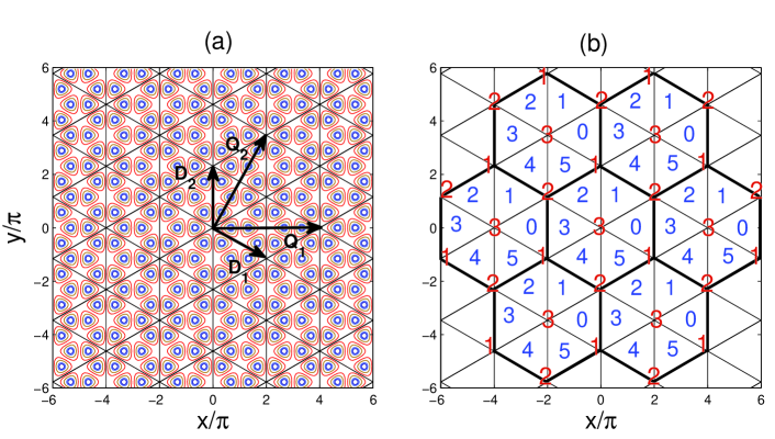
Figure 2: (Color online) (a) Contour plot of the honeycomb optical lattice (9) (the lattice minima are shown). The dissipative sites are located at the centers of the four-site elementary triangles (shown here by the division lines). The vectors ${\bf D}_{1,2}$ give the basis of the dissipative lattice periods, whereas ${\bf Q}_{1,2}$ connect the equivalent hexagons (shown by the thick lines in panel (b)). (b) Division of the dissipative lattice into the set of the equivalent hexagons used for representation of the Hamiltonian. The numbers at the vertices give the indices of the local boson operators corresponding to the non-dissipative wells, while the inner numbers enumerate the triangles inside each equivalent hexagon.

Taking into account the discussion of section II, we will use from the start the nomenclature defined by the dissipative lattice, see Fig. 2(b). In particular, the lattice wells are enumerated as shown in Fig. 2, where each elementary triangle (shown by the thin lines in Fig. 2(a)) contains one dissipative lattice well at the center, to which we assign the boson annihilation operator $a_{0}$, and three non-dissipative wells at the vertices, with the corresponding operators $a_{1,2,3}$, as is schematically shown in Fig. 2(b). It is seen that the dissipative lattice periods are given as ${\bf D}_{1}=\frac{8\pi}{3|{\bf b}|^{2}}(2{\bf b}_{1}-{\bf b}_{2})$ and ${\bf D}_{2}=\frac{8\pi}{3|{\bf b}|^{2}}(2{\bf b}_{2}-{\bf b}_{1})$ (which are twice the original honeycomb lattice periods). It proves convenient to use the equivalent hexagons shown by the thick lines in Fig. 2(b) as the unit cells of the dissipative lattice (see below). Therefore, we introduce the basis of the translations ${\bf Q}_{1}=2{\bf D}_{1}+{\bf D}_{2}$ and ${\bf Q}_{2}=2{\bf D}_{2}+{\bf D}_{1}$, Fig. 2(a), which translate the equivalent hexagons into each other without any change in the enumeration of the lattice wells. The annihilation operator at a given lattice site now is denoted by $a_{{\bf q},n,l}$, where $l=0,1,2,3$ is the lattice site index inside the triangle, $n\in\{0,\ldots,5\}$ is the triangle index and ${\bf q}=q_{1}{\bf Q}_{1}+q_{2}{\bf Q}_{2}$, $q_{j}\in\{0,\pm 1,\pm 2,\ldots\}$, is the hexagon index.

Our division of the hexagonal lattice into the equivalent hexagons, as in Fig. 2(b), and the specific enumeration scheme are dictated by the geometry of the strongly dissipative sublattice. Though the indices of the local operators assigned to the non-dissipative sites in each hexagon still can be distributed at will, the selected enumeration shown in Fig. 2(b) proves to be the most convenient.

In the tight-binding limit with the nearest-neighbor tunneling confined to the lowest Bloch band, the boson Hubbard Hamiltonian reads

$$H=-J\sum_{\langle{,}\rangle}(a^{\dagger}_{{\bf q},n,k}a_{{\bf q}^{\prime},m,l}+\textrm{h.c.})+\frac{U}{2}\sum_{{\bf q},n,k}(a^{\dagger}_{{\bf q},n,k})^{2}a^{2}_{{\bf q},n,k},$$ (10)

where the first sum is over the nearest neighbors and $U$ is the nonlinear interaction strength proportional to the $s$-wave scattering length of BEC.

We assume that the standard Markovian dissipation with the constant and spatially uniform rate $\Gamma$ is applied to the lattice wells located at the centers of the elementary triangles of Fig. 2. Then the master equation reads

$$\frac{d\rho}{dt}=-\frac{i}{\hbar}[H,\rho]+\Gamma\sum_{{\bf q}}\sum_{n=0}^{5}\mathcal{D}\left[a_{{\bf q},n,0}\right]\rho.$$ (11)

In the limit of strong dissipation, i.e.

$$\Gamma\gg\frac{J}{\hbar},\qquad\Gamma\gg\frac{U\langle{a^{\dagger}a}\rangle}{\hbar},$$ (12)

the dissipative wells can be adiabatically eliminated, thus reducing the master equation (11) to that for the non-dissipative wells only. Skipping the details (see Ref. QSG , section II), let us write down the resulting reduced master equation for the density matrix $\rho_{R}$ describing the non-dissipative sites

$$\frac{d\rho_{R}}{dt}=-\frac{i}{\hbar}[H_{R},\rho_{R}]+\mathcal{L}\rho_{R},\quad\mathcal{L}\rho_{R}=\gamma\sum_{{\bf q}}\sum_{n=0}^{5}\mathcal{D}[c_{{\bf q},n,3}]\rho_{R},$$ (13)

where the reduced rate reads $\gamma={12J^{2}}/({\hbar^{2}\Gamma})$, $H\equiv H_{R}$ is the reduced Hamiltonian (the part of $H$ from Eq. (9) dependent only on $a_{{\bf q},n,l}$ and $a^{\dagger}_{{\bf q},n,l}$ with $l=1,2,3$) and the local coherent basis used in the representation of Eq. (13) is defined by the unitary transformation

$$c_{{\bf q},n,l}=\frac{1}{\sqrt{3}}\sum_{k=1}^{3}e^{i\frac{2\pi}{3}lk}a_{{\bf q},n,k},\quad l=1,2,3.$$ (14)

The reduced Hamiltonian $H_{R}$ is obtained from the Hamiltonian (10) by throwing away the terms with operators ($a_{{\bf q},n,0}$ and $a^{\dagger}_{{\bf q},n,0}$) belonging to the dissipative wells. Substituting from Eq. (14) we obtain it in the form

$$H_{R} = -\frac{2J}{3}\sum_{{\bf q}}\biggl{[}\sum_{s=0}^{2}\left\{\overrightarrow{c}^{\dagger}_{{\bf q},2s}T\overrightarrow{c}_{{\bf q},2s+1}+\overrightarrow{c}^{\dagger}_{{\bf q},2s+1}T^{*}\overrightarrow{c}_{{\bf q},2s+2}+\textrm{h.c.}\right\}$$ (15)

$$+\sum_{n=0}^{5}\left\{\overrightarrow{c}^{\dagger}_{{\bf q},n}\Lambda\overrightarrow{c}_{{\bf q}+{\bf r}_{n},n+3}+\textrm{h.c.}\right\}\biggr{]}+\sum_{{\bf q}}\sum_{n=0}^{5}H^{(int)}_{{\bf q},n},$$

where the vector notation $\overrightarrow{c}^{\dagger}_{{\bf q},n}=(c^{\dagger}_{{\bf q},n,1},c^{\dagger}_{{\bf q},n,2},c^{\dagger}_{{\bf q},n,3})$ is used. The coupling matrices are given as follows $T_{l,k}=\cos(\frac{\pi}{3}[l-k])e^{-i\pi(l-k)/3}$, $T^{*}$ is its complex conjugate and $\Lambda_{l,k}=\frac{1}{2}\cos(\frac{2\pi}{3}[l-k])$. The shift vector ${\bf r}_{n}$ in the second sum of Eq. (15) is defined as follows (see Fig. 2)

$${\bf r}_{0}={\bf Q}_{1},\;{\bf r}_{1}={\bf Q}_{2},\;{\bf r}_{2}={\bf Q}_{2}-{\bf Q}_{1},\;{\bf r}_{n+3}=-{\bf r}_{n}.$$

The nonlinear interaction term in Eq. (15) is given in terms of the local coherent basis $c_{{\bf q},n,l}$, where the term $H^{(int)}_{{\bf q},n}$ describes the nonlinear interaction in the elementary triangle $({\bf q},n)$. It has the following form (omitting the index $({\bf q},n)$ in $c_{{\bf q},n,l}$ for simplicity)

$$H^{(int)}_{{\bf q},n} = \frac{U}{6}\biggl{\{}\sum_{k=1}^{3}(c^{\dagger}_{k})^{2}c_{k}^{2}+4\sum_{k<l}c^{\dagger}_{k}c_{k}c^{\dagger}_{l}c_{l}$$ (16)

$$+2(c^{\dagger}_{1}c^{\dagger}_{2}c_{3}^{2}+c^{\dagger}_{2}c^{\dagger}_{3}c_{1}^{2}+c^{\dagger}_{1}c^{\dagger}_{3}c_{2}^{2}+\textrm{h.c.})\biggr{\}}.$$

We assume that the nonlinear interaction time scale is much larger than that of the reduced dissipation, i.e. $t_{int}\sim\hbar/(U\langle c^{\dagger}c\rangle)\gg t_{diss}\sim 1/\gamma$, which implies the condition

$$\frac{U\langle a^{\dagger}a\rangle}{J}\ll\frac{J}{\hbar\Gamma}$$ (17)

(note that the second condition in Eq. (12) follows from condition (17) and the first condition in Eq. (12)). Then the reduced Lindblad operator $\mathcal{L}$ of Eq. (13) together with the reduced Hamiltonian (15) define the long-time state $|\Psi\rangle$ of the condensate. First of all, $|\Psi\rangle$ must be the dark state of $\mathcal{L}$: $\mathcal{L}|\Psi\rangle=0$. Indeed, this long-time state $|\Psi\rangle$ will be still subject to the weak dissipation coming from the nonlinear interaction in Eq. (16) between the dissipative coherent modes $c_{{\bf q},n,3}$ and the coherent modes $c_{{\bf q},n,1}$ and $c_{{\bf q},n,2}$ inside each elementary triangle. The form of the nonlinear dissipation can be found by a similar adiabatic elimination procedure as above. However, since the rate of the reduced dissipation is proportional to the square of the interaction term (see Ref. QSG ), the rate of the nonlinear dissipation is proportional to the square of the interaction parameter, i.e. $\gamma_{int}\sim\frac{(U\langle c^{\dagger}c\rangle)^{2}}{\hbar^{2}\gamma}$. But then, under condition (17), the nonlinear dissipation can be neglected since its time scale is much larger even than the interaction time, we have $1/\gamma_{int}\sim t^{2}_{int}/t_{diss}\gg t_{int}$, where $t_{diss}$ is the reduced linear dissipation time scale and $t_{int}$ is the interaction time.

Since the dissipative terms due to the nonlinear coupling can be neglected, the long-time state $|\Psi\rangle$ is a member of the dark states of $\mathcal{L}$. The dark subspace is characterized by the set of lattice operators linearly decoupled from the dissipative operators $c_{{\bf q},n,3}$ entering the Lindblad operator $\mathcal{L}$ (13). To find these operators let us first diagonalize as much as possible of the quadratic part of Hamiltonian $H_{R}$ (15) while keeping the Lindblad operator (13) diagonal. This amounts to introducing the dissipative coherent lattice modes, i.e. the dissipative Bloch waves, by the following unitary transformation (note that there are exactly three types of different dissipative Bloch modes, which we combine in the vector notation)

$$\overrightarrow{\varphi}_{{\bf p},k}=\frac{1}{\sqrt{6}\mathcal{N}}\sum_{\bf q}\sum_{n=0}^{5}\exp\biggl{\{}i[{\bf p}{\bf q}+\frac{\pi}{3}kn]\biggr{\}}\overrightarrow{c}_{{\bf q},n}.$$ (18)

Here $\mathcal{N}$ is the number of the equivalent hexagons in each of the two directions ${\bf Q}_{1,2}$ (see Fig. 2) and ${\bf p}$ is the Bloch index, i.e. ${\bf p}=\frac{1}{{\mathcal{N}}}(p_{1}{\bf P}_{1}+p_{2}{\bf P}_{2})$ with $p_{1,2}\in\{0,1,2,\ldots,\mathcal{N}-1\}$, while the reciprocal lattice periods ${\bf P}_{1,2}$ are defined by ${\bf P}_{i}{\bf Q}_{j}={2\pi}\delta_{i,j}$. They read ${\bf P}_{1}=\frac{1}{3}({\bf b}_{1}-\frac{1}{2}{\bf b}_{2})$ and ${\bf P}_{2}=\frac{1}{3}({\bf b}_{2}-\frac{1}{2}{\bf b}_{1})$.

The unitary transformation given by Eq. (18) keeps the diagonal form of the Lindblad operator $\mathcal{L}$ in Eq. (13) invariant, i.e. we have in the Bloch basis

$$\mathcal{L}\rho_{R}=\gamma\sum_{\bf p}\sum_{k=0}^{5}\mathcal{D}[\varphi_{{\bf p},k,3}]\rho_{R},$$ (19)

where the sum is now over the Bloch modes. Substituting Eq. (18) into the quadratic (i.e. tunneling) part of the Hamiltonian (15) we obtain it in the form

$$H^{(tunl)}_{R}=-\frac{4J}{3}\sum_{\bf p}\left\{\sum_{k}^{5}\cos\left(\frac{\pi k}{3}\right)\overrightarrow{\varphi}^{\dagger}_{{\bf p},k}\frac{T+T^{*}}{2}\overrightarrow{\varphi}_{{\bf p},k}+\sum_{k_{1}=0}^{5}\sum_{k_{2}=0}^{5}S_{k_{1},k_{2}}({\bf p})\overrightarrow{\varphi}^{\dagger}_{{\bf p},k_{1}}\Lambda\overrightarrow{\varphi}_{{\bf p},k_{2}}\right\},$$ (20)

where $S_{k,l}$ is defined as

$$S_{l,m}({\bf p})=e^{\frac{i\pi}{2}(l+m)}\frac{1}{3}\sum_{n=0}^{2}e^{\frac{i\pi}{3}(l-m)n}\cos\left(\frac{\pi}{2}[l-m]+{\bf p}{\bf r}_{n}\right).$$ (21)

One can easily check the invariance of the Hamiltonian $H_{R}$ (15) and the expression for its quadratic part $H^{(tunl)}_{R}$ (20) with respect to the dissipative lattice translation group, keeping in mind that a shift by ${\bf D}_{1,2}$ should be supplemented by a change in the operator indices. The latter amounts to the unitary transformation: $c_{{\bf q},n,k}\to e^{-ik\theta}c_{{\bf q},n,k}$, where $\theta=\frac{2\pi}{3}$, i.e. to the permutation of the enumeration of the wells inside each triangle according to the cycle $(1,2,3)\to(2,3,1)$, see Fig. 2(b).

Using the representation given by Eq. (20) one can find the Bloch indices $({\bf p},k)$ of the non-dissipated waves. Indeed, the operators $\varphi_{{\bf p},k,1}$ and $\varphi_{{\bf p},k,2}$ which decouple from the dissipative operators $\varphi_{{\bf p},k,3}$, are solutions of the following equation (for $l=1,2$)

$$\cos\left(\frac{\pi k_{1}}{3}\right)\frac{T_{l,3}+T^{*}_{l,3}}{2}\delta_{k_{1},k_{2}}+S_{k_{1},k_{2}}({\bf p})\Lambda_{l,3}=0.$$ (22)

Since the first term in Eq. (22) is diagonal in $(k_{1},k_{2})$, the matrix $S_{k_{1},k_{2}}({\bf p})$ must be diagonal too. Expression (21) gives only one case ${\bf p}=0$, i.e. the quasi-momentum must be zero. Then Eq. (22) reduces to a simple scalar equation with just two solutions for the second Bloch index: $k=0$ or $k=3$. Therefore, the four Bloch waves which belong to the dark subspace of the linear dissipation correspond to the coherent operators $\varphi_{{\bf 0},0,l}$ and $\varphi_{{\bf 0},3,l}$ with $l=1,2$ in Eq. (18). They have the Bloch energies $E({\bf p}={\bf 0},k=0,l)=-2J$ and $E({\bf p}={\bf 0},k=3,l)=2J$, respectively. Therefore the lowest energy is doubly degenerate. We note that such a dark subspace is an attribute of the dissipative periodic structure and would be impossible, for instance, with just one equivalent hexagon, since in this case the second term in Eq. (22) is absent.

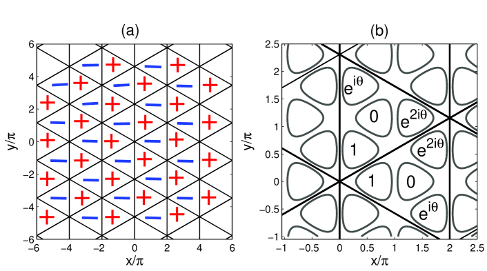
Figure 3: (Color online) Schematic depiction of the discrete vortex structure of the superfluid state $|\Psi_{+}\rangle$ (24). (a) The distribution of the vortices and anti-vortices in the elementary triangles of Fig. 2. (b) The distribution of the discrete vortex amplitude and phase between the wells (shown by contours) of the elementary triangles, with just two being shown, one containing the vortex and the other one – the anti-vortex. Here $\theta=\frac{2\pi}{3}$.

Due to the double degeneracy, the actual state of the system is defined, of course, by the nonlinear interaction part of the Hamiltonian $H_{R}$ (15). In our approximation, given by Eqs. (12) and (17), we have $U\langle a^{\dagger}a\rangle/J\ll 1$. Thus one can keep only the degenerate modes in the nonlinear term, which we denote as $\varphi_{+}\equiv\varphi_{{\bf 0},0,1}$ and $\varphi_{-}\equiv\varphi_{{\bf 0},0,2}$. Projecting on the degenerate subspace, we obtain

$$H^{(int)}=\frac{U}{(6\mathcal{N})^{2}}\left\{(\varphi^{\dagger}_{+})^{2}\varphi^{2}_{+}+(\varphi^{\dagger}_{-})^{2}\varphi^{2}_{-}+\varphi^{\dagger}_{+}\varphi_{+}\varphi^{\dagger}_{-}\varphi_{-}\right\}.$$ (23)

A simple analysis of Eq. (23) shows that the interaction energy is minimized when all atoms are in either one of the two Bloch modes $\varphi_{\pm}$. Each of the corresponding Bloch waves is a coherent superposition of the alternating discrete vortices and anti-vortices, each occupying just one of the elementary triangles, with the vortex centers being at the dissipative sites, as is easily seen from Eqs. (14) and (18), see Fig. 3. In the explicit form

$$|\Psi_{\pm}\rangle\propto\sum_{\bf q}\sum_{n=0}^{5}\{e^{\pm i\theta}|G_{{\bf q},n,1}\rangle+e^{\mp i\theta}|G_{{\bf q},n,2}\rangle+|G_{{\bf q},n,3}\rangle\},$$ (24)

where $\theta=2\pi/3$ and $|G_{{\bf q},n,l}\rangle$ is the ground state in the respective lattice well.

We note that though a macroscopic superposition of the two degenerate Bloch waves $|\Psi_{\pm}\rangle$ is permitted by the model, one must recall that the discarded terms of the full Hamiltonian and the nonlinear dissipation will eventually destroy the macroscopic coherence, thus one of the two superfluid states will be spontaneously selected. For instance, only the coherent superposition $\propto|\Psi_{+}\rangle-|\Psi_{-}\rangle$ with only three bosons in the system is the only null state of the nonlinear dissipation. Thus, the long-time state of BEC in the dissipative honeycomb optical lattice of Fig. 2 has the complex-valued order parameter with the vortex-like phase distribution.

IV Conclusion

In conclusion, we have introduced the notion of the dissipative optical lattice as the optical lattices with a sublattice of dissipative sites and have demonstrated its utility for engineering of the superfluid states of BEC with the complex-valued order parameter. The tight-binding approximation and the limit of a strong dissipation was used to allow for an analytical approach, since the numerical simulations would be difficult to carry out for the many-body open system on a lattice. We have found that the strong dissipation effectively changes the lattice space group, which results in a larger unit cell than that of the original optical lattice without the dissipation. Moreover, the base boson operators in the case of the dissipative lattice are linear superpositions of the local operators of the non-dissipative sites, what results in the ground state with a non-trivial complex-valued order parameter. For instance, in the dissipative honeycomb lattice the long-time ground state is a coherent superposition of the alternating discrete vortices and anti-vortices.

We have considered just two examples, the simple one-dimensional case and the honeycomb lattice, where we have chosen some particular distributions of the dissipative sites which allow one to obtain the long-term ground state in explicit analytical form. However, similar results are expected to hold quite generally for the optical lattices with a sublattice of dissipative sites. Moreover, similar behavior of BEC is expected in dissipative optical lattices in the continuous limit (as opposed to the tight-biding limit), which will be considered in a future publication.

- (1) L. Pitaevskii and S. Stringari, Bose-Einstein Condensation (Clarendon Press, Oxford, 2003)
- (2) D. Jaksch and P. Zoller, Ann. Phys. 315, 52 (2005).
- (3) O. Morsch and M. Oberthaler, Rev. Mod. Phys. 78, 179 (2006).
- (4) I. Bloch et al., Rev. Mod. Phys. 80, 885 (2008).
- (5) T. Gericke, C. Utfeld, N. Hommerstad and H. Ott, Las. Phys. Lett. 3, 415 (2006).
- (6) T. Gericke, P. Würtz, D. Reitz, T. Langen and H. Ott, Nat. Phys. 4, 949 (2008).
- (7) G. Wirth, M. Ölschläger and A. Hemmerich, Nat. Phys. 7, 147 (2011).
- (8) M. Ölschläger, G. Wirth and A. Hemmerich, Phys. Rev. Lett. 106, 015302 (2011).
- (9) P. Soltan-Panahi, D.-S. Lühmann, J. Struck, P. Windpassinger and K. Sengstock, Nat. Phys. 8, 71 (2012).
- (10) C. Wu, Mod. Phys. Lett. B 23, 1 (2009).
- (11) D. Mogilevtsev and V. S. Shchesnovich, Optt. Lett. 35, 3375 (2010).
- (12) V. S. Shchesnovich and D. Mogilevtsev, Phys. Rev. A 84, 013805 (2011).
- (13) F. Verstraete, M. M. Wolf and J. I. Cirac, Nat. Phys. 5, 633 (2009).
- (14) S. Diehl, A. Micheli, A. Kantian, B. Kraus, H. P. Büchler and P. Zoller, Nat. Phys. 4, 878 (2008).
- (15) A. Tomadin, S. Diehl and P. Zoller, Phys. Rev. A 83, 013611 (2011).
- (16) V. A. Brazhnyi, V. V. Konotop, V. M. Pérez-García, and H. Ott, Phys. Rev. Lett. 102, 144101 (2009).
- (17) D. Witthaut, F. Trimborn, and S. Wimberger, Phys. Rev. Lett. 101, 200402 (2008).
- (18) D. Witthaut, F. Trimborn, H. Hennig, G. Kordas, T. Geisel, and S. Wimberger, Phys. Rev. A 83, 063608 (2011).
- (19) B. Misra and E. C. G. Sudarshan, J. Math. Phys. 18, 756 (1977).
- (20) E. W. Streed, J. Mun, M. Boyd, G. K. Campbell, P. Medley, W. Ketterle, and D. E. Pritchard, Phys. Rev. Lett. 97, 260402 2006).
- (21) A.G. Kofman and G. Kurizki, Nature (London) 405, 546 (2000); Phys. Rev. Lett. 87, 270405 (2001).
- (22) P. Facchi and S. Pascazio, J. Phys. A: Math. Theor. 41, 493001 (2008).
- (23) V. S. Shchesnovich and V. V. Konotop, Phys. Rev. A 81, 053611 (2010).
- (24) H. Carmichael, An Open Systems Approach to Quantum Optics (Springer, Berlin, 1993); H. P. Breuer and F. Petruccione, The Theory of Open Quantum Systems (Oxford University Press, Oxford, 2002).
- (25) V. S. Shchesnovich, D. S. Mogilevtsev, Phys. Rev. A 82, 043621 (2010).
- (26) B. Wunsch, F. Guinea, and F. Sols, New J. Phys. 10, 103027 (2008).
- (27) Z. Chen and B. Wu, Phys. Rev. Lett. 107, 065301 (2011).
- (28) G. Grynberg, B. Lounis, P. Verkerk, J. Y. Courtois and C. Salomon, Phys. Rev. Lett. 70, 2249 (1993).
- (29) A. Klinger, S. Degenkolb, N. Gemelke, K.-A. Brickman Soderberg and C. Chin, Rev. Sci. Instr. 81, 013109 (2010).
- (30) V. S. Shchesnovich, A. S. Desyatnikov and Yuri S. Kivshar, Opt. Expr. 16, 14076 (2008).