State diagram and the phase transition of $p$-bosons in a square bi-partite optical lattice

Abstract

It is shown that, in a reasonable approximation, the quantum state of $p$-bosons in a bi-partite square two-dimensional optical lattice is governed by the nonlinear boson model describing tunneling of boson pairs between two orthogonal degenerate quasi momenta on the edge of the first Brillouin zone. The interplay between the lattice anisotropy and the atomic interactions leads to the second-order phase transition between the number-squeezed and coherent phase states of the $p$-bosons. In the isotropic case of the recent experiment, Nature Physicis 7, 147 (2011), the $p$-bosons are in the coherent phase state, where the relative global phase between the two quasi momenta is defined only up to mod($\pi$): $\phi=\pm\pi/2$. The quantum phase diagram of the nonlinear boson model is given.

Cold atoms and Bose-Einstein condensates in optical lattices provide a versatile tool for exploration of the quantum phenomena of condensed matter physics on one hand, and, on the other hand, a way for creation of novel types of order in cold atomic gases OPLAT . Two remarkable recent achievements in this direction are the experimentally demonstrated novel types of atomic superfluids in the $P$- Pboson and $F$-bands Fboson of the bi-partite square two-dimensional optical lattice. The bi-partite optical lattice having a checkerboard set of deep and shallow wells (i.e. made of double-wells), used in Refs. Pboson ; Fboson has a large coherence time in the higher bands, several orders of magnitude larger than the typical nearest-neighbor tunneling time CohTime . The order parameter of these superfluids is complex, in contrast to the conventional Bose-Einstein condensates having real order parameter in accord with Feynman’s no-node theorem for the ground state of a system of interacting bosons nonode ; Wu . The $p$-bosons, for instance, are confined to the second Bloch band for a sufficiently shallow lattice amplitude, $V_{0}\lesssim 2.2E_{R}$, where $E_{R}$ is the recoil energy CohTime ; InterRec . In Ref. Pboson $V_{0}\approx 1.55E_{R}$, however, a particular experimental technique was used which results in population of other Bloch bands. Nevertheless, the main results on the cross-dimensional coherence are obtained for the parameter values where the second band is by far the largest populated.

The purpose of this work is to show that, in the reasonable approximation, the quantum state of the $p$-bosons in the square bi-partite optical lattice is governed by the modified nonlinear boson model, which was already used before in the context of cold atoms tunneling between the high-symmetry points of the Brillouin zone SK ; SKPRL ; ParEff . However, there is an important difference: in the $p$-boson case there is a lattice asymmetry parameter which provides for the phase transition at the bottom of the energy spectrum, additionally to that at the top of the spectrum, studied before in Ref. SKPRL . The focus is on the quantum features of the $p$-boson superfluid, as different from Ref. CW where a mean-field Gross-Pitaevskii approach was employed and the region of the complex order parameter was found.

The nonlinear boson model derived below follows just from two basic conditions: the existence of two quasi degenerate energy states coupled by the boson pair exchange (tunneling) when the single-particle exchange is forbidden. Thus it applies to other contexts as well (see also Ref. ParEff ). For instance, it is equivalent to the nonlinear part of the so-called fundamental Hamiltonian (in the Wannier basis), describing the local two-flavor collisions in the first excited band of a two-dimensional single-well optical lattice CLM . Moreover, in the case of the optical lattice consisting of the one-dimensional double-wells ZPS the many-body Hamiltonian can be cast as a set of linearly-coupled nonlinear boson models. Taking this into account, we consider the quantum features of the derived nonlinear boson model in the most general setting and using its natural parameters, besides analyzing the experimental setting of Ref. Pboson .

Consider the bi-partite square two-dimensional optical lattice of Ref. Pboson , which can be cast as follows (after dropping an inessential constant term)

$$V = -V_{0}\exp\left(-\frac{z^{2}}{a^{2}_{z}}\right)\bigl{(}2v_{2,0}\cos(2kx)+2v_{0,2}\cos(2ky)$$ (1)

$$+2\mathrm{Re}\{v_{1,1}e^{ik(x+y)}+v_{-1,1}e^{ik(y-x)}\}\bigr{)},$$

where the experimental values of the parameters read $V_{0}=\overline{V}_{0}/4=1.55E_{R}$ in terms of the recoil energy $E_{R}=\frac{\hbar^{2}k^{2}}{2m}$, with $k=2\pi/\lambda$, $\lambda=1064\,$nm and $a_{z}=71\,\mu$m being the oscillator length of the transverse trap. The dimensionless Fourier amplitudes of the lattice are

$$v_{2,0}=\eta^{2}\epsilon\cos\alpha,\quad v_{1,1}=\eta\epsilon\left[e^{i\theta}+e^{-i\theta}\cos\alpha\right],$$

$$v_{0,2}=\epsilon,\quad v_{-1,1}=\eta\left[e^{i\theta}\cos\alpha+\epsilon^{2}e^{-i\theta}\right],$$ (2)

see Fig. 1. The experimental parameters are $\eta\approx 0.95$ and $\epsilon\approx 0.81$.

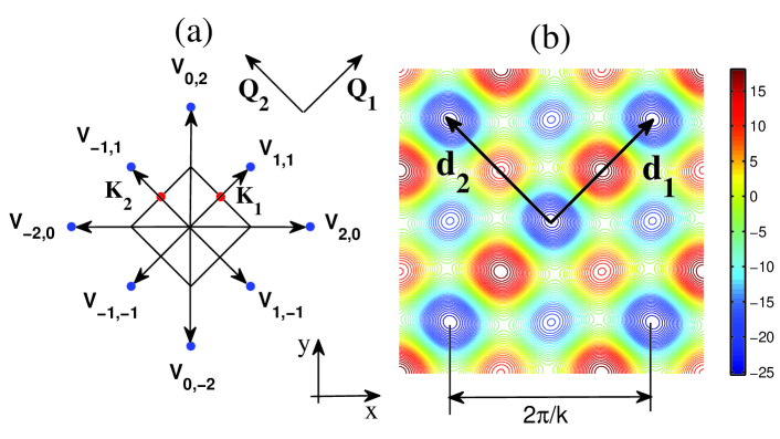
Figure 1: (Color online) Panel (a): The Fourier spectrum of the 2D lattice (1), where the Fourier amplitudes are shown by the (blue) dot markers and pointed by the reciprocal lattice vectors, the vectors ${\bf Q}_{1}=(k,k)$ and ${\bf Q}_{2}=(-k,k)$ give the reciprocal lattice periods, the points ${\bf K}_{1,2}$, shown by two (red) dot markers, are two nonequivalent minima of the second Bloch band. The square area is the first Brillouin zone. Panel (b): The bi-partite square lattice in the real space, the vectors ${\bf d}_{1}=(\frac{\pi}{k},\frac{\pi}{k})$ and ${\bf d}_{2}=(-\frac{\pi}{k},\frac{\pi}{k})$ form the basis of the lattice periods.

For $\alpha_{iso}=\arccos\epsilon\approx\pi/5$ and arbitrary values of the other parameters we have $v_{1,1}=v_{-1,1}$, hence, the lattice satisfies the symmetry $V(-x,y,z)=V(x,y,z)$. For $\alpha=\alpha_{iso}$ the band energies with the Bloch indices ${\bf K}_{1}=(\frac{k}{2},\frac{k}{2})$ and ${\bf K}_{2}=(-\frac{k}{2},\frac{k}{2})$ (see Fig. 1(a)) become equal, since the Bloch functions satisfy $\varphi_{{\bf K}_{1}}(-x,y,z)=\varphi_{{\bf K}_{2}}(x,y,z)$, due to the boundary conditions and symmetry of $V(x,y,z)$. Hence, the points ${\bf K}_{1,2}$ are the high-symmetry points of the symmetric lattice with (see also Ref. SK ).

As is found in Ref. CW the observed cross-dimensional coherence Pboson is the joint effect of the atomic interactions and the lattice potential. Indeed, let us estimate the interaction energy and its characteristic time scale in the $p$-boson experiment. The interaction energy can be estimated as $E_{int}\sim\frac{gN}{\Omega}$, where $g=\frac{4\pi\hbar^{2}a_{s}}{m}$ is the interaction coefficient proportional to the $s$-wave scattering length $a_{s}$, $N$ is the number of atoms and $\Omega$ is the effective volume of the condensate. Setting $\Omega=\sqrt{2\pi}a_{z}L^{2}\lambda^{2}$ (the coefficient is due to ground state of the transverse trap, see below), where $L$ is the number of the lattice sites along each of the two directions ${\bf d}_{1,2}$ in the plane ${\bf x}\equiv(x,y)$, we get $E_{int}\sim\frac{a_{s}N}{a_{z}L^{2}}E_{R}$. For ⁸⁷Rb and other experimental values of Ref. Pboson , with $N\sim 10^{5}$ and $L\sim 10$ (the estimated sample size of Ref. Pboson divided by the lattice cell size), we get $E_{int}/E_{R}\sim 0.1$. Moreover, the interaction time scale, defined as $t_{int}=\hbar/E_{int}$ is on the order of the typical experimental times, indeed, we have $t_{int}\sim\frac{ma_{z}L^{2}\lambda^{2}}{\hbar a_{s}N}\sim 10\,$ms (compare with Fig. 2 of Ref. Pboson ).

Taking into account the above estimate, one can assume that the atoms are confined to the second Bloch band of the lattice and expand the boson field operator over the band-limited Bloch basis. The Bloch waves are defined as $\varphi_{\bf k}({\bf x})=\frac{1}{L}e^{i{\bf k}{\bf x}}u_{{\bf k}}({\bf x})$, $u_{{\bf k}}({\bf x}+{\bf d}_{j})=u_{{\bf k}}({\bf x})$, $j=1,2$, where the periodic Bloch functions $u_{{\bf k}}({\bf x})$ are chosen to be normalized on the 2D lattice cell $\nu_{0}=|{\bf d}_{1}\times{\bf d}_{2}|$ of area $\lambda^{2}/2$, i.e.

$$\int\limits_{\nu_{0}}\mathrm{d}^{2}{\bf x}|u_{{\bf k}}({\bf x})|^{2}=1.$$

The band-limited expansion reads

$$\Psi({\bf x},z)=\sum_{{\bf k}\in B\!Z}b_{\bf k}\varphi_{{\bf k}}({\bf x})\Phi_{0}(z),$$ (3)

where the summation is over the Bloch indices inside the first Brillouin zone ${\bf k}\in\{\frac{\kappa_{1}}{L}{\bf Q}_{1}+\frac{\kappa_{2}}{L}{\bf Q}_{2};\;\kappa_{j}=-L/2,\ldots,L/2\}$ (see, Fig. 1(a)). Here $\Phi_{0}(z)$ is ground state $\Phi_{0}(z)\approx\pi^{-1/4}a_{z}^{-1/2}e^{-z^{2}/(2a_{z}^{2})}$ of the transverse trap. Inserting this expression into the standard Bose-Hubbard Hamiltonian for the lattice potential (1) and using the Poisson summation formula,

$$\sum_{\ell_{1},\ell_{2}=1}^{L}e^{i{\bf k}(\ell_{1}{\bf d}_{1}+\ell_{2}{\bf d}_{2})}=L^{2}\delta_{{\bf k},\bf{0}}\quad\mathrm{mod}({\bf Q}),$$

we obtain

$$H = \sum_{{\bf k}\in B\!Z}E({\bf k})b^{\dagger}{}_{\bf k}b_{\bf k}+\frac{g}{2\sqrt{2\pi}a_{z}}\int\mathrm{d}^{2}{\bf x}\left\{\left[\sum_{{\bf k}\in B\!Z}b^{\dagger}_{\bf k}\varphi^{*}_{{\bf k}}({\bf x})\right]^{2}\left[\sum_{{\bf k}\in B\!Z}b_{\bf k}\varphi_{{\bf k}}({\bf x})\right]^{2}\right\}$$ (4)

$$= \sum_{{\bf k}\in B\!Z}E({\bf k})b^{\dagger}{}_{\bf k}b_{\bf k}+\frac{g}{2\Omega}\sum_{\Delta_{{\bf k}}=\bf{0}}\chi({\bf k}_{1},{\bf k}_{2}|{\bf k}_{3},{\bf k}_{4})b^{\dagger}{}_{{\bf k}_{1}}b^{\dagger}{}_{{\bf k}_{2}}b_{{\bf k}_{3}}b_{{\bf k}_{4}},$$

where $E({\bf k})$ is the Bloch energy of the second band, $\Delta_{{\bf k}}\equiv{\bf k}_{1}+{\bf k}_{2}-{\bf k}_{3}-{\bf k}_{4}$, the condition $\Delta_{\bf k}=\bf{0}$ is understood mod(${\bf Q})$ and

$$\chi({\bf k}_{1},{\bf k}_{2}|{\bf k}_{3},{\bf k}_{4})=\nu_{0}\int\limits_{\nu_{0}}\mathrm{d}^{2}{\bf x}\,u^{*}_{{\bf k}_{1}}u^{*}_{{\bf k}_{2}}u_{{\bf k}_{3}}u_{{\bf k}_{4}}$$ (5)

is the dimensionless coefficient which depends solely on the lattice geometry.

Since the points ${\bf K}_{1,2}$, the energy minima of the second band, are lying on the edge of the Brillouin zone (Fig. 1(a)), the Bloch functions $\varphi_{{\bf K}_{1,2}}({\bf x})$ are real. Moreover $\nabla_{{\bf k}}E({\bf k})=0$ and, hence, $\nabla_{{\bf k}}\varphi_{{\bf K}_{1,2}}({\bf x})=0$. As the result, the expansion over ${\bf k}$ in Eq. (4) in some small neighborhoods about these points starts only with the second-order term $\propto({\bf k}-{\bf K}_{1,2})^{2}$ FootNote1 . On the other hand, one can verify that the experimental width of the Bragg peaks about the band minima ${\bf K}_{1,2}$ is too narrow to give a significant second-order correction, i.e. $({\bf k}-{\bf K}_{1,2})^{2}/k^{2}\sim 0.06$ (see, Fig. 3 of Ref. Pboson ). Therefore, we can discard the spectral width of the Bragg peaks and keep in Eq. (3) only the two-mode expansion of the boson field operator (a similar expansion over the two nonlinear modes was also used in Ref. CW )

$$\Psi({\bf x},z)\approx\left[b_{1}\varphi_{{\bf K}_{1}}({\bf x})+b_{2}\varphi_{{\bf K}_{2}}({\bf x})\right]\Phi_{0}(z).$$ (6)

It is important to note that, since the summation in the nonlinear term of Eq. (4) is conditioned by $\Delta_{\bf k}$=0 mod$({\bf Q}$), all terms with with either three ${\bf K}_{1}$ and one ${\bf K}_{2}$, or vice versa are zero (i.e. bosons tunnel between the minima by pairs SK ). Thus, only the following geometric parameters are nonzero:

$$\chi_{jj}=\nu_{0}\int\limits_{\nu_{0}}\mathrm{d}^{2}{\bf x}|u_{{\bf K}_{j}}({\bf x})|^{4},\quad j=1,2,$$

$$\chi_{12}=\nu_{0}\int\limits_{\nu_{0}}\mathrm{d}^{2}{\bf x}|u_{{\bf K}_{1}}({\bf x})u_{{\bf K}_{2}}({\bf x})|^{2}.$$ (7)

As a consequence, one obtains from Eq. (4) the two-mode Hamiltonian of the nonlinear boson model SK ; SKPRL ; ParEff except for the term proportional to the population imbalance due to the lattice asymmetry:

$$H = \frac{\mathcal{E}_{1}-\mathcal{E}_{2}}{2}(n_{1}-n_{2})+\frac{U}{2}\bigl{\{}n_{1}(n_{1}-1)+n_{2}(n_{2}-1)$$ (8)

$$+\Lambda(4n_{1}n_{2}+(b^{\dagger}{\!}_{1}b_{2})^{2}+(b^{\dagger}{\!}_{2}b_{1})^{2})\bigr{\}}.$$

We have denoted $n_{j}\equiv b^{\dagger}_{j}b_{j}$. The parameters of Hamiltonian (8) are as follows. The energies of the two symmetric points ${\bf K}_{1,2}$ read

$$\mathcal{E}_{1}=E_{1}+\frac{\chi_{11}}{2}\frac{gN}{\Omega},\quad\mathcal{E}_{2}=E_{2}+\frac{\chi_{22}}{2}\frac{gN}{\Omega},$$ (9)

where $E_{1,2}=E({\bf K}_{1,2})$ is the respective Bloch energy, $N=n_{1}+n_{2}$, $U$ is the average interaction parameter per particle,

$$U=\frac{g}{2\Omega}(\chi_{11}+\chi_{22}),$$ (10)

and $\Lambda$ is a pure geometric parameter defined as

$$\Lambda=2\chi_{12}/(\chi_{11}+\chi_{22}).$$ (11)

Note that at the symmetric point $\alpha=\alpha_{iso}$ we have $\sigma=0$, hence $\mathcal{E}_{1}=\mathcal{E}_{2}$. We have just two independent parameters $(\gamma,\Lambda)$, where $\gamma$ is defined as

$$\gamma=\frac{\mathcal{E}_{1}-\mathcal{E}_{2}}{UN}=\frac{E_{1}-E_{2}}{UN}+\sigma,\quad\sigma\equiv\frac{\chi_{11}-\chi_{22}}{\chi_{11}+\chi_{22}}.$$ (12)

Here we note that any 2D lattice which for some set of parameters possesses two non-equivalent points lying on the edge of the Brillouin zone and having equal Bloch energies can lead, under similar conditions, to the same model Hamiltonian (8).

The parameters $\Lambda$ and $\sigma$, $0\leq\Lambda\leq 1$ and $-1\leq\sigma\leq 1$, are independent of the interaction strength $g$ and are functions only of the lattice shape. For the experimental lattice (1) their dependence on $\alpha$ and $\theta$ can be determined by numerically solving the 2D eigenvalue problem for Bloch energies, the result is given in Fig. 2. Except for the semicircle shaped plateau, both parameters vary significantly with variation of the lattice potential. Specifically, for the experimental value $\theta=0.53\pi$ the parameters $\Lambda$, $\sigma$ and the Bloch energy difference are given in Fig. 3.

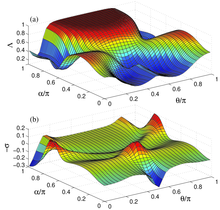
Figure 2: (Color online) The numerically computed lattice parameters $\Lambda$ (panel (a)) and $\sigma$ (panel(b)) for the experimental 2D lattice (1) of Ref. Pboson . Here $V_{0}=1.55E_{R}$, $\eta=0.95$, $\epsilon=0.81$. (The high accuracy Fourier pseudospectral method Pseudo was used.)

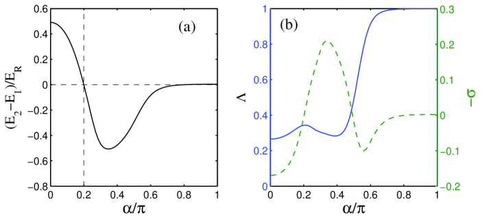
Figure 3: (Color online) The energy difference, (a), and the lattice parameters $\Lambda$ (the left $y$ axis, solid line) and $\sigma$ (the right $y$ axis, dashed line), (b). Here $\theta=0.53\pi$ and the other parameters are as in Fig. 2.

The interaction energy parameter $UN$ was already estimated above, i.e. $UN/E_{R}\sim{a_{s}N}/(a_{z}L^{2})\sim 0.1$ for the experimental values of Ref. Pboson , the bandgap is on the order of the lattice amplitude $V_{0}\sim E_{R}$, $\sigma\sim 0.2$, see Fig. 2(b), whereas the energy degeneracy is at most $\sim 0.4E_{R}$, see Fig. 3(a). We conclude that in the experiment of Ref. Pboson $\gamma$ can reach order $\sim 1$.

The ground state of the model Hamiltonian (8) for $\gamma\neq 0$ can be one of the two types of states: either the coherent phase state (with a definite relative phase between the two modes $b_{1,2}$, $\phi=\pm\pi/2$) or the atom number squeezed (Bogoliubov) state. These two types of the ground state are connected by the second-order quantum phase transition on the borderlines $\Lambda=1+|\gamma|$ in the plane $(\gamma,\Lambda)$ (see also Fig. 4 below). There are, in fact, exactly two phase transitions. One is at the bottom of the quantum energy spectrum and occurs for the asymmetry parameter $\gamma\neq 0$ (it corresponds to the relative phase $\pm\pi/2$, see below). The other one is at the top of the spectrum (and corresponds to the zero relative phase). For $\gamma=0$ the phase transition at the top of the spectrum was studied before SKPRL ; ParEff .

Consider first the number-squeezed states, which appear for the large population imbalance between the points ${\bf K}_{1,2}$ and have a squeezed variance of the population imbalance (see also Refs. SKPRL ; ParEff ). For instance, suppose that $n_{1}\gg n_{2}$ (i.e. $n_{1}\approx N$) and denote the respective class of states by $B_{1}$. Following Bogoluibov’s approach, one can replace $b_{1}\to\sqrt{N-n_{2}}e^{i\Phi}$, where $\Phi$ is an inessential random phase, and expand the Hamiltonian (8) in orders of $b_{2}$ and $b^{\dagger}_{2}$. Keeping the second-order terms only we get the local quadratic Hamiltonian in the form $H\approx\frac{UN^{2}}{2}\hat{H}_{1}$ with

$$\hat{H}_{1}=(1+\gamma)+2(2\Lambda-1+\gamma)\frac{n_{2}}{N}+\frac{\Lambda}{N}[(e^{i\Phi}b^{\dagger}_{2})^{2}+(e^{-i\Phi}b_{2})^{2}].$$ (13)

The Hamiltonian (13) is diagonalizable by the Bogoliubov transformation

$$b_{2}=e^{i\Phi}[\cosh\!\beta a-\sinh\!\beta a^{\dagger}],\;\tanh(2\beta)=\frac{\Lambda}{2\Lambda-1-\gamma}.$$ (14)

where $\beta$ is the squeezing parameter. We have

$$\hat{H}_{1}=1+\gamma+\frac{\Lambda}{N}\left[\frac{2}{\sinh(2\beta)}\left(a^{\dagger}a+\frac{1}{2}\right)-\coth(2\beta)\right].$$ (15)

For $n_{2}\gg n_{1}$ the number-squeezed states $B_{2}$ are described by similar quadratic Hamiltonian $\hat{H}_{2}$ obtained by replacing $b_{2}$ with $b_{1}$ in Eqs. (13)-(14) as well as inverting the sign at $\gamma$.

The existence diagram of the number-squeezed states $B_{1,2}$ is shown in Fig. 4(a), their existence is equivalent to existence of the Bogoliubov transformation (14). The states $B_{1,2}$ are thermodynamically stable for positive effective mass in Eq. (15), i.e. when $2\Lambda-1\mp\gamma>0$, which condition is satisfied only in the regions $\Lambda>1+\gamma$ and $\Lambda>1-\gamma$, respectively for $B_{1}$ and $B_{2}$. The thermodynamically stable $B_{1,2}$ states are shown in Fig. 4(d). Note that the number-squeezed states have undefined relative phase $\phi=\mathrm{arg}(\langle(b^{\dagger}_{1})^{2}b_{2}^{2}\rangle)/2$ (this is reflected also in arbitrariness of $\Phi$, see also the discussion of the quantum phase below).

Hamiltonian (8) also admits the phase states possessing definite values (i.e. with small variance) of the phase and the population imbalance. These states will be called coherent. The existence diagram of the coherent states can be found by approximating the Hamiltonian by a quantum oscillator problem in the Fock space SKPRL . For $N\gg 1$ the coherent states are essentially semiclassical in the sense of Ref. Braun . Thus, most of their properties can be studied by replacing the boson operators by scalar amplitudes: $b_{1}\to\sqrt{N/2(1+\zeta)}e^{-i\phi/2}$ and $b_{2}\to\sqrt{N/2(1-\zeta)}e^{i\phi/2}$ and considering the resulting classical model (save for the factor $\frac{UN^{2}}{2}$)

$$\mathcal{H}_{\mathrm{cl}}=\frac{1}{2}+\gamma\zeta+\frac{1}{2}\bigl{[}\zeta^{2}+\Lambda(1-\zeta^{2})(2+\cos(2\phi))\bigr{]}.$$ (16)

The stable stationary points of the classical Hamiltonian $\mathcal{H}_{\mathrm{cl}}$ correspond to the phase states of the quantum model. There are two stationary points: $(2\phi_{t}=0,\zeta_{t}=\frac{\gamma}{3\Lambda-1})$ and $(2\phi_{b}=\pi,\zeta_{b}=-\frac{\gamma}{1-\Lambda})$ and they correspond, respectively, the coherent phase states at the top ($C_{0}$) and at the bottom ($C_{\pi}$) of the quantum energy spectrum (this is clear from their energies).

The direct approach to study the coherent states is based on the discrete WKB in the Fock space, with the effective Planck constant $h=2/N$ SKPRL . One first factors out the classical phase $\phi_{b,t}$ and then expands the Hamiltonian (8) about the classical stationary point $\zeta_{b,t}$ (see also Ref. ST ). Representing the Fock-space “wave function” $\psi(\zeta)=\langle n,N-n|\psi\rangle$ (here $n\equiv n_{1}$) with $\zeta=2n/N-1$ as $\psi=e^{i\phi\zeta/h}\psi_{0}(\zeta)$ and defining the canonical with $\zeta$ momentum as $\hat{p}=-ih\partial_{\zeta}$ we get

$$\langle n,N-n|H|\psi\rangle=e^{i\phi\zeta/h}\frac{UN^{2}}{2}\hat{H}_{\phi}\psi_{0}(\zeta),$$ (17)

with a local Hamiltonian $\hat{H}_{\phi}$ of a quantum oscillator (the discarded terms start with $\sim(\zeta-\zeta_{b,t})^{3}$). The Hamiltonian about $\zeta_{b}$ (for the phase $2\phi_{b}=\pi$) reads

$$\hat{H}_{\phi_{b}}=\frac{1-\gamma^{2}-\Lambda^{2}}{2(1-\Lambda)}+\frac{1-\Lambda}{2}(\zeta-\zeta_{b})^{2}+\frac{\Lambda}{4}(1-\zeta_{b}^{2})\hat{p}^{2},$$ (18)

while that about the point $\zeta_{t}$ (for $2\phi_{t}=0$) can be obtained by replacing $\Lambda$ by $3\Lambda$ in the first two terms in Eq. (18) and inverting the sign at $\hat{p}^{2}$ due to the negative effective mass $M_{b,t}^{-1}=-\Lambda/2(1-\zeta_{b,t}^{2})\cos(2\phi_{b,t})$. The existence and stability analysis is straightforward from this point. First of all, the coherent states $C_{0}$, i.e. with the classical phase satisfying $2\phi_{t}=0$, are thermodynamically unstable due to the negative effective mass, while the states $C_{\pi}$ are thermodynamically stable where they exist. The existence diagram of the coherent states is given in Figs. 4(b) and (c). Numerical simulations confirm that the Gaussian width of the oscillator “wave-function” $\psi(\zeta)$ reasonably approximates the width of the coherent states in the Fock space.

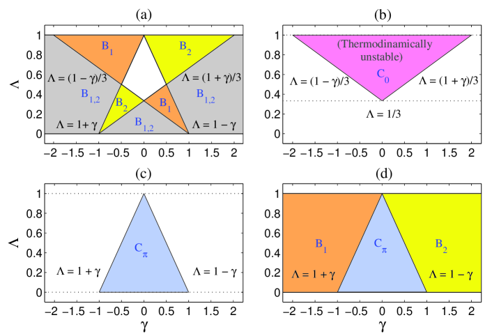
Figure 4: (Color online) (a) The existence diagram of the number-squeezed (Bogoliubov) states $B_{1,2}$ of Hamiltonian (8). (b) The coherent states of zero relative phase, corresponding to the top of the quantum energy spectrum ($C_{0}$). (c) The coherent states with the relative phase $\phi=\pm\pi/2$, corresponding to the bottom of the quantum energy spectrum ($C_{\pi}$). (d) The ground state diagram of the model Hamiltonian (8).

By considering the characteristic energies (up to $\sim 1/N$) in terms of $UN^{2}/2$ of all the above classes of states, i.e. $E(B_{1,2})=1\pm\gamma$, $E(C_{\pi})=\frac{1-\gamma^{2}-\Lambda^{2}}{2(1-\Lambda)}$ and $E(C_{0})=\frac{1-\gamma^{2}-9\Lambda^{2}}{2(1-3\Lambda)}$, one obtains the state diagram of the model (8), see Fig. 4(d). Depending on the values of $\gamma$ and $\Lambda$ the ground state is either the coherent state $C_{\pi}$ or one of the squeezed states, $B_{1}$ or $B_{2}$. The phase transition borderline is $\Lambda=1+|\gamma|$. Figs. 4(a) and (b) demonstrate that a similar phase transition occurs at the top of the energy spectrum on the border line given by $\Lambda=(1+|\gamma|)/3$. It was the subject of Refs. SKPRL ; ParEff .

Let us now consider the state diagram versus the experimental parameter $\alpha$. To compare the result also to the mean-field diagram of Ref. CW (see Fig. 5) one has to identify the same interaction parameter (the product of the $g$ and the density in Ref. CW ). The quantity $gN/\Omega$ can serve as an analog, though one has to remember that we have discarded the atoms of the condensate not represented by the Bragg peaks at the two points ${\bf K}_{1,2}$, thus the resulting approximate value of $gN/\Omega$ will be smaller than the actual value and the comparison can be only qualitative. The expressions for the borderlines $\Lambda=1\pm\gamma$ of the state diagram Fig. 4(d) can be rewritten using Eqs. (9), (10) and (12) as to give the interaction parameter $gN/\Omega$. We obtain:

$$g\frac{N}{\Omega}=\frac{E_{2}-E_{1}}{\chi_{11}-\chi_{12}},\quad\gamma\leq 0,$$ (19)

$$g\frac{N}{\Omega}=\frac{E_{1}-E_{2}}{\chi_{22}-\chi_{12}},\quad\gamma\geq 0.$$ (20)

The results are presented in Fig. 5, where the energy is given in the recoil energy units. Qualitatively we have similar diagram to that of Ref. CW , though the corresponding quantitative value of the interaction parameter $gN/\Omega$ is significantly smaller (though the density parameters are not identical, as mentioned above, the difference is still significant). We note, however, that the values of the interaction parameter in Fig. 5 do correspond to the estimated value $gN/\Omega\sim UN\sim 0.1E_{R}$ which accounts, for instance, for the Bragg peak formation times. This estimate was used to validate the expansion (6) over the Bloch modes, which was then used in the nonlinear part of the many-body boson Hamiltonian to produce the model Hamiltonian (8). For this very reason only the lower part of the figure around the critical $\alpha_{iso}$ belongs to the validity region of the approximation. Finally, an analog of the relative populations of the two modes is the semiclassical imbalance $\zeta_{b}$ (defined only for the coherent states). It can be cast as

$$\zeta_{b}=-\frac{\gamma}{1-\Lambda}=\frac{\chi_{22}-\chi_{11}+2(E_{2}-E_{1})\Omega/(gN)}{\chi_{11}+\chi_{22}-2\chi_{12}},$$ (21)

see Fig. 5(b).

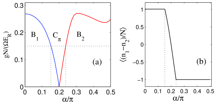
Figure 5: (Color online) (a) The phase diagram of the model Hamiltonian (8) in terms of the effective interaction parameter $g\frac{N}{\Omega}$ in units of the recoil energy vs. the angle $\alpha$. Here $\theta=0.53\pi$ and the rest of the parameters as in Fig. 2. (b) The typical average relative population imbalance between the two points ${\bf K}_{1,2}$, which correspond to the semiclassical $\zeta_{b}$ between two values of $\alpha$ (the dotted lines in (a) and (b)).

Finally, let us make some comments on the relative phase $\phi$. Why the phase $2\phi$ appears in the classical Hamiltonian $\mathcal{H}_{\mathrm{cl}}$ (16) is clear: the bosons tunnel by pairs, which is reflected in the splitting of the even and odd subspaces of the Fock space, with the respective basis states $|2s,N-2s\rangle$ and $|2s-1,N-2s+1\rangle$ SKPRL ; ParEff . Since the state of the system is always expanded over the states differing by an even number of bosons, it is impossible to define the phase $\phi$, but only the $2\phi$: $2\phi=\mathrm{arg}(\langle(b^{\dagger}_{1})^{2}b_{2}^{2}\rangle$). Hence $2\phi$ and not $\phi$ appears in the exponent factor in Eq. (17): $\exp\{i\phi\zeta/h\}=\exp\{2i\phi(n_{1}-n_{2})\}$. The splitting of the Fock space into two subspaces also leads to the double degeneracy of the coherent states (quasi-degeneracy to be precise: the terms of order $1/N$ are neglected), since the same approximate “wave-function” in the Fock space $\psi(\zeta)$ describes not one but two states, one of each subspace: $C_{2s}=\langle 2s,N-2s|\psi\rangle$ and $C_{2s-1}=\langle 2s-1,N-2s+1|\psi\rangle$ with the discrete sets $\zeta_{1}\in\{(2s-1)/N-1\}$ and $\zeta_{2}\in\{2s/N-1\}$.

The mean-field approach, in contrast, produces a definite relative phase, see Ref. CW , where two equivalent order parameters of the nonlinear Gross-Pitaevskii equation are possible for the description of the same experiment with the phase either $\pm\pi/2$, due to the broken superposition principle by the nonlinearity. However, the full many-body quantum Hamiltonian permits superposition of the eigenstates of the same energy. The resolution of this seemingly paradoxical situation is similar to the case of the random phase in the double-slit experiment with the Bose-Einstein condensate, see Ref. QPhase . Indeed, since the atoms are detected one by one coherently from both modes $b_{1,2}$, when the lattice is released, the atom detections probe the quantity $\langle b^{\dagger}_{1}b_{2}\rangle$ spontaneously projecting, as the detection process proceeds, on one of the two possible phases $\phi_{b}=\pm\pi/2$ of $C_{\pi}$.

In conclusion, we have shown that the experiment of Ref. Pboson is describable by the quantum model (8) and that there is the quantum phase transition of the second order between the atom number-squeezed states and the coherent phase states of the $p$-bosons. The results indicate that in the recent experiment Pboson a phase transition of the second order was observed, where the isotropic experimental state observed for the symmetric point $\alpha=\mathrm{arccos}\epsilon$ (and hence, for $\gamma=0$) must be the coherent $C_{\pi}$ state of the relative phase $2\phi=\pi$.

- (1) See, for instance, M. Lewenstein et al., Adv. Phys. 56, 243 (2007); I. Bloch et al., Rev. Mod. Phys. 80, 885 (2008).
- (2) G. Wirth, M. Ölschläger, and A. Hemmerich, Nat. Phys. 7, 147 (2011).
- (3) M. Ölschläger, G. Wirth, and A. Hemmerich, Phys. Rev. Lett. 106, 015302 (2011).
- (4) V. M. Stojanović, C. Wu, W. V. Liu and S. DasSarma, Phys. Rev. Lett. 101, 125301 (2008).
- (5) R. P. Feynman, Statistical Mechanics: A Set of Lectures (Addison-Wesley, Reading, MA, 1972).
- (6) C. Wu, Mod. Phys. Lett. B 23, 1 (2009).
- (7) J. Sebby-Strabley et al., Phys. Rev. A 73, 033605 (2006); Phys. Rev. Lett. 98, 200405 (2007); P. J. Lee et al., Phys. Rev. Lett. 99, 020402 (2007); M. Anderlini et al., Nature (London) 448, 452 (2007).
- (8) V. S. Shchesnovich and V. V. Konotop, Phys. Rev. A 75, 063628 (2007).
- (9) V. S. Shchesnovich and V. V. Konotop, Phys. Rev. Lett. 102, 055702 (2009).
- (10) V. S. Shchesnovich, Phys. Rev. A 80, 031601(R) (2009).
- (11) Z. Cai and C. Wu, cond-mat/11061121.
- (12) A. Collin, J. Larson and J.-P. Martikainen, Phys. Rev. A 81, 23605 (2010).
- (13) Q. Zhou, J. V. Porto and S. DasSarma, Phys. Rev. B 83, 195106 (2011).
- (14) The same conclusion follows also from Eq. (5), since leads to the form where is real and satisfies . Therefore, under the condition mod, the expansion of (5) also starts with the second order correction term in a small neighborhood about .
- (15) B. Fornberg, A Practical Guide to Pseudospectral Methods (Cambridge University Press, Cambridge, UK, 1996); L. N. Trefethen, Spectral Methods in Matlab (SIAM, Philadelphia, PA, 2000).
- (16) P. A. Braun, Rev. Mod. Phys. 65, 115 (1993).
- (17) V. S. Shchesnovich and M. Trippenbach, Phys. Rev. A 78, 023611 (2008).
- (18) J. Javanainen and S. M. Yoo, Phys. Rev. Lett. 76, 161 (1996); Y. Castin and J. Dalibard, Phys. Rev. A 55, 4330 (1997).