A Recursive Method to Calculate UV-divergent Parts at One-Loop Level in Dimensional Regularization

Abstract

A method is introduced to calculate the UV-divergent parts at one-loop level in dimensional regularization. The method is based on the recursion, and the basic integrals are just the scaleless integrals after the recursive reduction, which involve no other momentum scales except the loop momentum itself. The method can be easily implemented in any symbolic computer language, and an implementation in Mathematica is ready to use.

PROGRAM SUMMARY

• Title of program: $UVPart

• Programming language: Mathematica

• Available from: http://power.itp.ac.cn/~fengfeng/uvpart/

• Computer(s) for which the program has been designed: Any computer where the Mathematica is running.

• External routines/libraries used: FeynCalc, FeynArts

• Keywords: UV-Divergences, One-Loop Corrections, Dimensional Regularization

• CPC Library Classification: 11.1

• Nature of problem: To get the UV-divergent part of any one-loop expression.

• Method of solution: $UVPart is an Mathematica package where the recursive method has been implemented.

• Running time: In general it is below a second.

LONG WRITE-UP

I Introduction

One has to deal with an integration over the loop momentum at next-to-leading order, which results to ultraviolet (UV) and infrared (IR) divergencies. Dimensional regularization'tHooft:1972fi ; 'tHooft:1973us is needed in order to produce meaningful results. The general one-loop amplitude can be written as of a linear combination of known scalar integrals'tHooft:1978xw — boxes, triangles, bubbles and tadpoles — multiplied by coefficients that are rational functions of the external momenta and polarization vectors, plus a remainder which is also a rational function of the latter.

There are many automatic tools available to achieve the general one-loop amplitude, like FeynCalcMertig:1990an and FormCalchep-ph/9807565 , which are based on the traditional Passarino-VeltmanPassarino:1978jh ; Denner:1991kt ; Denner:2002ii ; Denner:2005nn reduction of Feynman graphs, which can be generated automatically(FeynArtsPrint-90-0144 (WURZBURG) ; hep-ph/0012260 or QGRAFNogueira:1991ex ). In order to produce numerical results, tensor coefficients functions are calculated using LoopToolshep-ph/9807565 . For a detailed review, please see Refs. hep-ph/9602280 ; arXiv:0903.4665 .

In the last few years, several groups have been working on the problem of constructing efficient and automatized methods for the computation of one-loop corrections for multi-particle processes. Many different interesting techniques have been proposed: these contain numerical and semi-numerical methodshep-ph/0402152 ; hep-ph/0508308 ; arXiv:0704.1835 ; arXiv:0708.2398 , as well as analytic approacheshep-ph/9409265 ; hep-ph/9403226 ; hep-th/0403047 ; hep-th/0406177 that make use of unitarity cuts to build NLO amplitudes by gluing on-shell tree amplitudeshep-ph/0602178 ; hep-th/0611091 . For a recent review of existing methods, see Refs. arXiv:0707.3342 ; arXiv:0704.2798 .

Generally, it will be much easier to calculate the UV-divergent parts of the one-loop amplitude than the one-loop amplitude itself, and there are little work on this specific area since one usually need not to calculate this part separately. However if what we are concerned is the renormalization, we need to calculate the UV-divergent parts only, and moreover there are also some cases in which we have to calculate the UV-divergence separately, for example, most packages like FirearXiv:0807.3243 and ReduzeStuderus:2009ye , which implement the integration by parts (IBP) relationsChetyrkin:1981qh , treat the scaleless integrals as zero, i.e.

$$\int d^{4}k\;(k^{2})^{n}=0$$ (1)

however it is well known for the logarithmically divergent scaleless integrals that

$$\frac{\left(2\pi\mu\right)^{4-D}}{i\pi^{2}}\int d^{4}k\;\frac{1}{(k^{2})^{2}}=\frac{1}{\varepsilon_{\rm UV}}-\frac{1}{\varepsilon_{\rm IR}}\;,$$ (2)

so Eq. (1) does not distinguish the UV- and IR-divergence. This will be fine if we consider the amplitude as a whole, since the UV-divergent parts will be canceled by the counter-terms, and the left divergence will only be IR-divergent. But there is no way to know the IR-divergence from a specific Feynman diagram, which is very important when one considers the factorization, where one tries to identity the source of IR- divergence and factorize them out.

A method that allows the extraction of the UV-divergent part of an arbitrary 1-loop tensor N-point coefficient was presented in Ref. Sulyok:2006xp . We want to introduce another simple method to calculate the UV-divergent part in the dimensional regularization. The method is based on the recursion, and basic integrals are just the scaleless integrals after the recursive reduction, which involve no other momentum scales except the loop momentum itself. Since the computation in this method just involves algebraic rational operations, so it can be easily implemented in any symbolic computer language.

The paper is organized as follows: We introduce the definitions and notations in Sec. II, then describe the calculations in Sec. III, and in Sec. IV we give an implementation with Mathematica, and use this method in a specific process $e^{+}e^{-}\to J/\psi+\eta_{c}$, and finally comes the summary.

II Definitions and Notations

The general expression associated with UV-divergent parts at one-loop reads

$$\mathcal{I}=\frac{\left(2\pi\mu\right)^{4-D}}{i\pi^{2}}\int d^{D}k\frac{\mathcal{Q}}{\mathcal{N}_{1}^{n_{1}}\mathcal{N}_{2}^{n_{2}}\cdots\mathcal{N}_{N}^{n_{N}}}$$ (3)

with the denominators

$$\mathcal{N}_{i}=\left(k+q_{i}\right)^{2}-m_{i}^{2}+i\epsilon,$$ (4)

where $i\epsilon$ denotes the infinitesimally small positive imaginary part, $\mu$ is the reorganization scale, $D$ is the non-integer dimension of space-time defined as $D=4-2\varepsilon$, $q_{i}$ are linear combination of external momenta $p_{i}$, and the numerator $\mathcal{Q}$ is the polynomial of $k^{2}$ and $k\cdot p_{i}$.

The following identity about the scaleless integrals is well known in the calculations with dimensional regularization:

$$\frac{\left(2\pi\mu\right)^{4-D}}{i\pi^{2}}\int d^{D}k\left(k^{2}\right)^{n}=\left\{\begin{array}[]{ll}0&(n\neq-2)\\ \frac{1}{\varepsilon_{\rm UV}}-\frac{1}{\varepsilon_{\rm IR}}&(n=-2)\end{array}\right.,$$ (5)

where only the logarithmically divergent scaleless integral contributes the UV-divergence.

According to Lorentz covariance and oddness of the scaleless integrals, we have

$$\frac{\left(2\pi\mu\right)^{4-D}}{i\pi^{2}}\int d^{D}k\;k^{\mu_{1}}k^{\mu_{2}}\cdots k^{\mu_{m}}\left(k^{2}\right)^{n}=\left\{\begin{array}[]{ll}0&(\mbox{m is odd})\\ \mathcal{C}_{m,n}\times g^{\{\mu_{1}\mu_{2}\cdots\mu_{m}\}}&(\mbox{m is even})\end{array}\right.,$$ (6)

i.e. when $m$ is odd, the scaleless tensor integrals are 0, and when $m$ is even, they are proportional to $g^{\{\mu_{1}\mu_{2}\cdots\mu_{m}\}}$ with coefficient $\mathcal{C}_{m,n}$, where we use the same notations as Refs. Sulyok:2006xp ; Denner:2005nn for $g^{\{\mu_{1}\mu_{2}\cdots\mu_{m}\}}$, which is the symmetrization of $g^{\mu_{1}\mu_{2}}g^{\mu_{3}\mu_{4}}\cdots g^{\mu_{m-1}\mu_{m}}$ with respect to the lorentz index $\mu_{1},\mu_{2},\cdots,\mu_{m}$, for example

$$g^{\{\mu_{1}\mu_{2}\}} = g^{\mu_{1}\mu_{2}},$$

$$g^{\{\mu_{1}\mu_{2}\mu_{3}\mu_{4}\}} = g^{\mu_{1}\mu_{2}}g^{\mu_{3}\mu_{4}}+g^{\mu_{1}\mu_{3}}g^{\mu_{2}\mu_{4}}+g^{\mu_{1}\mu_{4}}g^{\mu_{2}\mu_{3}}.$$ (7)

The coefficient $\mathcal{C}_{m,n}$ can be ready achieved by multiplying Eq. (6) with the $\displaystyle\frac{m}{2}$ metric tensors $g_{\mu_{1}\mu_{2}}g_{\mu_{3}\mu_{4}}\cdots g_{\mu_{m-1}\mu_{m}}$ and contracting the indexes,

$$\mathcal{C}_{m,n} = \frac{1}{D(D+2)\cdots(D+m-2)}\frac{\left(2\pi\mu\right)^{4-D}}{i\pi^{2}}\int d^{D}k\left(k^{2}\right)^{n+\frac{m}{2}}$$ (10)

$$= \left\{\begin{array}[]{ll}0&(n+\frac{m}{2}\neq-2)\\ \frac{1}{D(D+2)\cdots(D+m-2)}\left[\frac{1}{\varepsilon_{\rm UV}}-\frac{1}{\varepsilon_{\rm IR}}\right]&(n+\frac{m}{2}=-2)\end{array}\right.,$$

where we have used

$$g_{\mu_{1}\mu_{2}}g_{\mu_{3}\mu_{4}}\cdots g_{\mu_{m-1}\mu_{m}}g^{\{\mu_{1}\mu_{2}\cdots\mu_{m}\}}=D(D+2)\cdots(D+m-2)\;,$$ (11)

where $m$ is even, and more relations can be found in Ref. Sulyok:2006xp .

III Description of the Calculations

We define a function Power to get the asymptotic scaling of the polynomial of $k^{2}$ and $k\cdot p_{i}$ in the ultraviolet region, for example:

$$\texttt{Power}[k^{2}]=2,\;\texttt{Power}[k\cdot p_{i}]=1,\;\texttt{Power}[m^{2}]=0,\;\texttt{Power}[k^{2}+k\cdot p_{i}-m^{2}]=2$$ (12)

and we can extend this function to rational expression of $k^{2}$ and $k\cdot p_{i}$.

$$\texttt{Power}\left[\frac{\mathcal{N}}{\mathcal{D}}\right]\equiv\texttt{Power}[\mathcal{N}]-\texttt{Power}[\mathcal{D}],$$ (13)

where $\mathcal{N}$ and $\mathcal{D}$ are some polynomials of $k^{2}$ and $k\cdot p_{i}$, for example

$$\texttt{Power}\left[\frac{k\cdot p_{1}}{\left(k^{2}-m_{0}^{2}\right)\left((k+q_{1})^{2}-m_{1}^{2}\right)^{2}}\right]=-5.$$ (14)

So if Power of the integrand in $\mathcal{I}$ is less than -4, then there will be no UV-divergent part in $\mathcal{I}$. i.e.

$$\mathcal{I}_{\rm UV}=0,\quad(\texttt{Power}[\mathcal{Q}]-\sum_{i}^{N}2n_{i}<-4).$$ (15)

For example

$$\left[\frac{\left(2\pi\mu\right)^{4-D}}{i\pi^{2}}\int d^{D}k\frac{k\cdot p_{1}}{\left(k^{2}-m_{0}^{2}\right)\left((k+p_{1})^{2}-m_{1}^{2}\right)^{2}}\right]_{\rm UV}=0.$$ (16)

Now we are going to describe the calculations of UV-divergent parts of $\mathcal{I}$. For general integrand of $\mathcal{I}$, we can write

$$\frac{\mathcal{Q}}{\mathcal{N}_{1}^{n_{1}}\mathcal{N}_{2}^{n_{2}}\cdots\mathcal{N}_{N}^{n_{N}}} = \frac{\mathcal{N}_{1}-\left(\mathcal{N}_{1}-k^{2}\right)}{k^{2}}\frac{\mathcal{Q}}{\mathcal{N}_{1}^{n_{1}}\mathcal{N}_{2}^{n_{2}}\cdots\mathcal{N}_{N}^{n_{N}}}$$ (17)

$$= \frac{\mathcal{Q}}{k^{2}\mathcal{N}_{1}^{n_{1}-1}\mathcal{N}_{2}^{n_{2}}\cdots\mathcal{N}_{N}^{n_{N}}}-\frac{\mathcal{Q}^{\prime}}{k^{2}\mathcal{N}_{1}^{n_{1}}\mathcal{N}_{2}^{n_{2}}\cdots\mathcal{N}_{N}^{n_{N}}}$$

with $\mathcal{Q}^{\prime}=\mathcal{Q}\,\left(\mathcal{N}_{1}-k^{2}\right)$, and it is clear that

$$\texttt{Power}\left[\frac{\mathcal{Q}^{\prime}}{k^{2}\mathcal{N}_{1}^{n_{1}}\mathcal{N}_{2}^{n_{2}}\cdots\mathcal{N}_{N}^{n_{N}}}\right]\leq\texttt{Power}\left[\frac{\mathcal{Q}}{\mathcal{N}_{1}^{n_{1}}\mathcal{N}_{2}^{n_{2}}\cdots\mathcal{N}_{N}^{n_{N}}}\right]-1,$$ (18)

i.e. either the power of propagators: $n_{i}$ or the Power of the integrand decreases by at least 1, if we apply this replacement once again in the last result, we have

$$\frac{\mathcal{Q}}{\mathcal{N}_{1}^{n_{1}}\mathcal{N}_{2}^{n_{2}}\cdots\mathcal{N}_{N}^{n_{N}}} = \left[\frac{\mathcal{Q}}{\left(k^{2}\right)^{2}\mathcal{N}_{1}^{n_{1}-2}\mathcal{N}_{2}^{n_{2}}\cdots\mathcal{N}_{N}^{n_{N}}}-\frac{\mathcal{Q}^{\prime}}{\left(k^{2}\right)^{2}\mathcal{N}_{1}^{n_{1}-1}\mathcal{N}_{2}^{n_{2}}\cdots\mathcal{N}_{N}^{n_{N}}}\right]$$ (19)

$$-\left[\frac{\mathcal{Q}^{\prime}}{\left(k^{2}\right)^{2}\mathcal{N}_{1}^{n_{1}-1}\mathcal{N}_{2}^{n_{2}}\cdots\mathcal{N}_{N}^{n_{N}}}-\frac{\mathcal{Q}^{\prime\prime}}{\left(k^{2}\right)^{2}\mathcal{N}_{1}^{n_{1}}\mathcal{N}_{2}^{n_{2}}\cdots\mathcal{N}_{N}^{n_{N}}}\right],$$

with $\mathcal{Q}^{\prime\prime}=\mathcal{Q}^{\prime}\,\left(\mathcal{N}_{1}-k^{2}\right)$, and we can see the power of propagators: $n_{i}$ or the Power of the integrand decreases further by at least 1.

So we can apply this replacement again and again until one of the following cases happens:

• All the power of $\mathcal{N}_{i}$, becomes zero, i.e. only one type of propagator: $k^{2}$ is left.

• The corresponding $\mathcal{I}_{\rm UV}=0$, i.e.

  $$\texttt{Power}\left[\frac{\mathcal{Q}}{\mathcal{N}_{1}^{n_{1}}\mathcal{N}_{2}^{n_{2}}\cdots\mathcal{N}_{N}^{n_{N}}}\right]=\left(\texttt{Power}[\mathcal{Q}]-\sum_{i}^{N}2n_{i}\right)<-4.$$

So after the recursive reduction, only one type of integration will be left:

$$\mathcal{I}=\frac{\left(2\pi\mu\right)^{4-D}}{i\pi^{2}}\int d^{D}k\frac{\mathcal{Q}}{\left(k^{2}\right)^{n}}\;,$$ (20)

and it is ready to read the result according to Eqs. (5) and (6).

We can take the following 3-point tensor integral as an example:

$$\frac{(k\cdot p_{1})^{3}}{k^{2}\left[\left(k+q_{1}\right)^{2}-m_{1}^{2}\right]\left[\left(k+q_{2}\right)^{2}-m_{2}^{2}\right]}$$ (21)

$$\to \frac{(k\cdot p_{1})^{3}}{\left(k^{2}\right)^{2}\left[\left(k+q_{2}\right)^{2}-m_{2}^{2}\right]}-\frac{(k\cdot p_{1})^{3}\left(2k\cdot q_{1}+{\color[rgb]{0,0,0}\framebox{$\displaystyle\color[rgb]{0,0,0}q_{1}^{2}-m_{1}^{2}$}}\right)}{\left(k^{2}\right)^{2}\left[\left(k+q_{1}\right)^{2}-m_{1}^{2}\right]\left[\left(k+q_{2}\right)^{2}-m_{2}^{2}\right]}$$

$$\to \left[\frac{(k\cdot p_{1})^{3}}{\left(k^{2}\right)^{3}}-\frac{(k\cdot p_{1})^{3}\left(2k\cdot q_{2}+{\color[rgb]{0,0,0}\framebox{$\displaystyle\color[rgb]{0,0,0}q_{2}^{2}-m_{2}^{2}$}}\right)}{\left(k^{2}\right)^{3}\left[\left(k+q_{2}\right)^{2}-m_{2}^{2}\right]}\right]$$

$$-\left[\frac{(k\cdot p_{1})^{3}\left(2k\cdot q_{1}\right)}{\left(k^{2}\right)^{3}\left[\left(k+q_{2}\right)^{2}-m_{2}^{2}\right]}-{\color[rgb]{0,0,0}\framebox{$\displaystyle\color[rgb]{0,0,0}\frac{(k\cdot p_{1})^{3}\left(2k\cdot q_{1}\right)\left(2k\cdot q_{1}+q_{1}^{2}-m_{1}^{2}\right)}{\left(k^{2}\right)^{3}\left[\left(k+q_{1}\right)^{2}-m_{1}^{2}\right]\left[\left(k+q_{2}\right)^{2}-m_{2}^{2}\right]}$}}\right]$$

$$\to \frac{(k\cdot p_{1})^{3}}{\left(k^{2}\right)^{3}}-\frac{(k\cdot p_{1})^{3}\left(2k\cdot q_{2}\right)}{\left(k^{2}\right)^{4}}-{\color[rgb]{0,0,0}\framebox{$\displaystyle\color[rgb]{0,0,0}\frac{(k\cdot p_{1})^{3}\left(2k\cdot q_{2}\right)\left(2k\cdot q_{2}-m_{2}^{2}\right)}{\left(k^{2}\right)^{3}\left[\left(k+q_{2}\right)^{2}-m_{2}^{2}\right]}$}}$$

$$-\frac{(k\cdot p_{1})^{3}\left(2k\cdot q_{1}\right)}{\left(k^{2}\right)^{4}}-{\color[rgb]{0,0,0}\framebox{$\displaystyle\color[rgb]{0,0,0}\frac{(k\cdot p_{1})^{3}\left(2k\cdot q_{1}\right)\left(2k\cdot q_{2}-m_{2}^{2}\right)}{\left(k^{2}\right)^{3}\left[\left(k+q_{2}\right)^{2}-m_{2}^{2}\right]}$}}$$

$$\to \frac{(k\cdot p_{1})^{3}}{\left(k^{2}\right)^{3}}-\frac{(k\cdot p_{1})^{3}\left(2k\cdot q_{2}\right)}{\left(k^{2}\right)^{4}}-\frac{(k\cdot p_{1})^{3}\left(2k\cdot q_{1}\right)}{\left(k^{2}\right)^{4}}\;,$$

where each step $\displaystyle\to$ means we take a replacement, and all the expressions framed with box have been dropped during the recursive expansion since the Power is less than ${\tt-4}$ and will not contribute UV-divergent part.

Now it is ready to get the UV-divergent parts from the last line in Eq. (21), using Eqs. (5) and (6)

$$\left[\frac{\left(2\pi\mu\right)^{4-D}}{i\pi^{2}}\!\!\!\int d^{D}k\frac{(k\cdot p_{1})^{3}}{k^{2}\left[\left(k+q_{1}\right)^{2}-m_{1}^{2}\right]\left[\left(k+q_{2}\right)^{2}-m_{2}^{2}\right]}\right]_{\rm UV}\!\!\!\!=-\frac{p_{1}^{2}\left(p_{1}\cdot q_{1}+p_{1}\cdot q_{2}\right)}{4}\frac{1}{\varepsilon_{\rm UV}}$$ (22)

and we can check that it agrees with Refs. Sulyok:2006xp ; Denner:2005nn .

The important feature of this method is that, there is only one preliminary integral, i.e. Eq. (6), which involves no other scales like external momenta $p_{i}$ or mass $m_{i}$.

Another advantage is that it can be easily implemented in any symbolic computer language, like Mathematica, Reduce, Form, etc. I will give an explicit implementation with Mathematica in the next section.

IV Implementation With Mathematica

IV.1 Typical Examples

An implementation in Mathematica is already available, note that the FeynCalc package has been used to deal with the ScalarProduct, but it not required for the implementation.

The UV-divergent parts can be retrieved with the function: $UVPart, which is defined as:

$$\mbox{\frenchspacing$UVPart[exp,\ k]}:=\left[\frac{\left(2\pi\mu\right)^{4-D}}{i\pi^{2}}\int d^{D}\texttt{k}\;\texttt{exp}\right]_{\rm UV}$$ (23)

where exp can be any expression at one-loop level, while k is the loop momentum.

We can give some simple examples:

den=SPD[k] (SPD[k+q1]-m1^2) (SPD[k+q2]-m2^2)//FCI//ScalarProductExpand;
num=SPD[k, p1]^3//FCI;
$UVPart[num/den, k]//Simplify

The output of the code above reads:

$$\texttt{Out[ ]}:=-\frac{6\text{p1}^{2}(\text{p1}\cdot\text{q1}+\text{p1}\cdot\text{q2})}{D(D+2)\omega}\;,$$ (24)

where $\omega$ is just $\varepsilon_{\rm UV}$ which we have used to represent the UV divergence in the Mathematic code, Eq. (24) gives the same result as Eq. (22) after setting the dimension $D$ to 4.

den = (SPD[k]-m0^2) (SPD[k]-m1^2)^2 (SPD[k]-m2^2)//FCI//ScalarProductExpand;
num = SPD[k,p]^8//FCI;
$UVPart[num/den,k]

The output reads:

$$\texttt{Out[ ]}:=\frac{105\left(\text{m0}^{4}+\left(2\text{m1}^{2}+\text{m2}^{2}\right)\text{m0}^{2}+3\text{m1}^{4}+\text{m2}^{4}+2\text{m1}^{2}\text{m2}^{2}\right)(p^{2})^{4}}{D\left(D^{3}+12D^{2}+44D+48\right)\omega}\;,$$ (25)

setting $D$ to 4 we get

$$\left[\frac{\left(2\pi\mu\right)^{4-D}}{i\pi^{2}}\int d^{D}k\frac{(k\cdot p)^{8}}{\left(k^{2}-m_{0}^{2}\right)\left(k^{2}-m_{1}^{2}\right)^{2}\left(k^{2}-m_{2}^{2}\right)}\right]_{\rm UV}$$ (26)

$$= -\frac{7(p^{2})^{4}\left(m_{0}^{4}+m_{2}^{4}+3m_{1}^{4}+2m_{0}^{2}m_{1}^{2}+m_{0}^{2}m_{2}^{2}+2m_{1}^{2}m_{2}^{2}\right)}{128}\frac{1}{\varepsilon_{\rm UV}}\;.$$

IV.2 UV-Divergences in $e^{+}e^{-}\to J/\psi+\eta_{c}$ at One-Loop Level

We will apply the method to a specific process $e^{+}e^{-}\to J/\psi+\eta_{c}$, where we use the FeynArts to generate Feynman diagrams, and FeynCalc to handle the DiracTrace. We will take a triangle Feynman diagram in Fig. 1 as a concrete example in this section.

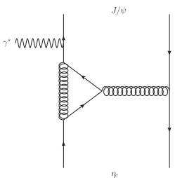
Figure 1: An triangle feynman diagram in $e^{+}e^{-}\to\gamma^{*}\to J/\psi+\eta_{c}$

First we use the FeynArts to generate the amplitude for the diagram, then make the following replacement with the help of spinor projectors hep-ph/0211085 :

$$v(\bar{p}_{3})\bar{u}(p_{3}) \to \frac{1}{4\sqrt{2}E_{3}(E_{3}+m_{c})}(\bar{p}\!\!\!/_{3}-m_{c})\epsilon_{S}^{*}(P\!\!\!\!/_{3}+2E_{3})(p\!\!\!/_{3}+m_{c})\otimes\frac{\bf 1}{\sqrt{N_{c}}}$$

$$v(\bar{p}_{4})\bar{u}(p_{4}) \to \frac{1}{4\sqrt{2}E_{2}(E_{4}+m_{c})}(\bar{p}\!\!\!/_{4}-m_{c})\gamma_{5}(P\!\!\!\!/_{4}+2E_{4})(p\!\!\!/_{4}+m_{c})\otimes\frac{\bf 1}{\sqrt{N_{c}}}$$ (27)

where the subscripts 3 and 4 are used to label $J/\psi$ and $\eta_{c}$ respectively.

After performing the DiracTrace on the fermion chains, we get the amplitude for this diagram as follows:

$${\rm Amp} = \frac{iC_{F}eg_{s}^{4}\epsilon^{\mu\epsilon_{S}^{*}p_{3}p_{4}}}{6\sqrt{N_{c}}m_{c}^{5}(s-4)s^{2}k^{2}\left(k^{2}+k\cdot p_{4}\right)\left(2sm_{c}^{2}+k^{2}+k\cdot p_{3}+2k\cdot p_{4}\right)}$$ (28)

$$\times\Big{(}\!\!-\!\!2Ds^{2}m_{c}^{4}+12s^{2}m_{c}^{4}+8Dsm_{c}^{4}-56sm_{c}^{4}+32m_{c}^{4}+8Dk^{2}m_{c}^{2}$$

$$-2Dsk^{2}m_{c}^{2}+4sk^{2}m_{c}^{2}-16k^{2}m_{c}^{2}+4Dk\cdot p_{3}m_{c}^{2}+D^{2}sk\cdot p_{3}m_{c}^{2}$$

$$-12Dsk\cdot p_{3}m_{c}^{2}+36sk\cdot p_{3}m_{c}^{2}-16k\cdot p_{3}m_{c}^{2}+4Dk\cdot p_{4}m_{c}^{2}$$

$$-D^{2}sk\cdot p_{4}m_{c}^{2}+10Dsk\cdot p_{4}m_{c}^{2}-32sk\cdot p_{4}m_{c}^{2}-2Dk\cdot p_{4}^{2}$$

$$+4k\cdot p_{4}^{2}+2Dk\cdot p_{3}k\cdot p_{4}-4k\cdot p_{3}k\cdot p_{4}\Big{)}\;,$$

where $p_{3}$ and $p_{4}$ are the momenta of $J/\psi$ and $\eta_{c}$ respectively, and $s=(p_{3}+p_{4})^{2}/(4m_{c}^{2})$, $m_{c}$ is the quark mass, and $k$ is the loop momentum, and to get the UV-divergent part of the amplitude, we just use

        $UVPart[Amp,k]

The output reads:

$$\texttt{Out[ ]}:=-\frac{iC_{F}(D-2)^{2}eg_{s}^{4}\epsilon^{\gamma\psi\text{p3}\text{p4}}}{3\sqrt{N_{c}}D\text{mc}^{3}s^{2}\omega}$$ (29)

where the Lorentz index $\gamma$ refers to $\mu$, and $\psi$ to $\epsilon_{S}^{*}$ in Eq. (28). After setting $D$ to 4, we get

$$\left[\frac{\left(2\pi\mu\right)^{4-D}}{i\pi^{2}}\int d^{D}k\;{\rm Amp}\right]_{\rm UV}=-\frac{iC_{F}eg_{s}^{4}\epsilon^{\mu\epsilon^{*}p_{3}p_{4}}}{3\sqrt{N_{c}}m_{c}^{3}s^{2}}\frac{1}{\varepsilon_{\rm UV}}$$ (30)

We can apply this method to each diagram to get the corresponding UV-divergent part of the amplitude, and to check the validity of the our result. We have compared the UV-divergent part produced with our code with Ref. Gong:2007db diagram by diagram, and the both agree with each other for all diagrams.

V Summary

A pretty simple method is introduced to calculate the UV-divergent parts at one-loop level with dimensional regularization. It is found that there is only one preliminary integral which involves no other scale like external momenta $p_{i}$ or mass $m_{i}$ after the recursive reduction. The method can be easily implemented in any symbolic computer language, An explicit implementation with Mathematica is also present.

References

• (1) G. ’t Hooft and M. J. G. Veltman, Regularization And Renormalization Of Gauge Fields, Nucl. Phys.  B 44 (1972) 189.
• (2) G. ’t Hooft, An algorithm for the poles at dimension four in the dimensional regularization procedure, Nucl. Phys.  B 62 (1973) 444.
• (3) G. ’t Hooft and M. J. G. Veltman, Scalar One Loop Integrals, Nucl. Phys.  B 153, 365 (1979).
• (4) R. Mertig, M. Bohm and A. Denner, FEYNCALC: Computer algebraic calculation of Feynman amplitudes, Comput. Phys. Commun.  64 (1991) 345.
• (5) T. Hahn and M. Perez-Victoria, Automatized one loop calculations in four-dimensions and D-dimensions, Comput. Phys. Commun.  118, 153 (1999) [hep-ph/9807565].
• (6) G. Passarino and M. J. G. Veltman, One Loop Corrections For $e^{+}e^{-}$ Annihilation Into $\mu^{+}\mu^{-}$ In The Weinberg Model, Nucl. Phys.  B 160 (1979) 151.
• (7) A. Denner, Techniques for calculation of electroweak radiative corrections at the one loop level and results for W physics at LEP-200, Fortsch. Phys.  41 (1993) 307 [arXiv:0709.1075 [hep-ph]].
• (8) A. Denner and S. Dittmaier, Reduction of one-loop tensor 5-point integrals, Nucl. Phys.  B 658 (2003) 175 [arXiv:hep-ph/0212259].
• (9) A. Denner and S. Dittmaier, Reduction schemes for one-loop tensor integrals, Nucl. Phys.  B 734 (2006) 62 [arXiv:hep-ph/0509141].
• (10) J. Kublbeck, M. Bohm and A. Denner, FeynArts: Computer Algebraic Generation Of Feynman Graphs And Amplitudes, Comput. Phys. Commun.  60, 165 (1990).
• (11) T. Hahn, Generating Feynman diagrams and amplitudes with FeynArts 3, Comput. Phys. Commun.  140, 418 (2001) [hep-ph/0012260].
• (12) P. Nogueira, Automatic Feynman graph generation, J. Comput. Phys.  105 (1993) 279.
• (13) Z. Bern, L. J. Dixon and D. A. Kosower, Progress in one loop QCD computations, Ann. Rev. Nucl. Part. Sci.  46, 109 (1996) [hep-ph/9602280].
• (14) A. van Hameren, C. G. Papadopoulos and R. Pittau, Automated one-loop calculations: A Proof of concept, JHEP 0909, 106 (2009) [arXiv:0903.4665 [hep-ph]].
• (15) W. T. Giele and E. W. N. Glover, A Calculational formalism for one loop integrals, JHEP 0404, 029 (2004) [hep-ph/0402152].
• (16) R. K. Ellis, W. T. Giele and G. Zanderighi, Semi-numerical evaluation of one-loop corrections, Phys. Rev. D 73, 014027 (2006) [hep-ph/0508308].
• (17) D. Forde, Direct extraction of one-loop integral coefficients, Phys. Rev. D 75, 125019 (2007) [arXiv:0704.1835 [hep-ph]].
• (18) R. K. Ellis, W. T. Giele and Z. Kunszt, A Numerical Unitarity Formalism for Evaluating One-Loop Amplitudes, JHEP 0803, 003 (2008) [arXiv:0708.2398 [hep-ph]].
• (19) Z. Bern, L. J. Dixon, D. C. Dunbar and D. A. Kosower, Fusing gauge theory tree amplitudes into loop amplitudes, Nucl. Phys. B 435, 59 (1995) [hep-ph/9409265].
• (20) Z. Bern, L. J. Dixon, D. C. Dunbar and D. A. Kosower, One loop n-point gauge theory amplitudes, unitarity and collinear limits, Nucl. Phys. B 425, 217 (1994) [hep-ph/9403226].
• (21) F. Cachazo, P. Svrcek and E. Witten, MHV vertices and tree amplitudes in gauge theory, JHEP 0409, 006 (2004) [hep-th/0403047].
• (22) F. Cachazo, P. Svrcek and E. Witten, Twistor space structure of one-loop amplitudes in gauge theory, JHEP 0410, 074 (2004) [hep-th/0406177].
• (23) R. Britto, B. Feng and P. Mastrolia, The Cut-constructible part of QCD amplitudes, Phys. Rev. D 73, 105004 (2006) [hep-ph/0602178].
• (24) P. Mastrolia, On Triple-cut of scattering amplitudes, Phys. Lett. B 644, 272 (2007) [hep-th/0611091].
• (25) S. Weinzierl, Automated calculations for multi-leg processes, PoSACAT , 005 (2007) [arXiv:0707.3342 [hep-ph]].
• (26) Z. Bern, L. J. Dixon and D. A. Kosower, On-Shell Methods in Perturbative QCD, Annals Phys.  322, 1587 (2007) [arXiv:0704.2798 [hep-ph]].
• (27) A. V. Smirnov, Algorithm FIRE – Feynman Integral REduction, JHEP 0810, 107 (2008) [arXiv:0807.3243 [hep-ph]].
• (28) C. Studerus, Reduze - Feynman Integral Reduction in C++, Comput. Phys. Commun.  181, 1293 (2010) [arXiv:0912.2546 [physics.comp-ph]].
• (29) K. G. Chetyrkin and F. V. Tkachov, Integration By Parts: The Algorithm To Calculate Beta Functions In 4 Loops, Nucl. Phys.  B 192 (1981) 159.
• (30) G. Sulyok, UV-divergent parts of the Passarino-Veltmann functions in dimensional regularisation, [hep-ph/0609282].
• (31) E. Braaten and J. Lee, Exclusive double charmonium production from $e^{+}e^{-}$ annihilation into a virtual photon, Phys. Rev. D 67, 054007 (2003) [Erratum-ibid. D 72, 099901 (2005)] [hep-ph/0211085].
• (32) B. Gong and J. X. Wang, QCD corrections to $J/\psi$ plus $\eta_{c}$ production in $e^{+}e^{-}$ annihilation at $\sqrt{s}$ = 10.6 GeV, Phys. Rev.  D 77, 054028 (2008) [arXiv:0712.4220 [hep-ph]].