A New Implementation of the Magnetohydrodynamics-Relaxation Method for Nonlinear Force-Free Field Extrapolation in the Solar Corona

Abstract

Magnetic field in the solar corona is usually extrapolated from photospheric vector magnetogram using a nonlinear force-free field (NLFFF) model. NLFFF extrapolation needs a considerable effort to be devoted for its numerical realization. In this paper we present a new implementation of the magnetohydrodynamics (MHD)-relaxation method for NLFFF extrapolation. The magneto-frictional approach which is introduced for speeding the relaxation of the MHD system is novelly realized by the spacetime conservation-element and solution-element (CESE) scheme. A magnetic field splitting method is used to further improve the computational accuracy. The bottom boundary condition is prescribed by changing the transverse field incrementally to match the magnetogram, and all other artificial boundaries of the computational box are simply fixed. We examine the code by two types of NLFFF benchmark tests, the Low & Lou (1990) semi-analytic force-free solutions and a more realistic solar-like case constructed by van Ballegooijen et al. (2007). The results show that our implementation are successful and versatile for extrapolations of either the relatively simple cases or the rather complex cases which need significant rebuilding of the magnetic topology, e.g., a flux rope. We also compute a suite of metrics to quantitatively analyze the results and demonstrate that the performance of our code in extrapolation accuracy basically reaches the same level of the present best-performing code, e.g., that developed by Wiegelmann (2004).

1 Introduction

The magnetic field configuration is essential for us to understand the solar explosive phenomena, such as flares and coronal mass ejections. Besides, the magnetic field also plays a crucial role in determining the slowly-evolving structures of the solar corona, such as the coronal streamers and the coronal holes. However, direct measurements of these magnetic fields are very difficult to implement, and the present observations for the magnetic fields based on the spectropolarimetric method (the Zeeman effect and the Hanle effect) are basically restricted on the visible surface layer, i.e., the photosphere. Even a routine recording of the full surface fields on the photosphere are only available for the line-of-sight (LoS) component (e.g., the daily disk magnetogram provided by SOHO/MDI). Most of the vector magnetograms at present are recorded locally for active regions and some of them may be unreliable because of large random errors and the $180^{\circ}$ ambiguity. In view of these limitations, researchers hence resort to using physical models to extrapolate (or reconstruct) the coronal fields from the observable photospheric magnetogram (Sakurai, 1989; Aly, 1989; Amari et al., 1997; McClymont et al., 1997; Aschwanden, 2005; Wiegelmann, 2008).

On large scale with relatively low resolutions, the corona fields are usually extrapolated from the LoS magnetogram with models including the potential field source surface model (Altschuler & Newkirk, 1969; Hoeksema, 1984) and the MHD models (Mikić et al., 1999; Linker et al., 1999; Feng et al., 2007, 2010). By these models and the global map of photospheric field, i.e., the synoptic map as usually called, the extrapolated global fields can be used to study the general structures of the corona and the heliosphere (e.g., the locations, shapes and sizes of coronal holes, coronal streamers and heliospheric current sheet and their evolutions). On the local scale with high resolutions, when one’s interest is focused on the active regions, a most common and powerful way of reconstructing the magnetic fields is the nonlinear force-free field (NLFFF) extrapolation from the vector magnetogram. The force-free assumption is a good approximation for fields in the low corona but above the photosphere. It is because in most parts of the low corona, particularly the strongly-magnetized active regions, the plasma $\beta$ (a ratio of gas pressure $p$ to magnetic pressure $B^{2}/(2\mu_{0})$, i.e., $\beta=2\mu_{0}p/B^{2}$) is extremely low ($\beta\ll 1$) and the plasma velocity $v$ is also low compared to the Alfvén speed $v_{A}$ ($v\ll v_{A}$), which means that the pressure gradient, gravity, and inertial force can be neglected from the momentum equation and thus the only-survived Lorentz force must be self-balanced, i.e., ${\mathbf{j}}\times{\mathbf{B}}={\mathbf{0}}$ (${\mathbf{j}}$ is the electric current density and ${\mathbf{B}}$ is the magnetic field). This means that $\nabla\times\mathbf{B}=\alpha{\mathbf{B}}$, where the scalar $\alpha$ is called the force-free parameter. Generally, $\alpha$ varies spatially for NLFFF and some popular simplifications include $\alpha=0$ for potential field and $\alpha={\rm constant}$ for linear force-free field.

The reasons why nonlinear force-free model is superior over other much simpler force-free models for the active regions, i.e., the potential field and the linear force-free field models are mainly as follows (Wiegelmann, 2008): (1) observation shows that there are significant non-potential fields in the active regions, which excludes the potential model; (2) usually the force-free parameter $\alpha$ is a very space-dependent function as derived from the measured vector magnetogram and also demonstrated by great contradiction of the observed loops and linear force-free extrapolations; (3) potential and linear force-free fields are too simple to estimate the free magnetic energy and magnetic topology accurately. On the other hand, one may wonder why the more realistic model, the MHD model (e.g., (Wu et al., 2006, 2009)), is less commonly used than the NLFFF model. The reason is twofold. Firstly, there is a lack of observed information of gas parameters such as the surface plasma density and velocity, which are critical boundary conditions for the full MHD simulations (Abbett & Fisher, 2003; Abbett et al., 2004; Welsch et al., 2004; Wang et al., 2011); secondly the numerical realization of full MHD simulation is greatly limited by the present computational capability. For instance, the Courant-Friedrichs-Lewy (CFL) condition puts rather severe restrictions on the size of the time step for most explicit schemes because densities in the corona are very low while magnetic field strengths in active regions can be quite high ($\sim$kG) which inescapablely results in a extremely high Alfvén speed (Abbett & Fisher, 2003). The computational limitation of full MHD arises especially when applying to very high-resolution and large-field-view magnetograms currently available.

A variety of numerical codes with different methods have been proposed to implement the NLFFF extrapolations up to the present. The underlying methods of these codes can be classified into six types including (1) the Grad-Rubin method (Grad & Rubin, 1958; Sakurai, 1981; Amari et al., 1999, 2006; Wheatland, 2004, 2006); (2) the upward integration method (Nakagawa, 1974; Wu et al., 1990; Song et al., 2006); (3) the MHD relaxation method (Chodura & Schlueter, 1981; Yang et al., 1986; Mikic & McClymont, 1994; Roumeliotis, 1996; Valori et al., 2005, 2007; Jiang et al., 2011; Inoue et al., 2011); (4) the optimization approach (Wheatland et al., 2000; Wiegelmann, 2004; Inhester & Wiegelmann, 2006; Wiegelmann & Neukirch, 2006; Wiegelmann, 2007); (5) the boundary element method (Yan & Sakurai, 2000; Yan & Li, 2006; He & Wang, 2008; He et al., 2011) and (6) the most recently arisen force-free electrodynamics method (Contopoulos et al., 2011). The reader is referred to (Wiegelmann, 2008) for a comprehensive review of most of these methods. In addition to the difference in methods, the specific realizations (i.e., the codes) differ significantly in many other aspects from software to hardware, e.g., the mesh configuration, the numerical scheme and boundary conditions, the language of the code (i.e., IDL, C or Fortran), the hardware architecture and the degree of parallelization. As a consequence, these codes perform very differently from each other with the computational speed and extrapolation accuracy. Schrijver et al. (2006) and Metcalf et al. (2008) have carried out detailed comparisons of some representative codes using respectively the semi-analytic Low & Lou’s force-free solutions (Low & Lou, 1990) and a Sun-like test case constructed by van Ballegooijen et al. (2007). They show that although all the tested codes can achieve the reference solutions qualitatively, the differences are considerable by quantity. It is pointed out by their analysis that the way of implementation of the method plays the same important role as its underlying approach for causing such differences. In particular, they found that the optimization method coded by Wiegelmann (2004) is the fastest converging and best-performing algorithm.

In our previous work (Jiang et al., 2011), we have used a full-MHD relaxation method for reconstructing the corona field basing on our CESE-MHD code (Feng et al., 2007; Jiang et al., 2010). We included both the gravity and gas pressure of plasma in the model for a more realistic emulation of the low corona. The relaxation is solely dependent on a relatively small viscosity term $\nabla\cdot(\nu\rho\nabla\mathbf{v})$ ($\rho$, ${\mathbf{v}}$ are respectively the plasma density and velocity and $\nu$ is the viscosity) as done by (Mikic & McClymont, 1994). It is demonstrated that the MHD relaxation method combined with the established CESE-MHD code can gain many advantages over other approaches, such as the simplicity of the implementation, the high accuracy of the computation, and the efficiency of the highly parallelized code. By the Low & Lou’s force-free benchmark, it is also found that our implementation reconstructed a result comparable with the best one by Wiegelmann (2004) reported in (Schrijver et al., 2006), which encourages us for the further work of our method for more realistic applications. As another fact, it also proved that the force-free model is a good assumption since we directly start from the full MHD and finally reach a state very force-free. Recently in the experiment with realistic magnetogram, however, we found that the system is prone to produce very large velocity (of several $v_{A}$) when performed on magnetograms with rather large gradient, which is ordinary in realistic photospheric data. It is because the discretization errors of the large-gradient regions can cause large Lorentz forces whereas the used viscosity $\nu$ is too small to effectively control the motion driven by these forces. This velocity thus severely restricts the timestep and further decreases the relaxation speed of the whole system. On the other hand, increase of the viscosity may be useful for restricting the plasma velocity, but it also significantly restricts the timestep because the CFL condition says

$$\Delta t<0.5\frac{\Delta x^{2}}{\nu}$$ (1)

where $\Delta x$ and $\Delta t$ are the mesh spacing in space and time. Too small timestep is in particular unfavorable for the CESE scheme, which can produce excessive numerical diffusion and lose the accuracy (Chang, 2002; Feng et al., 2010). Although an implicit dealing of this viscosity term can remarkablely remedy this problem, the price is a big complication of the numerical scheme and parallelization. Moreover, for the case of force-free extrapolation in which only the magnetic field is solved, it obviously gives no payoff if considering the computational restrictions of the full MHD model, e.g., the slow evolution of the weak field and the additional computational resources consumed by solving plasma density and pressure.

In this paper, we propose to present a new implementation of the MHD relaxation method for NLFFF extrapolation to avoid the above shortcomings of our previous method. We now adopt the magneto-frictional approach as used by (Roumeliotis, 1996; Valori et al., 2007), which explicitly introduce a frictional-like force ${\mathbf{F}}=-\nu{\mathbf{v}}$ to the momentum equation. By adjusting the frictional parameter $\nu$, one can control the relaxation of the system more efficiently than using the viscosity. Different from the convectional form of the magneto-frictional equation as used in (Roumeliotis, 1996; van Ballegooijen et al., 2000; Valori et al., 2007) which can not be solved by many modern CFD (computational fluid dynamics) or MHD solvers designed for the standard PDE (partial differential equation) system like

$$\frac{\partial\mathbf{U}}{\partial t}+\frac{\partial\mathbf{F}}{\partial x}+\frac{\partial\mathbf{G}}{\partial y}+\frac{\partial\mathbf{H}}{\partial z}=\mathbf{S},$$ (2)

we use a form with the time-dependent term of momentum reserved. It will be shown that by such modification, the equation system can be still written in standard conservation form with source terms, for which the CESE-MHD method is just designed. This paper also focuses on a comprehensive examination of the implementation, by applying the code to extrapolations of the semi-analytic force-free solutions adopted by Schrijver et al. (2006) (hereafter referred to as Paper I) and the more stringent solar-like test used by Metcalf et al. (2008) (hereafter referred to as Paper II). All these tests will be carried out with the same conditions as much as possible (i.e., the same mesh resolution, the same initial potential field, the same artificial boundary conditions) as in the above two papers for a rigid assessment and comparison with reported results there. We will show that by this new implementation, we successfully improved our method over the previous work of (Jiang et al., 2011). Quantitative comparisons of the results will demonstrate that our performance of the extrapolation accuracy basically reaches the same level of the present best-performing code by Wiegelmann (2004) even for the rather stringent test cases.

The remainder of the paper is organized as follows. In Section 2, we describe the model equations and the numerical implementation. In Section 3 we give a briefly review of the benchmark models used for testing the code. The metrics that is used to evaluate the results of extrapolations are given in Section 4 and the extrapolation results and comparisons are reported and discussed in Section 5. Finally, we offer concluding remarks and some outlooks in Section 6.

2 The Method

2.1 The Magneto-Frictional Equations

In the magneto-frictional method, an artificial frictional force is introduced to the MHD momentum balance equation

$$\rho\frac{D\mathbf{v}}{Dt}=\frac{\partial(\rho\mathbf{v})}{\partial t}+\nabla\cdot(\rho\mathbf{vv})=-\nabla p+\rho\mathbf{g}+\mathbf{J}\times\mathbf{B}-\nu\mathbf{v}$$ (3)

where current ${\mathbf{J}}=\nabla\times\mathbf{B}$ and $\nu$ is the frictional coefficient. In situations for seeking a force-free field, the plasma pressure and gravity can be neglected, which leads to the following zero-beta equation

$$\rho\frac{D\mathbf{v}}{Dt}=\mathbf{J}\times\mathbf{B}-\nu\mathbf{v}.$$ (4)

By further discarding the inertial term, (i.e., ${D\mathbf{v}}/{Dt}=\mathbf{0}$), it finally gives the usually adopted form of the magneto-frictional method (van Ballegooijen et al., 2000; Valori et al., 2007),

$$\nu\mathbf{v}=\mathbf{J}\times\mathbf{B}.$$ (5)

This is simply a balance between the Lorentz force and the friction term and thus the the velocity can be explicitly obtained in terms of the magnetic field. This velocity from Equation (5) can then be input to the magnetic induction equation

$$\frac{\partial\mathbf{B}}{\partial t}=\nabla\times(\mathbf{v}\times\mathbf{B})$$ (6)

which drives the evolution of the magnetic field. Note that in such simplification, the only equation that needs to be solved is the induction equation and many simple finite-difference method can be used to solve it, as long as the frictional coefficient is large enough to suppress the potential numerical instability.

In this paper, we do not use the conventional form of the magneto-frictional equation. For convenience of utilizing the existing CESE solver, we partially reserve the inertial term in Equation (4). Specifically, the time-dependent form of the momentum equation are retained as follows:

$$\frac{\partial(\rho\mathbf{v})}{\partial t}=(\nabla\times\mathbf{B})\times\mathbf{B}-\nu\rho\mathbf{v},\ \rho=|\mathbf{B}|^{2}+\rho_{0},$$ (7)

where only term $\nabla\cdot(\rho\mathbf{vv})$ are omitted from Equation (4). Here the density $\rho$ is set as for an nearly uniform Alfvén speed to roughly equalize the speed of evolution of the whole field, and a small value $\rho_{0}$, e.g., $\rho_{0}=0.01$ is necessary to deal with very weak field associated with the magnetic null. This form is also different from the zero-beta model since the time-variation of momentum $\mathbf{p}=\rho\mathbf{v}$ is only induced by the Lorentz force and the frictional term locally without affected by the neighboring plasma. This benefits in the context of using a rather non-uniform density as $\rho\propto B^{2}$.

For the induction equation, we use

$$\frac{\partial\mathbf{B}}{\partial t}=\nabla\times(\mathbf{v}\times\mathbf{B})-\mathbf{v}\nabla\cdot\mathbf{B}+\nabla(\mu\nabla\cdot\mathbf{B}).$$ (8)

The terms $-\mathbf{v}\nabla\cdot\mathbf{B}$ and $\nabla(\mu\nabla\cdot\mathbf{B})$ added on to the induction equation are both aimed for control the numerical error of $\nabla\cdot\mathbf{B}$. The first term $-\mathbf{v}\nabla\cdot\mathbf{B}$ is derived from the Powell’s eight-wave MHD model (Powell et al., 1999) and the second term is a diffusive control of $\nabla\cdot\mathbf{B}$ (Marder, 1987; Dedner et al., 2002) with diffusive coefficient $\mu$. The effect of these control terms can be explicitly seen by take divergence of the induction equation:

$$\frac{\partial\rho_{m}}{\partial t}=-\nabla\cdot(\mathbf{v}\rho_{m})+\nabla^{2}(\mu\rho_{m}),\ \rho_{m}=\nabla\cdot\mathbf{B}.$$ (9)

Equation (9) shows that the numerical magnetic monopoles $\rho_{m}$, once arise (either because of the numerical error or from the boundary conditions), can not accumulate locally. Instead, they are convected effectively with the velocity of the plasma $\mathbf{v}$, and meanwhile is diffused among the computational volume with speed of $\mu$.

Another modification is made by utilizing the so-called magnetic field splitting form of the MHD equation originated by Tanaka (1994). By dividing the full magnetic field $\mathbf{B}$ into two parts ($\mathbf{B}=\mathbf{B}_{0}+\mathbf{B}_{1}$), a embedded constant field $\mathbf{B}_{0}$ and a deviation $\mathbf{B}_{1}$, accuracy can be gained by solving only the deviation. The magnetic splitting form is usually used for the global simulation of the solar wind or its interaction with a magnetized planet such as earth (Tanaka, 1994; Nakamizo et al., 2009; Feng et al., 2010), since in these cases a strong ‘intrinsic’ potential magnetic field is present. In the case of solving a force-free field, a potential field that matches the normal component of the magnetogram can be regarded as $\mathbf{B}_{0}$, which is only induced by the current system below the bottom (i.e., the photosphere). While the deviation ${\mathbf{B}}_{1}$ can be seen as the field only induced by the currents in the extrapolation volume (above the photosphere). Then the magnetic splitting form of magneto-frictional method for solving NLFFF reads as in a complete system

$$\frac{\partial\rho\mathbf{v}}{\partial t}=(\nabla\times\mathbf{B}_{1})\times\mathbf{B}-\nu\rho\mathbf{v},$$

$$\frac{\partial\mathbf{B}_{1}}{\partial t}=\nabla\times(\mathbf{v}\times\mathbf{B})+\nabla(\mu\nabla\cdot\mathbf{B}_{1})-\mathbf{v}\nabla\cdot\mathbf{B}_{1},$$

$$\frac{\partial\mathbf{B}_{0}}{\partial t}=\mathbf{0},\nabla\times\mathbf{B}_{0}=\mathbf{0},\nabla\cdot\mathbf{B}_{0}=0,$$

$$\rho=|{\mathbf{B}}|^{2}+\rho_{0},\ \mathbf{B}=\mathbf{B}_{0}+\mathbf{B}_{1}.$$ (10)

A notable advantage of using the above equations is that we can totally avoid the random numerical currents and divergences remaining in the initial potential field that is computed by the Green’s function method or other numerical realization. It is commonly made that in the extrapolation box the currents are concentrated in the interior of the volume while the upper and the surrounding region are dominated by the relatively weak potential field (Schrijver et al., 2008; DeRosa et al., 2009). Thus the splitting form can retain the accuracy of this field. Other merits of using the splitting equations will be seen in the implementation of a multigrid-type optimization (Section 2.2).

2.2 Numerical Implementation

The above equation system (2.1) can be written in a general conservation form with source terms as follows

$$\frac{\partial\mathbf{U}}{\partial t}+\frac{\partial\mathbf{F}}{\partial x}+\frac{\partial\mathbf{G}}{\partial y}+\frac{\partial\mathbf{H}}{\partial z}-\frac{\partial\mathbf{F}_{\nu}}{\partial x}-\frac{\partial\mathbf{G}_{\nu}}{\partial y}-\frac{\partial\mathbf{H}_{\nu}}{\partial z}=\mathbf{S}$$ (11)

with $\mathbf{U}=\left(\rho\mathbf{v},\mathbf{B}_{1},\mathbf{B}_{0}\right)$ and other terms are given in Appendix. We then input this model equations to the CESE code, which is designed for any equations that can be written in the above standard form. The CESE method deals with the 3D governing equations in a substantially different way unlike the traditional numerical methods (e.g., the finite-difference or finite-volume schemes). The key principle also a conceptual leap of the CESE method is to treat space and time unitedly as one entity. By introducing the conservation elements (CEs) and solution elements (SEs) as the vehicles for calculating space-time flux, the CESE method can enforce the conservation laws both locally and globally in their natural space-time unity form. Compared to many other numerical schemes, the CESE method can achieve higher accuracy with the same mesh resolution meanwhile provides simple mathematics and coding such as free of any type of Riemann solver or eigendecomposition. Thus it can benefit for the non-hyperbolic system like the present form of magneto-frictional model (2.1). For more detailed descriptions of the CESE method for MHD simulations, please see (Feng et al., 2006; Zhang et al., 2006; Feng et al., 2007; Jiang et al., 2010, 2012).

The initial and boundary conditions are given as usually as done in the MHD relaxation method for NLFFF extrapolation (Roumeliotis, 1996; Valori et al., 2007; Jiang et al., 2011). The initial magnetic field is supplied with the potential field ${\mathbf{B}}_{\rm pot}$ computed using the LoS magnetogram. In the magnetic splitting form, it is simply set by ${\mathbf{B}}_{0}={\mathbf{B}}_{\rm pot}$ and ${\mathbf{B}}_{1}={\mathbf{0}}$. The system is started from a static state (${\mathbf{v}}={\mathbf{0}}$) and driven by inputting vector-magnetic information on the bottom boundary. Specifically, at the bottom boundary, the magnetic field ${\mathbf{B}}_{1}$ is changed linearly from the initial value ${\mathbf{0}}$ to the final value ${\mathbf{B}}_{\rm vec}-{\mathbf{B}}_{\rm pot}$ (${\mathbf{B}}_{\rm vec}$ is the vector magnetogram) in several Alfvèn time $\tau_{A}$. In such process, the Lorentz forces are continuously injected from the bottom to drive the system away from the initial potential field. After then the bottom boundary is fixed for the system to relax to a new equilibrium. During the whole evolution, the lateral and top faces are fixed as ${\mathbf{B}}_{1}={\mathbf{0}}$ and the velocity of all boundaries is unchanged as ${\mathbf{v}}={\mathbf{0}}$.

The time step $\Delta t$ is restricted by the CFL condition as

$$\Delta t=0.5\frac{\Delta x}{v_{A}+v_{\max}}$$ (12)

where the Alfvèn speed $v_{A}=1$ and $v_{\max}$ is the maximum velocity of the whole computational domain. In this context, an arbitrary choice of the frictional coefficient ($\nu>0$) can be workable because the numerical instability is prohibited by the CFL condition. But choosing a proper $\nu$ is particularly important since it controls the relaxation speed of the system. A simple half-discretizing of the momentum equation (7) gives

$$\frac{{\mathbf{p}}^{n+1}-{\mathbf{p}}^{n}}{\Delta t}={\mathbf{J}}\times{\mathbf{B}}-\nu{\mathbf{p}}^{n+1}$$ (13)

where $n$ denotes the time level (note that the source terms, e.g., the friction, are treated implicitly in the CESE method), and thus

$${\mathbf{p}}^{n+1}=\frac{{\mathbf{p}}^{n}+\Delta t{\mathbf{J}}\times{\mathbf{B}}}{1+\nu\Delta t}.$$ (14)

Equation (14) shows that the effect of the friction is simply to reduce the momentum every time-step by a factor of $1+\nu\Delta t$. A too small $\nu$ is prone to lead to a too large velocity ($\geq v_{A}$), which may distort the field line excessively. On the other hand, a too strong friction will suppress the velocity to a very low value that makes the system too hard to to be driven. For a compromise we set $\nu=4c\Delta t/\Delta x^{2}$ which gives the factor

$$1+\nu\Delta t=1+\frac{c}{(1+v_{\max})^{2}}.$$ (15)

where $c\sim 1$ is variable for optimizing the relaxation. In this form, the friction is adaptively optimized for both the driving and relaxing processes according to the maximum velocity: in the driving process, the velocity is relatively large which thus reduces the friction for fast evolution away from the initial field; in the relaxing process, the velocity becomes smaller which will increase the friction for fast relaxation to equilibrium. Similar setting of $\nu$ is also done by (van Ballegooijen et al., 2000; Valori et al., 2007). Finally for the diffusive coefficient of $\nabla\cdot\mathbf{B}$, we set $\mu=0.4\Delta x^{2}/\Delta t$ to maximize the diffusive effect without introducing numerical instability.

One great challenge of the NLFFF reconstructions is the limitation of computational resources, especially for the extrapolation of currently available high-resolution and large-field-view magnetograms, thus a parallel computation is generally necessary to be used. Our method is parallelized by the AMR-CESE code (Jiang et al., 2010, 2011) which is a combination of the CESE code within the PARAMESH toolkit (a open-source Fortran package for implementation of the parallel-AMR technique on existing code (MacNeice et al., 2000)), and is performed on a share-memory parallel cluster. Also for a large magnetogram, a multigrid-like strategy is recommended to be used to both accelerate the computation and improve the quality of extrapolation (Metcalf et al., 2008). We compute the solution serially on a number of grids with the resolution ratio of two, and input the results of the coarser resolution to initialize the next finer resolution. It should be noted that such method is not standard multigrid, since it does not incorporate different grids simultaneously and iterate back and forth between coarser and finer grids, but computes the solution of different grids only once with the coarser solution used to initialize the finer grid. The main advantage by doing this is to give a better (than potential field) starting equilibrium on the full resolution grid. Particularly standard node-centered full-weighting restriction and prolongation operators of multigrid method are used to transfer data between different resolutions. By these operators, any boundary values are interpolated using data on the same boundary face and the total flux of the magnetogram is conserved between different grids. It is worthwhile noting that when using the coarser results to initialize the finer grid, the magnetic splitting form can gain accuracy since only the deviation field ${\mathbf{B}}_{1}$ is needed to interpolate, while the intrinsic potential field ${\mathbf{B}}_{0}$ is always reset by the value on the final resolution or the Green’s function method. However, the multigrid algorithm presents demerit because every prolongation (by interpolation) will introduce new errors of divergence and current to ${\mathbf{B}}_{1}$ which can be ‘felt’ by the CESE method. Such problem is also faced in many AMR simulations due to the mesh refinement (Tóth & Roe, 2002). We will discuss its effects in Section 5 by comparing the results with and without the multigrid algorithm.

3 Benchmark Models

3.1 Low and Lou Force Free Field

The NLFFF model derived by Low & Lou (1990) has served as standard benchmark for many extrapolation codes (Wheatland et al., 2000; Amari et al., 2006; Schrijver et al., 2006; Valori et al., 2007; He & Wang, 2008; Jiang et al., 2011). The fields of this model are basically axially symmetric and can be represented by a second-order ordinary differential equation derived in spherical coordinates

$$(1-\cos^{2}\theta)\frac{d^{2}P}{d(\cos\theta)^{2}}+n(n+1)P+a^{2}\frac{1+n}{n}P^{1+2/n}=0$$ (16)

where $n$ and $a$ are constants. Then the magnetic field is given by

$$B_{r}=\frac{1}{r^{2}\sin\theta}\frac{\partial A}{\partial\theta},B_{\theta}=-\frac{1}{r\sin\theta}\frac{\partial A}{\partial r},B_{\phi}=\frac{1}{r\sin\theta}Q$$ (17)

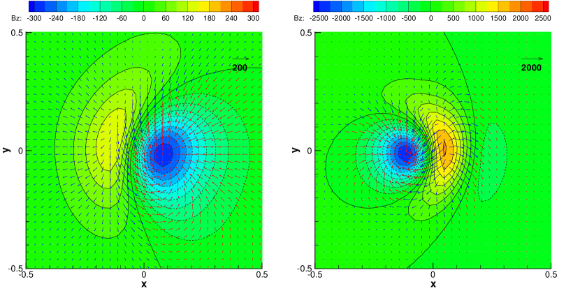
Figure 1: Vector magnetograms of the central region $x,y\in[-0.5,+0.5]$ for CASE LL1 (left) and CASE LL2 (right). The contours represent $B_{z}$. The tangential field is shown by the vectors with blue color in positive $B_{z}$ region and red in negative $B_{z}$ region.

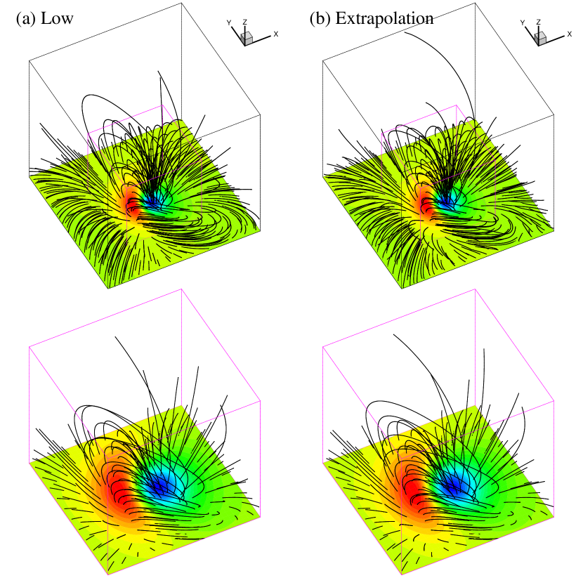
Figure 4: CASE LL1: magnetic field lines with contour of $B_{z}$ on the bottom surface. (a) the Low & Lou’s solution, (b) the extrapolation result. The bottom row enlarges the central region ($x,y\in[-0.5,+0.5]$ and $z\in[0,1]$) outlined by the small cube in the top row.

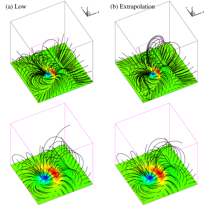
Figure 7: Same as Figure 4 but for CASE LL2.

where $A=P(\cos\theta)/r^{n}$ and $Q=aA^{1+1/n}$. The solution $P$ of Equation (16) is uniquely determined by two eigenvalues, $n$ and its number of nodes $m$ (Low & Lou, 1990; Amari et al., 2006). By arbitrarily positioning a plane in the space of the analytical fields, one obtains a different kind of test case, in which the plane represents the bottom-boundary condition for extrapolation of the overlaying fields. In this way the fields sliced by the plane show no more symmetry and thus benefit for a general testing of extrapolation. The position of the plane is characterized by two additional parameters, $l$ and $\Phi$. Here we choose two particular solutions characterized by the parameters ($n,m,l,\Phi$), which are respectively given by $n=1$, $m=1$, $l=0.3$ and $\Phi=\pi/4$ (referred to as CASE LL1), and $n=3$, $m=1$, $l=0.3$ and $\Phi=4\pi/5$ (CASE LL2). For both cases, the computational domain is $x,y\in[-1,+1]$ and $z\in[0,2]$ and discretized by uniform grid of $64\times 64\times 64$ (same as Paper I). The same test solutions are also used by works in the above references where more analyses of these fields can be found. The vector magnetograms for both cases at $z=0$ are shown in Figure 1 and their 3D field lines are shown in panels $(a)$ of Figures 4 and 7. Basically, non-potential fields occupy more volume in CASE LL1 than CASE LL2 and CASE LL2 is ‘more nonlinear’ with a larger $\alpha$ and stronger fields more concentrated near the center of the model volume. Since the solutions show rather smooth (small gradients) and relatively simple magnetic structures with their topologies roughly consistent with those of the potential fields based on the same LoS magnetograms, these tests can be regarded as preliminary tests for any new-developed NLFFF extrapolation methods before facing to more stringent cases or realistic magnetograms.

3.2 The van Ballegooijen Reference Model

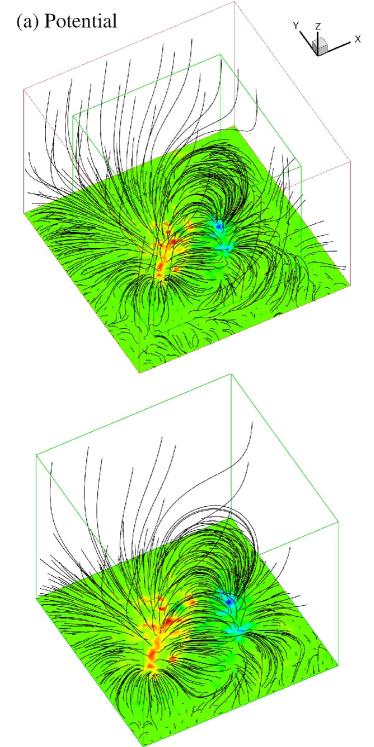
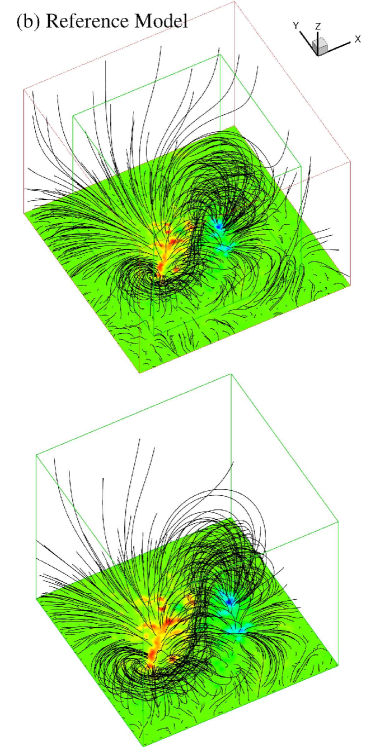
Figure 3: The van Ballegooijen reference model: magnetic field lines with contour of $B_{z}$ on the bottom surface. The field lines shown are traced from footpoints equally spaced at the bottom surface. (a) the initial potential field, (b) the final near-force-free reference model. The bottom row enlarges the central region outlined by the small cube in the top row.

The van Ballegooijen reference model is adopted from Paper II for a more stringent and realistic testing of our code. By this reference model, it is possible to mimic the analysis of real observational data while still knowing the properties of the field to be modeled. This model field is constructed by initially inserting an S-shaped flux bundle into a potential field associated with active region AR 10814 (see panel (a) of Figure 3), and then relaxing the unbalanced system to a near force-free state using van Ballegooijen’s magneto-frictional code in spherical geometry (van Ballegooijen et al., 2000; van Ballegooijen, 2004). Furthermore, an upward force was applied to the field at the lower boundary during the relaxation process to mimic the effect of magnetic buoyancy in the photoshpere, and thus achieve more realistic magnetic fields between photospheric and chromospheric heights in the model. Finally, by coordinate transformation and interpolation from the original spherical geometry, magnetic fields in a Cartesian box of $320\times 320\times 258$ pixels centered on the active region is extracted as the final reference model. The final near-force-free field are drawn in panel (b) of Figure 3, which contains several interesting topological features including a coronal null and its associated separatrix surface, and the S-shaped flux bundle surrounded by a quasi-separatrix layer (please see more details in Paper II). Compared with the initial potential field, the magnetic topology near the bottom is significantly modified by the low-lying flux rope, which challenges the extrapolation much more than the Low and Lou cases. Because of extra force presented at the bottom, this reference model can be used for tests of extrapolations from either the ‘chromospheric’ or the ‘photospheric’ magnetograms, by providing the NLFFF code with data at $z=z_{2}$ or $z=z_{0}$ ($z$ is the height in the model, e.g., $z_{0}$ is the base of the reference model). For the ‘chromospheric’ case, the boundary data used is largely force-free which is consistent with the extrapolation method, while the ‘photospheric’ case is more forced and thus represents a more realistic magnetogram of observation. It should be stressed that the van Ballegooijen reference model is not strictly force-free in the whole model box, even above the chromosphere, due to the implementation of the magneto-frictional method and some other numerical errors. It is demonstrated that in the model the residual forces of at least $5\%$ of magnetic-pressure force are present up to height of $z_{30}$, which are consistent with what is known of forces on the Sun, making the model a realistic, solar-like test case for the extrapolation codes.

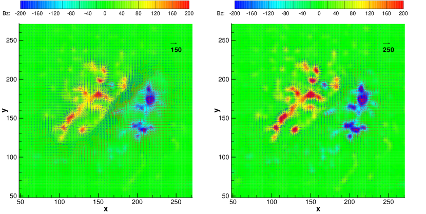
Figure 2: Vector magnetograms of the central $224^{2}$ pixels for chromospheric case (left) and preprocessed photospheric case (right). The contours represent $B_{z}$ with a saturation level of $\pm 200$ G. The tangential field is shown by the vectors (plotted at every second grid point) with blue color in positive $B_{z}$ region and red in negative $B_{z}$ region.

As done in Paper II, we will test our code by both the chromospheric and photospheric cases. For the photospheric case which is inconsistent with force-free assumption, we only examine the code with the photospheric magnetogram preprocessed by method of Wiegelmann & Neukirch (2006). The magnetograms of both test cases are plotted in Figure 2, which show a significant shearing along the polarity inversion line (PIL).

4 Metrics

For a detailed analysis of the extrapolation fields, a suite of metrics introduced in (Schrijver et al., 2006) are computed. These metrics compare either local characteristics including vector magnitudes and directions at each point or the global energy content. They are respectively the vector correlation $C_{\rm vec}$

$$C_{\rm vec}\equiv\sum_{i}\mathbf{B}_{i}\cdot\mathbf{b}_{i}/(\sum_{i}|\mathbf{B}_{i}|^{2}\sum_{i}|\mathbf{b}_{i}|^{2}),$$ (18)

the metric $C_{\rm CS}$ based on the Cauchy-Schwarz inequality

$$C_{\rm CS}\equiv\frac{1}{M}\sum_{i}\frac{\mathbf{B}_{i}\cdot\mathbf{b}_{i}}{|\mathbf{B}_{i}||\mathbf{b}_{i}|},$$ (19)

the normalized and mean vector error $E_{\rm n}^{\prime}$, $E_{\rm m}^{\prime}$

$$E_{\rm n}\equiv\sum_{i}|\mathbf{b}_{i}-\mathbf{B}_{i}|/\sum_{i}|\mathbf{B}_{i}|;E_{\rm n}^{\prime}=1-E_{\rm n},$$ (20)

$$E_{\rm m}\equiv\frac{1}{M}\sum_{i}\frac{|\mathbf{B}_{i}-\mathbf{b}_{i}|}{|\mathbf{B}_{i}|};E_{\rm m}^{\prime}=1-E_{\rm m},$$ (21)

where $\mathbf{B}_{i}$ and $\mathbf{b}_{i}$ denote the input field (the Low & Lou’s solution or the van Ballegooijen reference model in this paper) and the extrapolated field, respectively, $i$ denotes the indices of the grid points and $M$ is the total number of grid points involved. As can be seen, an exact extrapolation will have all the metrics equal to unity in such definitions, and the closer to unity means the better extrapolation and vice versa. Detailed descriptions for these metrics can be found in (Amari et al., 2006; Schrijver et al., 2006; Valori et al., 2007). Another very important parameter for comparing the extrapolation is the free energy of magnetic field. It is measured by the ratio of extrapolated energy to the potential energy using the same magnetogram,

$$E/E_{\rm pot}=\frac{\sum_{i}|{\mathbf{B}}_{i}|^{2}}{\sum_{i}|({\mathbf{B}}_{\rm pot})_{i}|^{2}},$$ (22)

It is common to measure the force-freeness and divergence-freeness of the extrapolation using the current-weighted sine metric CWsin and divergence metric $\langle|f_{i}|\rangle$ (Metcalf et al., 2008; Schrijver et al., 2008; DeRosa et al., 2009; Canou & Amari, 2010), which are defined by Wheatland et al. (2000) as

$${\rm CWsin}\equiv\frac{\sum_{i}|\mathbf{J}_{i}|\sigma_{i}}{\sum_{i}|\mathbf{J}_{i}|};\sigma_{i}=\frac{|\mathbf{J}_{i}\times\mathbf{B}_{i}|}{|\mathbf{J}_{i}||\mathbf{B}_{i}|}$$ (23)

and

$$\langle|f_{i}|\rangle=\frac{1}{M}\sum_{i}\frac{(\nabla\cdot\mathbf{B})_{i}}{6|{\mathbf{B}}_{i}|/\Delta x}$$ (24)

where $\Delta x$ is the grid spacing. Both of the metrics are normalized with the former focused on the directional deviation between the currents and the field lines and the latter on the relative value of residual divergence. These two metrics are equal to zero for an exact force-free field, and hence the smaller these metrics are, the better the extrapolation is.

In addition to the above metrics, we also introduce another pair of metrics to evaluate the degree of convergence towards the divergence-free and force-free state. For the first one, we note that a nonzero $\nabla\cdot\mathbf{B}$ (i.e., the magnetic monopole) introduces to the system an unphysical force ${\mathbf{F}}={\mathbf{B}}\nabla\cdot\mathbf{B}$ parallel to the field line (Dellar, 2001). To evaluate the effect of this unphysical force to the numerical computation, the metric $E_{\nabla\cdot\mathbf{B}}$ is defined as the average ratio of this force to the magnetic-pressure force

$$E_{\nabla\cdot\mathbf{B}}=\frac{1}{M}\sum_{i}\frac{|\mathbf{B}_{i}(\nabla\cdot\mathbf{B})_{i}|}{|\nabla(|{\mathbf{B}}|^{2}/2)_{i}|}.$$ (25)

Similarly, the second metric $E_{\nabla\times\mathbf{B}}$ measures the effect of the residual Lorentz force in the same way

$$E_{\nabla\times\mathbf{B}}=\frac{1}{M}\sum_{i}\frac{|{\mathbf{J}}_{i}\times{\mathbf{B}}_{i}|}{|\nabla(|{\mathbf{B}}|^{2}/2)_{i}|}.$$ (26)

Unlike the metrics of CWsin and $\langle|f_{i}|\rangle$ which mainly characterize the geometric properties of the field, these two metrics directly measure the physical action of the residual divergence and Lorentz force on the system in the actual numerical computation. This is important for checking of the NLFFF solution if it is used to initialize any MHD simulations.

For the all metrics above, the first four are more rigid since they are involved without any type of derivatives, while the other metrics may be unreliable for comparison with results from different papers due to the specific numerical realization of the derivatives (for example, different orders of numerical differentiation or different configurations of computational grid, e.g., cell-centered or staggered). In the present work, the second-order central difference is used for evaluating all the derivatives associated with the divergence, curl, and gradient operators, although the spatial derivatives can be directly obtained from the CESE method.

5 Results

In this section, we present the results of extrapolation for the benchmark models. The results are also compared with some results reported in Paper I, II and (Valori et al., 2007).

5.1 Low and Lou’s Force Free Field

5.1.1 CASE LL1

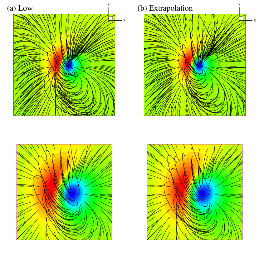
Figure 5: CASE LL1: same as Figure 4, but projected onto the $x$–$y$ planes.

Results for CASE LL1 are given in Figure 4, Figure 5, Table 1 and Table 2. In Figure 4, we show the same selected field lines in 3D view for the extrapolation results and the reference solution, which are traced from foot-points evenly rooted at the lower boundary. In the central region of core fields (i.e., $x,y\in[-0.5,+0.5]$ and $z\in[0,1]$, enlarged in the bottom row of the figures), the MHD result is highly in agreement with Low & Lou’s solution, as can be seen from the high similarity of most of the field lines. Such agreement is demonstrated quantitatively by the metrics in Table 1. The first three metrics are very close to $1$ with error of $<5\%$ and even the most sensitive metric $E_{m}^{\prime}$ has an error below $10\%$. In Table 1 we also compare with the best result by Wiegelmann’s code (Wiegelmann, 2004) reported in Paper I and extrapolation by Valori et al. (2007). Our result for the central region, although only specified the lower boundary, still reaches the level of the best extrapolation that using information of Low & Lou’s solution on all six boundaries. This may be due to the fact that this test case is close to potential field hence a fixed side and top boundary conditions can rarely impact the central extrapolation. The influence of the boundary conditions is more explicitly shown by comparison of the metrics for the entire domain. Now the Wiegelmann’s extrapolation still performs perfectly with all four metrics extremely close to unity, while our result and the Valori’s perform less exactly, but still satisfactory. Like other results in the Table, our extrapolation also recovered the energy content very precisely, especially for the central region; furthermore the metrics evaluating the force-freeness and divergence-freeness are rather small and close to the reference values which is caused by discretization error. All these shows that extrapolation of very high accuracy can be achieved by our implementation, at least for the present, relatively easy test case.

In the Valori’s implementation of the magneto-frictional method (Valori et al., 2007), a fourth-order numerical scheme is used with many layers of ghost mesh and a high-order polynomial extrapolation of the fields is adopted on the side and top boundaries. However by comparing our result with Valori’s, it is interesting to note that our implementation performs better although our numerical scheme is second-order method without any ghost layers and the boundaries are simply fixed. In this test, the boundary effect can be neglected as said (while in the following test of CASE LL2, we will see the effect of different treatments of these boundaries). Then we concluded that the better performance is due to the merit of using a better solver, i.e., CESE method combined with the magnetic splitting algorithm which can gain additional accuracy.

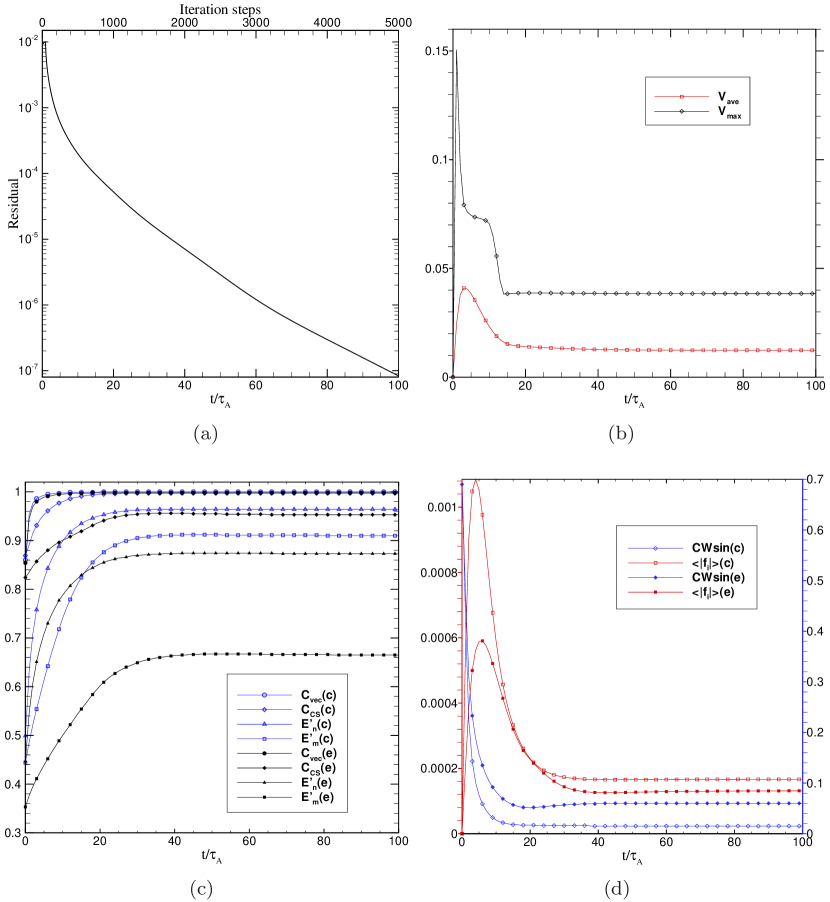
Figure 6: CASE LL1: The history of the relaxation to force-free equilibrium. (a) Evolution of residual ${\rm res}({\mathbf{B}})$ with time (or the iteration steps); (b) evolution of the maximum and average velocity; and (c), (d) evolution of the metrics for the central region (marked by (c)) and the entire volume (marked by (e)).

We finally give a study of the convergence of the extrapolation. In Figure 6 we shows the history of the system relaxing to the final force-free equilibrium, including the residual of temporal evolution of the magnetic field

$${\rm res}^{n}({\mathbf{B}})=\sqrt{\frac{1}{3}\sum_{\delta=x,y,z}\frac{\sum_{i}(B_{i\delta}^{n}-B_{i\delta}^{n-1})^{2}}{\sum_{i}(B_{i\delta}^{n})^{2}}}$$ (27)

(where $n$ denotes the iteration steps), the evolution of the velocity and the metrics. The system converged very fast from a initial residual of $10^{-2}$ to value under $10^{-7}$ with time of $100\tau_{A}$ (about $5000$ iteration steps, see panel (a) of Figure 6). The evolution of the plasma velocity indicates that a static equilibrium is reached as expected with a rather small residual velocity $\sim 0.01$ which is only on the order of the numerical error $O(\Delta x^{2})$ of the CESE solver. All the metrics plotted in the figure converged after $40\tau_{A}$ (about 2000 iteration steps), when the residual is on the order of $10^{-5}$. Note that the metric $f_{i}$ of $\nabla\cdot\mathbf{B}$, like the plasma velocity, first climbs to a relatively high level ($\sim 0.01$, see panel (d)) and then drops to the level of discretization errors. In principle the divergence-free constraint of ${\mathbf{B}}$ should be fulfilled throughout the evolution, at least close to level of discretization error. However, a ideally dissipationless induction equation Equation (6) with divergence-free constraint can preserve the magnetic connectivity, which makes the topology of the magnetic field unchangeable (Wiegelmann, 2008) unless a finite resistivity is included for allowing reconnection and changing of the magnetic topology (Roumeliotis, 1996). In the present implementation in which no resistivity is included in the induction equation, a break of $\nabla\cdot\mathbf{B}$ constraint in the initial evolution process (indicated by the climb of metric $f_{i}$) can thus produce a change in the magnetic topology (also note that a numerical diffusion can help to topology adjustment in addition).

Model	$C_{\rm vec}$	$C_{\rm CS}$	$E_{\rm n}^{\prime}$	$E_{\rm m}^{\prime}$	$E/E_{\rm pot}$	CWsin	$\langle|f_{i}|\rangle$
For the central region
Low	1.000	1.000	1.000	1.000	1.242	0.014	$0.94\times 10^{-4}$
Our result	1.000	0.997	0.964	0.912	1.241	0.015	$1.67\times 10^{-4}$
Wiegelmann∗	1.00	1.00	0.97	0.96	1.26
Valori∗∗	0.999	0.99	0.95	0.87	1.23	0.009
Potential	0.858	0.869	0.498	0.443	1.000
For the entire domain
Low	1.000	1.000	1.000	1.000	1.294	0.014	$0.56\times 10^{-4}$
Our result	0.998	0.955	0.873	0.662	1.282	0.060	$1.31\times 10^{-4}$
Wiegelmann∗	1.00	1.00	0.98	0.98	1.31	0.070
Valori∗∗	0.994	0.86	0.80	0.51	1.28	0.019
Potential	0.852	0.824	0.446	0.353	1.000

Table 1: CASE LL1: Metrics for the central and entire regions. The superscript $*$ denotes the reported results in Table I and Table II of Paper I, and $**$ denotes the reported results by Valori et al. (2007).

Model	$E_{\nabla\times\mathbf{B}}$	$E_{\nabla\cdot\mathbf{B}}$
For the central region
Low	0.007	0.005
Our result	0.010	0.008
For the entire region
Low	0.003	0.002
Our result	0.024	0.005

Table 2: CASE LL1: Metrics of $E_{\nabla\times\mathbf{B}}$ and $E_{\nabla\cdot\mathbf{B}}$

5.1.2 CASE LL2

Now we present the result of the second test CASE LL2 which is more difficult than the first one. Compared with CASE LL1, this case is more non-potential and nonlinear with relatively larger gradient of fields. Although considering of this, our extrapolation still gives satisfactory result that is as good as the best result in Paper I (see the first four metrics shown and compared in Table 3). It is also quite encouraging that our result for the central region is close to Valori’s which is computed with fourth-order numerical scheme. Figure 7 and 8 demonstrate qualitatively the consistence with the Low and Lou’s reference solution. The energy contents are very well reproduced for both the central region and the entire domain.

By comparing the metrics of the entire domain, we find that our result scores worse than the Valori’s, especially shown by $E^{\prime}_{\rm m}$. The reason for this is twofold. Firstly, a high-order scheme can characterize the large gradient much more accurately than 2nd-order scheme and thus the fourth-order scheme by Valori et al. (2007) shows its advantages for this test case with larger gradient than CASE LL1 (the high-order accuracy can be also achieved by mesh refinement other than improving the order of the numerical scheme. As demonstrated in our previous work (Jiang et al., 2011), a refined grid of $128\times 128\times 100$ with the CESE scheme gave much more accurate result with the most sensitive metric even reaching $0.166$). Secondly, our implementation simply fixed the artificial boundaries (i.e., the lateral and top faces), which obviously make the system over-determined. In the present test case the final field is very non-potential, hence the boundary values deviate from the initial conditions significantly. A fixed boundary condition will tie the field lines that pass through the boundary, which would otherwise freely cross the boundary since this boundary is a non-existing interface in the realistic corona. This line-tied condition thus hinders the system from relaxing to a true force-free state. The metric of CWsin demonstrates clearly that the field is less force-free than the Valori’s result. The boundary effect can be seen visually from some field lines close to the lateral boundaries shown in the figures (e.g., see the distortion of field lines at the lower left coroners of panel (b) in Figure 7 and 8). Also caused by the boundary effect, the field for the entire domain (${\rm CWsin}=0.060$) is thus less force-free than the central region (${\rm CWsin}=0.047$). In a full MHD simulation, this boundary effect can be minimized by using a so-called non-reflecting boundary conditions based on characteristic decomposition of the full MHD system (Wu et al., 2001, 2006; Hayashi, 2005; Feng et al., 2010; Jiang et al., 2011). However for the present form of magneto-frictional equation, the characteristic method is no more valid because of the eigen degeneration of the non-hyperbolic system. In such situation, a natural choice of modeling the non-reflecting boundary is to use linear or high-order extrapolation, just as done by Valori et al. (2007). Fortunately, field configuration like this Low & Lou case with the entire volume very non-potential is not usually found in observed magnetograms, and by choosing a model box significant larger than the core non-potential region, a simply fixed boundary values of the initial potential field is still sufficient for most extrapolations, for example, test cases in the next section.

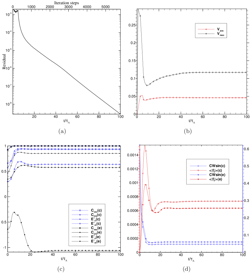
Figure 9: Same as Figure 6 but for CASE LL2.

Figure 9 shows that the convergence speed is even faster than case LL1. The residual of the magnetic field reaches the order of $10^{-7}$ with only $\sim 3200$ iterations at $60\tau_{A}$. The evolution speed of the magnetic field is also demonstrated by magnitude of the plasma velocity, which is larger than that of case LL1. At about $30\tau_{A}$, all the metrics converged with the corresponding residual of magnetic field on the order of $10^{-5}$. This and the preceding cases, shows that generally the iteration can be stopped when ${\rm res}^{n}({\mathbf{B}})<10^{-6}$ since after that temporal change of the magnetic field can be neglected actually.

Model	$C_{\rm vec}$	$C_{\rm CS}$	$E_{\rm n}^{\prime}$	$E_{\rm m}^{\prime}$	$E/E_{\rm pot}$	CWsin	$\langle|f_{i}|\rangle$
For the central region
Low	1.000	1.000	1.000	1.000	1.099	0.036	$3.14\times 10^{-4}$
Our result	0.999	0.933	0.938	0.636	1.114	0.047	$7.35\times 10^{-4}$
Wiegelmann∗	1.00	0.91	0.92	0.66	1.14
Valori∗∗	0.999	0.95	0.96	0.75	1.11	0.015
Potential	0.923	0.661	0.572	0.299	1.000
For the entire domain
Low	1.000	1.000	1.000	1.000	1.100	0.035	$2.17\times 10^{-4}$
Our result	0.999	0.574	0.852	-1.060	1.115	0.060	$6.35\times 10^{-4}$
Wiegelmann∗	1.00	0.57	0.86	-0.25	1.14
Valori∗∗	0.999	0.64	0.88	-0.01	1.11	0.027
Potential	0.921	0.346	0.465	-0.639	1.000

Table 3: Same as Table 1 but for LL CASE2. The superscript $*$ denotes the reported results in Table I and Table II of Paper I, and $**$ denotes the reported results by Valori et al. (2007).

Model	$E_{\nabla\times\mathbf{B}}$	$E_{\nabla\cdot\mathbf{B}}$
For the central region
Low	0.011	0.008
Our result	0.026	0.024
For the entire region
Low	0.004	0.003
Our result	0.025	0.013

Table 4: CASE LL2: Metrics of $E_{\nabla\times\mathbf{B}}$ and $E_{\nabla\cdot\mathbf{B}}$

5.2 The van Ballegooijen Reference Field

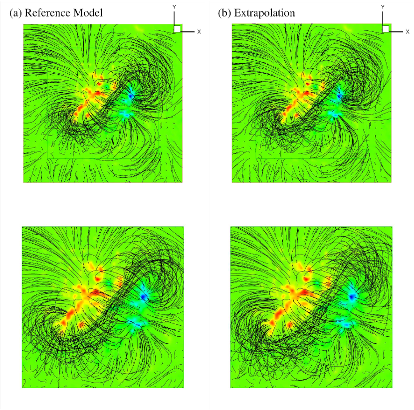
Figure 11: Chromospheric test case of the van Ballegooijen reference model: same as Figure 10, but projected onto the $x$–$y$ planes.

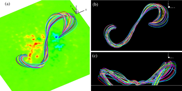
Figure 12: The van Ballegooijen reference model: different views of the fluxrope. (a) 3D view, (b) projection on the $x$–$y$ plane and (c) on the $x$–$z$ plane with the white line denoting the bottom. Since the middle of the fluxrope lies very close to the bottom, the $z$ scale in panel (c) is enlarged twice for a better view of the field lines.

We first perform the extrapolation of the chromospheric case, which provides a largely force-free magnetogram without any preprocessing. Figure 10 shows the 3D field lines of extrapolation and the reference model for a side-by-side comparison. The field lines shown are traced from foot-points equally spaced at the bottom surface. We specially adjusted the figures to an approximately same orientation as Paper II on purpose of visual comparison with those results by other codes. The same field lines are also projected on the $x$–$y$ plane in Figure 11. As shown from a overall view of the figures, the extrapolation reproduced quite well the basic magnetic topology including the low-lying S-shaped field-line bundle, and the overlying magnetic arcade that straddles the flux rope. For a confirmation of presence of the flux rope in the extrapolation, we select a set of field lines of the S-shaped bundle and plot them using different colors in Figure 12 with different perspectives. It clearly shows that the flux rope are qualitatively recovered, encouraging us that the code can be used to handle such relatively complex test cases. The extrapolated flux rope is weakly twisted and its core fields basically lies along the bottom PIL, showing a highly shear with respect to the overlying arcades.

In Table 5 we give a quantitative evaluation and comparison of the result with those reported in Paper II. To minimize the (side and top) boundary effects, the metrics are applied to the central region of $(x,y)\in[48,271]\times[48,271]$ with two different heights: $z\in[2,61]$ for focusing on the low-lying flux rope and $z\in[2,225]$ for including also the surrounding potential-like field. This is done in the same way as in Paper II and the results along with the first three preferable results in Paper II are presented. Note that some metrics (e.g., the $C_{\rm CS}$ and CWsin) for the reference and potential models differs slightly from those shown in Paper II, which may be due to different precisions (i.e., single or double precision) used in the numerical computation.

As shown by Table 5, the extrapolation performs very well with errors only of $\sim 2\%$ for the first two metrics. These metrics, however, are not sensitive indicator of extrapolation accuracy (Valori et al., 2007) and thus all the methods in Paper II give these metrics within the same level, even including the potential field. By the more sensitive metrics $E_{\rm n}$ and $E_{\rm m}$, we find that our result for $z\in[2,225]$ is identical with the best result performed by Wiegelmann. For the lower height, the deviations of these metrics with the best result are smaller than $<2\%$ (note that these deviations can be also partially introduced by the different precisions in the numerical computation). This comparison encourages us further of the success of our implementation. Our result also gives the energy metrics very close to the reference values, showing a good recovering of the free energy content, which is particularly important for coronal field extrapolation. Finally the CWsin metric behaves a bit worse than the first five metrics if compared with the Wiegelmann’s result, but it still scores better than the following results by Wheatland and Valori.

The last two metrics $E_{\nabla\times\mathbf{B}}$ and $E_{\nabla\cdot\mathbf{B}}$ (shown in Table 7), both of which are non-zero but in a very low level, mean that the reference model is very close to force-free and divergence-free but never exact as expected (see Section 5.2). Again, our results present values very similar to those of the reference model. Note that although both CWsin and $E_{\nabla\times\mathbf{B}}$ measure the degree of force-free, the former depends more strongly on the high-current regions (Valori et al., 2007) while the latter is not. Hence CWsin for both heights gives nearly the same value of $0.1$, while $E_{\nabla\times\mathbf{B}}$ gives significant larger value $0.06$ for the lower domain ($z\in[2,61]$) than value $0.018$ for the full domain ($z\in[2,225]$), which shows that the residual forces are mainly presented in the lower region. By these two metrics, we demonstrate that our code can minimize the residual forces into a very low values and fulfill the divergence-free condition well.

In Table 5, the result with the multigrid-type algorithm is also presented, which is performed on a three-grid sequence ($80\times 80\times 64$, $160\times 160\times 128$ and the full resolution $320\times 320\times 256$). We found that this result (with multigrid algorithm) behaves a little bit worse compared with the result without multigrid algorithm. This is due to the additional numerical errors of $\nabla\times\mathbf{B}$ and $\nabla\cdot\mathbf{B}$ introduced by interpolating field from coarser to finer grid, which thus results in a little bit larger values of CWsin and $\langle|f_{i}|\rangle$ than those without multigrid algorithm. Without the multigrid algorithm, the magnetic field splitting form can avoid such numerical errors by using a zero ${\mathbf{B}}_{1}$ initially and thus performs better. However in spite of such small disadvantage, the multigrid algorithm is still encouraged to be adopted since its reward is a significant reduce of the computing time (e.g., for the present test case, we find that using of the multigrid algorithm saves approximately two-thirds of the CPU time).

Now we present the results for the photospheric case with preprocessed magnetogram. The preprocessing procedure can remove the net forces of the photospheric magnetogram and hence provide the extrapolation code a more consistent lower boundary condition than the raw magnetogram. In Paper II, both cases with the raw and preprocessed photospheric magnetograms are tested, and it is found that the preprocessed case gives a significantly better result than the raw case in which the flux rope is not reproduced at all. This demonstrated that the preprocessing procedure is necessary for those extrapolation codes. Besides, the smoothing involved in the preprocessing also benefits the extrapolation code which is based on numerical finite-difference.

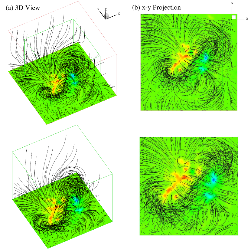
Figure 13: Photospheric test case of the van Ballegooijen reference model: magnetic field lines with contour of $B_{z}$ on the bottom surface. (a) 3D view and (b) $x$–$y$ plane projection of the extrapolation result. The bottom row enlarges the central region outlined by the small cube in the top row.

Our result are given in Figure 13 and Table 6. The field lines shows that the overall structure including the flux rope is still recovered qualitatively, but partially. By careful comparison with the reference or the chromospheric cases, the difference is also evident, e.g., the bundle of S-shaped lines is much thinner in the present case, which seems that many field lines have not reconnected fully to form a entire S. The quantitative comparison also demonstrates that the extrapolation quality is a bit worse than chromospheric case, especially shown by the CWsin and $E_{\nabla\times\mathbf{B}}$ metrics (nearly twice of those of the chromospheric case). It means the extrapolated field is farther away from the exactly force-free state than the chromospheric case. The free energy is also underestimated much, as the results in Paper II. This is because the preprocessing does not recover a force-free magnetogram that is entirely consistent with the reference model. Still, it is worthwhile noting that our result again reaches the same level of the best in Paper II, and some of the metrics, including the most sensitive one $E_{\rm m}$, perform even better than Wiegelmann’s.

Model	$C_{\rm vec}$	$C_{\rm CS}$	$E_{\rm n}^{\prime}$	$E_{\rm m}^{\prime}$	$E/E_{\rm pot}$	CWsin	$\langle|f_{i}|\rangle$
For $z\in[2,225]$
Reference	1.000	1.000	1.000	1.000	1.343	0.107	$1.02\times 10^{-4}$
Our result	0.995	0.978	0.885	0.734	1.337	0.133	$1.11\times 10^{-4}$
Our resultM	0.993	0.975	0.868	0.712	1.357	0.142	$1.32\times 10^{-4}$
Wiegelmann∗	1.00	0.99	0.89	0.73	1.34	0.11
Wheatland∗	0.95	0.98	0.79	0.70	1.21	0.15
Valori∗	0.98	0.98	0.84	0.71	1.25	0.15
Potential	0.852	0.952	0.687	0.665	1.000
For $z\in[2,61]$
Reference	1.000	1.000	1.000	1.000	1.361	0.103	$1.33\times 10^{-4}$
Our result	0.995	0.989	0.923	0.883	1.348	0.125	$1.58\times 10^{-4}$
Our resultM	0.993	0.979	0.902	0.825	1.366	0.129	$1.74\times 10^{-4}$
Wiegelmann∗	1.00	0.99	0.94	0.89	-	0.11
Wheatland∗	0.95	0.95	0.79	0.76	-	0.15
Valori∗	0.98	0.96	0.86	0.81	-	0.15
Potential	0.847	0.901	0.660	0.678	1.000

Table 5: The van Ballegooijen reference model: metrics for extrapolation of the chromospheric case. The superscript M denotes the multigrid-type algorithm is used for speeding up of the extrapolation and the superscript $*$ denotes the reported results in Table 3 and Table 4 of Paper II.

Model	$C_{\rm vec}$	$C_{\rm CS}$	$E_{\rm n}^{\prime}$	$E_{\rm m}^{\prime}$	$E/E_{\rm pot}$	CWsin	$\langle|f_{i}|\rangle$
For $z\in[2,225]$
Reference	1.000	1.000	1.000	1.000	1.531	0.107	$1.02\times 10^{-4}$
Our result	0.970	0.968	0.783	0.679	1.146	0.257	$2.29\times 10^{-4}$
Wiegelmann∗	0.98	0.97	0.77	0.65	1.18	0.26
Wheatland∗	0.88	0.96	0.69	0.65	1.03	0.11
Potential	0.850	0.945	0.659	0.636	1.000
For $z\in[2,61]$
Reference	1.000	1.000	1.000	1.000	1.559	0.103	$1.33\times 10^{-4}$
Our result	0.970	0.980	0.800	0.791	1.149	0.230	$3.45\times 10^{-4}$
Potential	0.845	0.891	0.629	0.646	1.000

Table 6: The van Ballegooijen reference model: metrics for extrapolation of the photospheric case. The superscript $*$ denotes the reported results in Table 3 of Paper II.

Model	$E_{\nabla\times\mathbf{B}}$	$E_{\nabla\cdot\mathbf{B}}$
For $z\in[2,225]$
Reference	0.018	0.004
Our result of the chromospheric case	0.023	0.005
Our result of the photospheric case	0.048	0.015
For $z\in[2,61]$
Reference	0.060	0.010
Our result of the chromospheric case	0.072	0.014
Our result of the photospheric case	0.132	0.040

Table 7: The van Ballegooijen reference model: metrics of $E_{\nabla\times\mathbf{B}}$ and $E_{\nabla\cdot\mathbf{B}}$.

6 Conclusions

As a viable way of study magnetic field in the corona, the NLFFF extrapolation also needs a considerable effort to be devoted for its numerical realization. In this paper, a new numerical implementation of NLFFF extrapolation is presented based on the MHD relaxation method and the CESE-MHD code. Our implementation outstands for the following aspects.

1. The magneto-frictional approach that is designed for speeding the relaxation of the MHD system (Roumeliotis, 1996; Valori et al., 2007) is novelly realized by the high-performance CESE scheme on a grid without any type of ghost zone or buffer layer.

2. The accuracy is further improved by firstly utilizing the magnetic splitting form (Tanaka, 1994) for NLFFF methods to totally avoid the numerically random errors involved with the initial input.

3. Multi-method control, i.e., the diffusive and convection term, of numerical magnetic monopoles is employed for effectively reducing the divergence error.

4. The vector magnetogram is inputted at the bottom boundary in the way of time-linearly modifying the potential field to matching the magnetogram and other artificial boundaries are just fixed as the initial potential values, which makes our implementation much easier than other MHD relaxation methods (e.g., those by Roumeliotis (1996) and Valori et al. (2007)).

5. The code is highly parallelized with the help of PARAMESH toolkit and performed on the share-memory parallel computer. It can be readily realized with the AMR technique and applied to very high-resolution magnetogram in the near future. The multigrid-type algorithm is also incorporated into the code to speedup the computation as recommended.

We have examined the capability of the method by several reference solutions of NLFFF that can be served as a suite of benchmark tests for any NLFFF extrapolation code. These test cases consist of the classic half-analytic force-free fields by Low & Lou (Low & Lou, 1990) and the much more stringent and solar-like reference solution by van Ballegooijen (2004). The results show that our method are successful and versatile for extrapolations of either the relatively simple cases or the rather complex cases which need significant rebuilding of the magnetic topology, e.g., the flux rope. We also compute a suite of metrics to quantitatively analyze the results, and shows that the solutions are extrapolated with high accuracies which are very close to and even surpass the best results by Wiegelmann (2004) from comparison of the metrics. This demonstrated that, at least in computation accuracy, our code performs as good as the best one of state-of-the-art (the computing time of the code, however, is difficult to be compared because the hardwares are different). In addition, we introduced a pair of metrics for assessment of the divergence-freeness and force-freeness of the extrapolation, $E_{\nabla\cdot\mathbf{B}}$ and $E_{\nabla\times\mathbf{B}}$, which further demonstrated that our code can fulfill the solenoidal constraint well and minimize the Lorentz force to the same level of the reference values.

The success of our implementation encouraged us that with a good solver, the MHD relaxation approach can also extrapolate the NLFFF as accurately as other good-performance algorithms, like the weighting optimization method. This confirms again that the way of implementation of the methods plays the same important role as their underlying approach. It is especially worthwhile pointing out that, as also noted by (Wiegelmann, 2008), the MHD relaxation approach has a great advantage over other methods: any available time-dependent MHD code can be adjusted for NLFFF extrapolations, which thus saves the major effort that should be made to develop a new code from scratch for a special method. We are also inspired by Valori et al. (2007), who show that a higher order scheme can significantly advance the extrapolation. In our project, an arbitrary high order CESE scheme is under development and is expected to be used for future improvement of our implementation.

Recently, more critical tests of extrapolation codes have been performed by Schrijver et al. (2008) and DeRosa et al. (2009) based on vector magnetograms of AR 10930 and 10953 from Hinode/SOT and observed coronal loops. It is found that the Grad-Rubin-style current-field iteration implemented by Wheatland (2006) surpassed the Wiegelmann (2004)’s code that performs best in the benchmark tests, and basically the results by different methods are very inconsistent with each other. This shows that the idealized tests are unable to assess the code’s ability to deal with various uncertainties or errors in the real magnetograms and more critical assessment of the code using realistic vector magnetograms is also planned in our future work.

The present extrapolation in Cartesian geometry is often limited to relatively local areas, e.g., a single active region without any relationship with others. However, the active regions cannot be isolated since they generally interact with neighboring ARs or overlaying large scale fields. It is also pointed out that the fields of view in Cartesian box are often too small to properly characterize the entire relevant current system (DeRosa et al., 2009). To study the connectivity between multi-active regions and extrapolate in a larger field of view, it is necessary to take into account the curvature of the Sun’s surface by extrapolation in spherical geometry partly or even entirely, i.e., including the global corona (Wiegelmann, 2007; Tadesse et al., 2011a, b). Moreover, a global NLFFF extrapolation can also avoid any lateral artificial boundaries which are inescapable and cause issues in Cartesian codes. We are now on the way of developing a global NLFFF code for the new era of routinely observation of the global vector magnetogram (which will be opened by SDO/HMI). Recently in a project of constructing a data-driven MHD model for the global coronal evolution, we have established the CESE method on a so-called Yin-Yang overlapping grid in spherical geometry (Kageyama & Sato, 2004). This implementation, combined with our present NLFFF code, will make the realization of a global NLFFF extrapolation very viable if provided with the global vector magnetogram. The Yin-Yang grid is composed of two identical component grids that are combined in a complemental way to cover an entire spherical surface with partial overlap on their boundaries. Each component grid is a low latitude part of the latitude-longitude grid without the pole and hence the grid spacing on the sphere surface is quasi-uniform. In this way, we can avoid the problem of grid convergence or grid singularity at both poles which will otherwise arise if an entire spherical-coordinate grid is used, as Wiegelmann (2007) has pointed out. However, up to now, there is no suitable test case used for the global NLFFF extrapolation other than the simple axially-symmetric Low & Lou cases. Most recently, Contopoulos et al. (2011) give a variety of global near force-free solutions by a force-free electrodynamics code, using solely the radial magnetogram. Their solutions, however, are not unique to the same radial magnetogram, but depends on the initial conditions and on the particular approach to steady-state . Anyway, we believe their solutions can be used as much more realistic and solar-like tests for global NLFFF codes than the semi-analytic solutions. In our future work, we will develop and test a new global NLFFF code by the global force-free solutions from (Contopoulos et al., 2011).

Appendix A The specific form of Equation (11)

$$\mathbf{F}=\left(\begin{array}[]{c}\vskip 6.0pt plus 2.0pt minus 2.0pt\cr{\mathbf{B}}_{1}\cdot{\mathbf{B}}_{1}/2-B_{1x}^{2}-(B_{0x}B_{1x}+B_{1x}B_{0x})+{\mathbf{B}}_{0}\cdot{\mathbf{B}}_{1}\\ \vskip 6.0pt plus 2.0pt minus 2.0pt\cr-B_{1x}B_{1y}-(B_{0x}B_{1y}+B_{1x}B_{0y})\\ \vskip 6.0pt plus 2.0pt minus 2.0pt\cr-B_{1x}B_{1z}-(B_{0x}B_{1z}+B_{1x}B_{0z})\\ \vskip 6.0pt plus 2.0pt minus 2.0pt\cr 0\\ \vskip 6.0pt plus 2.0pt minus 2.0pt\cr v_{x}B_{y}-v_{y}B_{x}\\ \vskip 6.0pt plus 2.0pt minus 2.0pt\cr v_{x}B_{z}-v_{z}B_{x}\\ \vskip 6.0pt plus 2.0pt minus 2.0pt\cr 0\\ \vskip 6.0pt plus 2.0pt minus 2.0pt\cr 0\\ \vskip 6.0pt plus 2.0pt minus 2.0pt\cr 0\end{array}\right);$$ (A10)

$$\mathbf{G}=\left(\begin{array}[]{c}\vskip 6.0pt plus 2.0pt minus 2.0pt\cr-B_{1y}B_{1x}-(B_{0y}B_{1x}+B_{1y}B_{0x})\\ \vskip 6.0pt plus 2.0pt minus 2.0pt\cr{\mathbf{B}}_{1}\cdot{\mathbf{B}}_{1}/2-B_{1y}^{2}-(B_{0y}B_{1y}+B_{1y}B_{0y})+{\mathbf{B}}_{0}\cdot{\mathbf{B}}_{1}\\ \vskip 6.0pt plus 2.0pt minus 2.0pt\cr-B_{1y}B_{1z}-(B_{0y}B_{1z}+B_{1y}B_{0z})\\ \vskip 6.0pt plus 2.0pt minus 2.0pt\cr v_{y}B_{x}-v_{x}B_{y}\\ \vskip 6.0pt plus 2.0pt minus 2.0pt\cr 0\\ \vskip 6.0pt plus 2.0pt minus 2.0pt\cr v_{y}B_{z}-v_{z}B_{y}\\ \vskip 6.0pt plus 2.0pt minus 2.0pt\cr 0\\ \vskip 6.0pt plus 2.0pt minus 2.0pt\cr 0\\ \vskip 6.0pt plus 2.0pt minus 2.0pt\cr 0\end{array}\right);$$ (A20)

$$\mathbf{H}=\left(\begin{array}[]{c}\vskip 6.0pt plus 2.0pt minus 2.0pt\cr-B_{1z}B_{1x}-(B_{0z}B_{1x}+B_{1z}B_{0x})\\ \vskip 6.0pt plus 2.0pt minus 2.0pt\cr-B_{1z}B_{1y}-(B_{0z}B_{1y}+B_{1z}B_{0y})\\ \vskip 6.0pt plus 2.0pt minus 2.0pt\cr{\mathbf{B}}_{1}\cdot{\mathbf{B}}_{1}/2-B_{1z}^{2}-(B_{0z}B_{1z}+B_{1z}B_{0z})+{\mathbf{B}}_{0}\cdot{\mathbf{B}}_{1}\\ \vskip 6.0pt plus 2.0pt minus 2.0pt\cr v_{z}B_{x}-v_{x}B_{z}\\ \vskip 6.0pt plus 2.0pt minus 2.0pt\cr v_{z}B_{y}-v_{y}B_{z}\\ \vskip 6.0pt plus 2.0pt minus 2.0pt\cr 0\\ \vskip 6.0pt plus 2.0pt minus 2.0pt\cr 0\\ \vskip 6.0pt plus 2.0pt minus 2.0pt\cr 0\\ \vskip 6.0pt plus 2.0pt minus 2.0pt\cr 0\end{array}\right);$$ (A30)

$${\mathbf{F}}_{\nu}=(0,0,0,\mu\nabla\cdot\mathbf{B}_{1},0,0,0,0,0)^{T};$$

$${\mathbf{G}}_{\nu}=(0,0,0,0,\mu\nabla\cdot\mathbf{B}_{1},0,0,0,0)^{T};$$

$${\mathbf{H}}_{\nu}=(0,0,0,0,0,\mu\nabla\cdot\mathbf{B}_{1},0,0,0)^{T};$$ (A31)

$${\mathbf{S}}=(-\nu\rho v_{x},-\nu\rho v_{y},-\nu\rho v_{z},v_{x}\nabla\cdot\mathbf{B}_{1},v_{y}\nabla\cdot\mathbf{B}_{1},v_{z}\nabla\cdot\mathbf{B}_{1},0,0,0)$$ (A32)

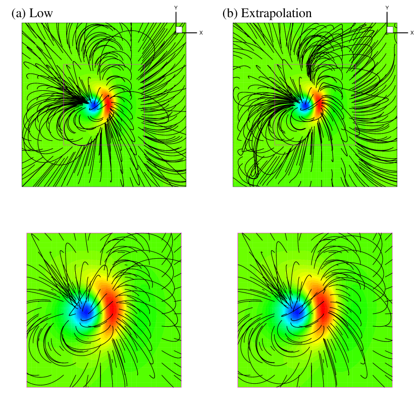
Figure 8: Same as Figure 5 but for CASE LL2.

Figure 10: Chromospheric test case of the van Ballegooijen reference model: magnetic field lines with contour of $B_{z}$ on the bottom surface. (a) the reference model, (b) the extrapolation result. The bottom row enlarges the central region outlined by the small cube in the top row.

References

- Abbett & Fisher (2003) Abbett, W. P. & Fisher, G. H. 2003, ApJ, 582, 475
- Abbett et al. (2004) Abbett, W. P., Mikić, Z., Linker, J. A., McTiernan, J. M., Magara, T., & Fisher, G. H. 2004, J. Atmos. Sol.-Terr. Phys., 66, 1257
- Altschuler & Newkirk (1969) Altschuler, M. D. & Newkirk, G. 1969, Sol. Phys., 9, 131
- Aly (1989) Aly, J. J. 1989, Sol. Phys., 120, 19
- Amari et al. (1997) Amari, T., Aly, J. J., Luciani, J. F., Boulmezaoud, T. Z., & Mikic, Z. 1997, Sol. Phys., 174, 129
- Amari et al. (2006) Amari, T., Boulmezaoud, T. Z., & Aly, J. J. 2006, A&A, 446, 691
- Amari et al. (1999) Amari, T., Boulmezaoud, T. Z., & Mikic, Z. 1999, A&A, 350, 1051
- Aschwanden (2005) Aschwanden, M. J. 2005, Physics of the Solar Corona. An Introduction with Problems and Solutions (2nd edition), ed. Aschwanden, M. J.
- Canou & Amari (2010) Canou, A. & Amari, T. 2010, ApJ, 715, 1566
- Chang (2002) Chang, S. C. 2002, AIAA Paper, 2002-3890
- Chodura & Schlueter (1981) Chodura, R. & Schlueter, A. 1981, J. Comput. Phys., 41, 68
- Contopoulos et al. (2011) Contopoulos, I., Kalapotharakos, C., & Georgoulis, M. K. 2011, Sol. Phys., 269, 351
- Dedner et al. (2002) Dedner, A., Kemm, F., Kröner, D., Munz, C., Schnitzer, T., & Wesenberg, M. 2002, J. Comput. Phys., 175, 645
- Dellar (2001) Dellar, P. J. 2001, J. Comput. Phys., 172, 392
- DeRosa et al. (2009) DeRosa, M. L., Schrijver, C. J., Barnes, G., Leka, K. D., Lites, B. W., Aschwanden, M. J., Amari, T., Canou, A., McTiernan, J. M., Régnier, S., Thalmann, J. K., Valori, G., Wheatland, M. S., Wiegelmann, T., Cheung, M. C. M., Conlon, P. A., Fuhrmann, M., Inhester, B., & Tadesse, T. 2009, ApJ, 696, 1780
- Feng et al. (2006) Feng, X., Hu, Y., & Wei, F. 2006, Sol. Phys., 235, 235
- Feng et al. (2007) Feng, X., Zhou, Y., & Wu, S. T. 2007, ApJ, 655, 1110
- Feng et al. (2010) Feng, X. S., Yang, L. P., Xiang, C. Q., Wu, S. T., Zhou, Y. F., & Zhong, D. K. 2010, ApJ, 723, 300
- Grad & Rubin (1958) Grad, H. & Rubin, H. 1958, in 2nd Int. Conf. Peac. Uses of Atom. Energy, Vol. 31, 386
- Hayashi (2005) Hayashi, K. 2005, ApJS, 161, 480
- He & Wang (2008) He, H. & Wang, H. 2008, J. Geophys. Res., 113, 5
- He et al. (2011) He, H., Wang, H., & Yan, Y. 2011, J. Geophys. Res., 116, 1101
- Hoeksema (1984) Hoeksema, J. T. 1984, PhD thesis, Stanford Univ., CA.
- Inhester & Wiegelmann (2006) Inhester, B. & Wiegelmann, T. 2006, Sol. Phys., 235, 201
- Inoue et al. (2011) Inoue, S., Kusano, K., Magara, T., Shiota, D., & Yamamoto, T. T. 2011, ApJ, 738, 161
- Jiang et al. (2011) Jiang, C. W., Feng, X. S., Fan, Y. L., & Xiang, C. Q. 2011, ApJ, 727, 101
- Jiang et al. (2012) Jiang, C. W., Cui, S. X., & Feng, X. S. 2012, Computers & Fluids, 54, 105
- Jiang et al. (2010) Jiang, C. W., Feng, X. S., Zhang, J., & Zhong, D. K. 2010, Sol. Phys., 267, 463
- Kageyama & Sato (2004) Kageyama, A. & Sato, T. 2004, Geochemistry, Geophysics, Geosystems, 5, 9005
- Linker et al. (1999) Linker, J. A., Mikić, Z., Biesecker, D. A., Forsyth, R. J., Gibson, S. E., Lazarus, A. J., Lecinski, A., Riley, P., Szabo, A., & Thompson, B. J. 1999, J. Geophys. Res., 104, 9809
- Low & Lou (1990) Low, B. C. & Lou, Y. Q. 1990, ApJ, 352, 343
- MacNeice et al. (2000) MacNeice, P., Olson, K. M., Mobarry, C., de Fainchtein, R., & Packer, C. 2000, Comput. Phys. Commun., 126, 330
- Marder (1987) Marder, B. 1987, J. Comput. Phys., 68, 48
- McClymont et al. (1997) McClymont, A. N., Jiao, L., & Mikic, Z. 1997, Sol. Phys., 174, 191
- Metcalf et al. (2008) Metcalf, T. R., DeRosa, M. L., Schrijver, C. J., Barnes, G., van Ballegooijen, A. A., Wiegelmann, T., Wheatland, M. S., Valori, G., & McTtiernan, J. M. 2008, Sol. Phys., 247, 269
- Mikić et al. (1999) Mikić, Z., Linker, J. A., Schnack, D. D., Lionello, R., & Tarditi, A. 1999, Phys. Plasmas, 6, 2217
- Mikic & McClymont (1994) Mikic, Z. & McClymont, A. N. 1994, in Astronomical Society of the Pacific Conference Series, Vol. 68, Solar Active Region Evolution: Comparing Models with Observations, ed. K. S. Balasubramaniam & G. W. Simon, 225–+
- Nakagawa (1974) Nakagawa, Y. 1974, ApJ, 190, 437
- Nakamizo et al. (2009) Nakamizo, A., Tanaka, T., Kubo, Y., Kamei, S., Shimazu, H., & Shinagawa, H. 2009, J. Geophys. Res.(Space Phys.), 114, A07109
- Powell et al. (1999) Powell, K. G., Roe, P. L., Linde, T. J., Gombosi, T. I., & de Zeeuw, D. L. 1999, J. Comput. Phys., 154, 284
- Roumeliotis (1996) Roumeliotis, G. 1996, ApJ, 473, 1095
- Sakurai (1981) Sakurai, T. 1981, Sol. Phys., 69, 343
- Sakurai (1989) Sakurai, T. 1989, Space Sci. Rev., 51, 11
- Schrijver et al. (2006) Schrijver, C. J., De Rosa, M. L., Metcalf, T. R., Liu, Y., McTiernan, J., Régnier, S., Valori, G., Wheatland, M. S., & Wiegelmann, T. 2006, Sol. Phys., 235, 161
- Schrijver et al. (2008) Schrijver, C. J., DeRosa, M. L., Metcalf, T., Barnes, G., Lites, B., Tarbell, T., McTiernan, J., Valori, G., Wiegelmann, T., Wheatland, M. S., Amari, T., Aulanier, G., Démoulin, P., Fuhrmann, M., Kusano, K., Régnier, S., & Thalmann, J. K. 2008, ApJ, 675, 1637
- Song et al. (2006) Song, M. T., Fang, C., Tang, Y. H., Wu, S. T., & Zhang, Y. A. 2006, ApJ, 649, 1084
- Tadesse et al. (2011a) Tadesse, T., Wiegelmann, T., Inhester, B., & Pevtsov, A. 2011a, Sol. Phys., 167
- Tadesse et al. (2011b) —. 2011b, A&A, 527, A30
- Tanaka (1994) Tanaka, T. 1994, J. Comput. Phys., 111, 381
- Tóth & Roe (2002) Tóth, G. & Roe, P. L. 2002, J. Comput. Phys., 180, 736
- Valori et al. (2007) Valori, G., Kliem, B., & Fuhrmann, M. 2007, Sol. Phys., 245, 263
- Valori et al. (2005) Valori, G., Kliem, B., & Keppens, R. 2005, A&A, 433, 335
- van Ballegooijen (2004) van Ballegooijen, A. A. 2004, ApJ, 612, 519
- van Ballegooijen et al. (2007) van Ballegooijen, A. A., Deluca, E. E., Squires, K., & Mackay, D. H. 2007, J. Atmos. Sol.-Terr. Phys., 69, 24
- van Ballegooijen et al. (2000) van Ballegooijen, A. A., Priest, E. R., & Mackay, D. H. 2000, ApJ, 539, 983
- Wang et al. (2011) Wang, A. H., Wu, S. T., Tandberg-Hanssen, E., & Hill, F. 2011, ApJ, 732, 19
- Welsch et al. (2004) Welsch, B. T., Fisher, G. H., Abbett, W. P., & Regnier, S. 2004, ApJ, 610, 1148
- Wheatland (2004) Wheatland, M. S. 2004, Sol. Phys., 222, 247
- Wheatland (2006) —. 2006, Sol. Phys., 238, 29
- Wheatland et al. (2000) Wheatland, M. S., Sturrock, P. A., & Roumeliotis, G. 2000, ApJ, 540, 1150
- Wiegelmann (2004) Wiegelmann, T. 2004, Sol. Phys., 219, 87
- Wiegelmann (2007) —. 2007, Sol. Phys., 240, 227
- Wiegelmann (2008) —. 2008, J. Geophys. Res., 113, 3
- Wiegelmann & Neukirch (2006) Wiegelmann, T. & Neukirch, T. 2006, A&A, 457, 1053
- Wu et al. (1990) Wu, S. T., Sun, M. T., Chang, H. M., Hagyard, M. J., & Gary, G. A. 1990, ApJ, 362, 698
- Wu et al. (2009) Wu, S. T., Wang, A. H., Gary, G. A., Kucera, A., Rybak, J., Liu, Y., Vrśnak, B., & Yurchyshyn, V. 2009, Adv. Space Res., 44, 46
- Wu et al. (2006) Wu, S. T., Wang, A. H., Liu, Y., & Hoeksema, J. T. 2006, ApJ, 652, 800
- Wu et al. (2001) Wu, S. T., Zheng, H., Wang, S., Thompson, B. J., Plunkett, S. P., Zhao, X. P., & Dryer, M. 2001, J. Geophys. Res., 106, 25089
- Yan & Li (2006) Yan, Y. & Li, Z. 2006, ApJ, 638, 1162
- Yan & Sakurai (2000) Yan, Y. & Sakurai, T. 2000, Sol. Phys., 195, 89
- Yang et al. (1986) Yang, W. H., Sturrock, P. A., & Antiochos, S. K. 1986, ApJ, 309, 383
- Zhang et al. (2006) Zhang, M., John Yu, S., Henry Lin, S., Chang, S., & Blankson, I. 2006, J. Comput. Phys., 214, 599