Study of single-lobed circular polarization profiles in the quiet sun

Abstract

The existence of asymmetries in the circular polarization (Stokes V) profiles emerging from the solar photosphere is known since the 1970s. These profiles require the presence of a velocity gradient along the line of sight, possibly associated with gradients of magnetic field strength, inclination and/or azimuth. We have focused our study on the Stokes V profiles showing extreme asymmetry in the from of only one lobe. Using Hinode spectropolarimetric measurements we have performed a statistical study of the properties of these profiles in the quiet sun. We show their spatial distribution, their main physical properties, how they are related with several physical observables and their behavior with respect to their position on the solar disk. The single lobed Stokes V profiles occupy roughly 2% of the solar surface. For the first time, we have observed their temporal evolution and have retrieved the physical conditions of the atmospheres from which they emerged using an inversion code implementing discontinuities of the atmospheric parameters along the line of sight. In addition, we use synthetic Stokes profiles from 3D magnetoconvection simulations to complement the results of the inversion. The main features of the synthetic single-lobed profiles are in general agreement with the observed ones, lending support to the magnetic and dynamic topologies inferred from the inversion. The combination of all these different analysis suggests that most of the single-lobed Stokes V profiles are signals coming from magnetic flux emergence and/or submergence processes taking place in small patches in the photospheric of the quiet sun.

1. Introduction

Stokes parameters are used to characterize the polarization state of light: the Stokes I parameter tells us about the intensity, Q and U about the linear polarization and V about the circular polarization (Rees et al., 1989; Landi Degl’Innocenti, 1992; del Toro Iniesta, 2003). The variation of these parameters across a spectral line are called Stokes profiles. When the light beam comes from a static atmosphere, the Stokes I, Q and U profiles are symmetric functions, and Stokes V is antisymmetric showing two lobes of opposite signs with respect to the central wavelength. However, the Stokes V signals coming from the solar atmosphere rarely are purely antisymmetric, i.e., the two lobes are different either in shape, in amplitude or in area. The asymmetry of the Stokes V is generally described in terms of the difference between the amplitudes (or the areas) of each lobe normalized to their sum. The asymmetry in the Stokes V profile requires a velocity gradients in the atmosphere where the radiation is coming from (Illing et al. 1975; Auer & Heasley 1978; Landolfi & Landi Degl’Innocenti 1996 among others). In case of extreme asymmetries, one of the lobes of Stokes V is missing. These are referred as single-lobed Stokes V profiles. Such large asymmetries cannot be explained with a velocity gradient alone, and require gradients of the magnetic field vector.

In this paper we present a detailed analysis of the single-lobed Stokes V profiles observed in the quiet sun. These profiles show only one lobe, or two lobes with one reduced by a very large extent. Profiles of this type were first described by Sigwarth et al. (1999) and studied in detail by Sigwarth (2001) and Grossmann-Doerth et al. (2000). The former author studied the amount of blue-only and red-only single-lobed Stokes V profiles in the quiet sun. Sigwarth (2001) observed a ratio of blue-only to red only profiles of 4:1. He associated the blue-only profiles with magnetic structures exhibiting downflows whereas the red-only profiles seemed to be related to upflows. He used a large scan area, so he could not observed the temporal evolution of these signals. Therefore, although he proposed several scenarios, he could not explain the phenomena behind them.

To explain the existence of Stokes V profiles with strong asymmetry several theoretical models featuring large gradients in velocity and magnetic field have been suggested. If the stratification is simple enough, the blue-only lobe in the Stokes V profile is stronger (weaker) than the red lobe if the LOS velocity gradient as a function of depth is opposite (equal) to the magnetic field strength gradient (Illing et al., 1975; Auer & Heasley, 1978). Steiner (2000) proposed that single-lobed profiles can be produced when the line of sight passes through a magnetopause, i.e., a separatrix layer dividing the atmosphere vertically in two regions with different magnetic fields. Magnetopauses occur frequently in the solar atmosphere. Examples are the canopies created by expanding flux tubes in the network and the interfaces between different magnetic components in sunspot penumbrae (see Grossmann-Doerth et al., 2000; Steiner, 2000; Schlichenmaier et al., 1998). Steiner (2000) suggested that a tiny loop expanding towards the upper layers, being smaller than the spatial resolution, could create single-lobed Stokes V profiles if the expansion of the magnetic field lines in one of the footpoints of the loop is larger than in the other. In this case, the footpoint related with the large expansion would create asymmetric Stokes V profiles (without extreme asymmetry), while the footpoint with normal expansion would produce symmetric Stokes V profiles of opposite sign. The superposition of both profiles - as a result of limited spatial resolution - would cancel one of the lobe and, therefore, the observed profile would be a single-lobed Stokes V profile(see Figure 9 in Steiner 2000). Sanchez Almeida et al. (1996) synthesized single-lobed Stokes V profiles under the MISMA assumption. This type of unusual Stokes V profiles has been related with upward traveling shocks driven by an aborted convective collapsed (Bellot Rubio et al., 2001). They have been observed in convective collapse events that take place simultaneously in the photosphere and chromosphere (Fischer et al., 2009). Narayan & Scharmer (2010) found that Stokes V profiles with large amplitude asymmetries are exclusively located at the boundary between regions with small-scale abnormal granulation and much larger normal-looking granules. Recently, Viticchié et al. (2011) have successfully inverted single-lobed Stokes V profiles located either in the neutral line of opposite polarity patches or in the very quiet sun.

The identification of the physical mechanism(s) behind the single-lobed circular polarization profiles observed in the quiet sun represents both an observational and a theoretical challenge. Here, we use all the tools at our disposal to shed light on these intriguing profiles. We analyze a large number of spectropolarimetric measurements taken by Hinode at high spatial resolution in order to determine the observational properties of the profiles in a statistically significant way (Sections 2-6) and to investigate their temporal evolution (Section 7). We also apply Stokes inversions to the data based on models with discontinuities along the line of sight (Section 8). The inversions successfully reproduce the observed spectra. Finally, we search for single-lobed Stokes V profiles in 3D magnetoconvection simulations of the quiet sun and study the magnetic and dynamic topologies associated with them. Our combined approach allows us to draw a general picture of this phenomenon. A complementary analysis of single-lobed profiles in 3D magnetoconvection simulations has been performed recently by Viticchié & Vitas (2012).

2. Data

The data used in this paper were obtained by the Spectro-Polarimeter (SP) located in the Focal Plane Package (FPP) of the Solar Optical Telescope (SOT, Tsuneta et al. 2008) on board the Hinode satellite (Kosugi et al., 2007). This instrument, hereafter referred to as Hinode SOT/SP measures the four Stokes parameters of the Fe I lines at 6301 and 6302 Å  with spectral sampling of 21.5 $m$Å . The spatial scale can be 0.15″ or 0.30″ for the X direction (perpendicular to the slit direction) and 0.16″ or 0.32″ for the Y direction (parallel to the slit). For the first time, these data allow to investigate the four Stokes parameters of the single-lobed Stokes V profiles under seeing-free conditions and with unmatched spatial resolution.

We use 72 data sets spanning a wide range of observational conditions: exposure time (1.6, 3.2, 4.8, 8.0, 9.6 and 12.6 s); signal to noise ratio (between 500 and 1000, calculated as the inverse of the standard deviation, $\sigma$); position on the solar disk (56 maps with 1.00 $>\mu>$ 0.75, 8 maps with 0.75 $>\mu>$ 0.50 and 8 maps with 0.50 $>\mu>$ 0); and spatial scale (as mentioned above). Our data sets contain scans of large quiet sun regions and narrower scans with typical widths of 2-10 granules, for a variety of heliocentric distances. Table LABEL:latabla in the appendix summarizes the basic parameters of the different observing runs. All the analyzed profiles have been calibrated using Solarsoft routines.

3. Data Analysis

To identify single-lobed profiles, we have developed a code that checks the shape of the Stokes V spectra and flags the ones that have only one lobe. This code was applied to almost $5.2\times 10^{7}$ pixels corresponding to the 72 selected observations. The code looks into the shape of the Stokes V profiles, and takes into account the following constraints:

• The maximum (minimum) signal must be greater (smaller) than 4 (-4) times $\sigma$.

• At least three wavelength points must show signals above (below) the 4$\sigma$ (-4$\sigma$) threshold.

• Simultaneously, the other lobe and the minimum (maximum) of the whole Stokes V profile must be greater (less) than -3$\sigma$ (3$\sigma$).

• In the continuum, the circular polarization signal can never exceed $\pm$ 3$\sigma$.

If these conditions are satisfied by one of the lobes of Fe I 6301 Å or 6302 Å  then the profile is flagged as a single-lobed profile. For Fe I 6301 Å, the blue lobe goes from 6301.18$\pm 0.02$ Å ($\lambda_{b}$) to 6301.50 Å ($\lambda_{c}$), and the red lobe from 6301.50 Å to 6301.82 Å ($\lambda_{r}$). For Fe I 6302 Å, the blue lobe is between 6302.17 Å ($\lambda_{b}$) and 6302.49 Å ($\lambda_{c}$), while the red one goes from 6302.49 Å to 6302.82 Å($\lambda_{r}$).

In order to relate the location of the single-lobed Stokes V profiles with physical parameters, we have extracted several line parameters from the observed Stokes spectra:

• Stokes I map: for the slit reconstructed Stokes I map we used 8 spectral positions on the continuum, located between 6303.12 Å and 6303.27 Å.

• Stokes V map: in this case we used 36 spectral positions located on the blue wing of the Stokes V profiles of Fe I 6302 Å, roughly from 6301.72 Å to 6302.49 Å.

• Doppler velocities, determined through line bisectors. We use the line bisector at the 70% intensity level (the midpoint between the flanks of the line at that intensity) minus the line core wavelength position of the average quiet sun profile. The difference is converted into velocity and expressed in km s^-1. Thus, the zero velocity is given by the local average quiet sun profile

• The mean circular polarization degree is calculated as: $MCPD=(\int_{\lambda_{0}}^{\lambda_{1}}{\frac{|V(\lambda)|d\lambda}{I(\lambda)}})/(\lambda_{1}-\lambda_{0})$

• The mean linear polarization degree is calculated as: $MLPD=(\int_{\lambda_{0}}^{\lambda_{1}}{\frac{\sqrt{Q^{2}(\lambda)+U^{2}(\lambda)}}{I(\lambda)}d\lambda})/(\lambda_{1}-\lambda_{0})$

• The mean total polarization degree is calculated as: $MTPD=(\int_{\lambda_{0}}^{\lambda_{1}}{\frac{\sqrt{Q^{2}(\lambda)+U^{2}(\lambda)+V^{2}(\lambda)}}{I(\lambda)}d\lambda})/(\lambda_{1}-\lambda_{0})$

The integrals are evaluated from $\lambda_{0}$=6301.29 Å to $\lambda_{1}$=6301.71 Å in the case of Fe I 6301 Å, and from $\lambda_{0}$=6302.27 Å to $\lambda_{1}$=6302.70 Å for Fe I 6302 Å. These wavelength intervals cover all the relevant polarization signals, avoiding the contribution of the continuum.

4. Spatial distribution of single-lobed Stokes V profiles

In Figure 1 we show examples of blue-only and red-only Stokes V profiles (left and right panels, respectively). There are clear Stokes Q and U signals associated with the blue-only profiles, indicating the existence of inclined magnetic fields with respect to the line of sight. Furthermore, both Q and U are asymmetric profiles. For the red-lobe profile the Stokes Q and U signals are much smaller and appear to consist of a single lobe on the red wing of the lines. The continuum intensities are larger than 1 and around 1 for the blue-only and red-only profiles, respectively. This means that the blue-only profile corresponds to a bright structure in the intensity map.

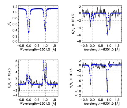
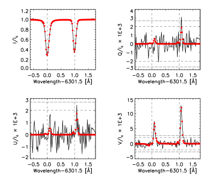
Figure 1.— Stokes profiles emerging for the locations marked with the yellow crosses in the left panel of Figure 2. The horizontal lines display the thresholds used by the code to identify the single-lobed Stokes V profiles, i.e., $\pm 3\sigma$ and $\pm 4\sigma$. The four left panels (clockwise starting from top left: Stokes I, Q, V, and U) correspond to a case of blue-only profile and the four right panels correspond to a case of red-only profile. The dots represent the best fit profiles found by the inversion code SIRJUMP (see section 8).

Let us concentrate on a small region ($21\arcsec\times 16.5\arcsec$) of one large scan for showing the location of the blue-only and red-only profiles. The measurements displayed in Figure 2, were taken on September 24, 2007 at 20 h 42 min UT. The spatial sampling is $0.15\arcsec$ and $0.16\arcsec$ in X and Y direction respectively; the exposure time is 12.8 s and its location is the center of the solar disk ($\mu\sim 1.0$). Figure 2 shows that the blue-only profiles tend to be located in the outer part of the granules (blue contours). In contrast, the red only profiles are mainly located in the intergranular area (red contours).

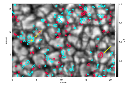
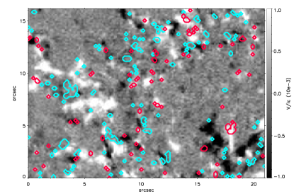
Figure 2.— Left: Stokes I map shown in grey scale (part of the observation taken on September, 24 2007) with the blue-only and red-only profile locations indicated with the respective contours. The yellow crosses pointed by yellow arrows mark the positions of the pixels whose Stokes V profiles are shown in Figure 3 and 4. Right: Stokes V map.

Figures 3 and 4 show the spatial distribution of the Stokes V profiles in an area of 9 px $\times$ 9 px (1.35″$\times$ 1.44″) around the yellow crosses displayed in Figure 2. For reference, the border of granules are represented by the black intensity contour. Figure 3 makes it clear that there are no regular Stokes V profiles of opposite polarities close to the blue-only profiles. This suggests that the processes leading to the absence of one lobe in Stokes V are not related to the horizontal mixing of atmospheres with different physical conditions. In the case of red-only profiles (Figure 4), there are some asymmetric Stokes V signals of opposite polarity nearby, but they seem to be related with the expansion of the granular edge in the intergranular lane (see Section 7).

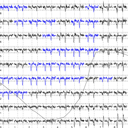
Figure 3.— Stokes V profiles shown for each pixel around the yellow cross located at the position (4,8) of Figure 2. The horizontal lines mark $\pm 3\sigma$ (dot-dot-dot-dashed lines) and $\pm 4\sigma$ (dot-dashed lines) levels. The vertical dashed lines indicate the nominal position of the core of the Fe I 6301 Å and 6302 Å lines. The contours indicate the visible edge of the granule. This region corresponds to an area with blue-only profiles.

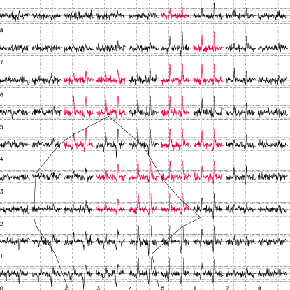
Figure 4.— Same as Figure 3, for the Stokes V profiles around the yellow cross located at (18,5) in Figure 2. This region corresponds to an area with red-only profiles.

5. Physical characterization of their locations

We have examined the location of the single-lobed profiles on the Stokes I and V maps, dopplergrams, and polarization degree maps to understand the general behavior with respect to the intensity, velocity and magnetic field. In addition, we have calculated histograms for these physical quantities. For clarity, we only show the previously selected case, and the mean ranges for these quantities using the full data set.

The left panel of the first row in Figure 5 shows the Stokes I map of the studied case. We have selected 5 interesting locations marked with numbers and arrows. At first glance, this figure tells us two interesting properties of the single-lobed Stokes V profiles: (i) The single-lobed profiles tend to appear in small patches. The red patches are very small and sometimes extend over one pixel only. By contrast, the blue patches are well-defined spatial structures, although they may look point-like too. (ii) The majority of red-only profiles are located in intergranular lanes. The blue-only profiles are very often sited on the outer part of the granules, sometimes in intergranular lanes, and in a few cases in the center of granules.

The right panel in the first row of Figure 5 displays the histogram of the intensity normalized to the quiet sun continuum. Although the distribution is rather broad -notice that the Y axis is displayed in logarithmic scale-, it is clear that the blue-only profiles are more correlated with the brighter structures than the red-only profiles. Except for the scans located very close to the limb, all the other data sets show this behavior. On average, the distribution associated with the blue-only profiles has the maximum at $1.05\pm 0.05I_{c}$ and spans the range $[0.85,1.20]\pm 0.05I_{c}$. For the red-only profiles the maximum is located at $0.95I_{c}\pm 0.05I_{c}$ and the range is $[0.85,1.10]\pm 0.05I_{c}$. The ranges are very similar in both cases, but the distribution of the red-only profiles is always located to the left (darker) in comparison to the blue-only profiles, as it is shown in Figure 5. Near the limb, the ranges in intensity are similar for red-only and blue-only profiles, and the maximum are for both cases located at $1.00\pm 0.05I_{c}$. Therefore, it is hard to distinguish where these profiles are located. This is a consequence of the low intensity contrast at the limb. In addition, one should keep in mind that observations close to the limb refer to higher layers of the solar atmosphere.

The dopplergram and the velocity distribution are shown in the second row of Figure 5. Similarly to the intensity distribution, the velocities associated with single-lobed Stokes V profiles show a broad range of variation, but there is a trend of the blue-only profiles to be associated with upflows (negative velocities). The red-only profiles tend to be associated with downflows (positive velocities). On average, the maximum of the velocity distribution for the blue-only profiles is -0.8 km s^-1, within the range [-2,+1] km s^-1. For the red-only profiles the maximum is 0.8 km s^-1, with values ranging from -1 to +2 km s^-1. Therefore, their velocities are roughly shifted +1 km s^-1 with respect to those of the blue-only profiles. For the single-lobed Stokes V profiles closer to the limb the ranges are [-2,+3] km s^-1 and [-2,+2] km s^-1 for the blue-only and red-only profiles, respectively. These results are in disagreement with Sigwarth (2001): On average, he associated both the blue-only and red-only profiles with downflows, although the former had stronger downflows than the latter.

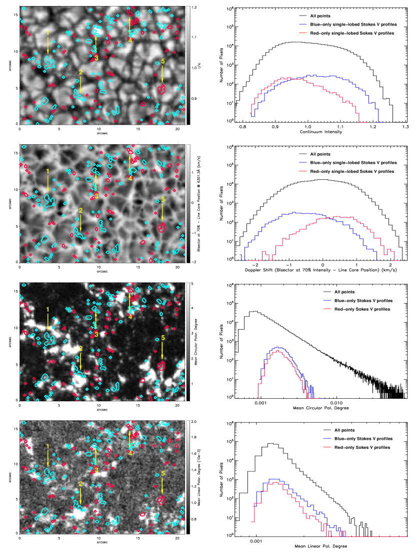
Figure 5.— Left column, from top to bottom: spatial distribution of single-lobed Stokes V profiles over-plotted on the intensity, Doppler shift, MCPD and MLPD maps shown in grey scale. The right columns show the corresponding histograms for the whole scan.

Now we describe the five locations marked in Figure 5 that we consider interesting to analyze in more detail. Locations #1 and #2 are two examples of large size patches. The first extends almost over the whole granule, while the second covers the outer part of two granules and the intergranular lanes. Location #1 sits in an upflow region (dark areas in the dopplergram shown in Figure 5); the lower part of location #2 is also in an upflow region, but most part of it is in a transition region with velocities close to zero (grey color in the dopplergram). Location #3 is just over the outer part of the granule with a high intensity and large upflows.

In the same figure, the locations #4 and #5 show red-only profiles. The former is located in an intergranular lane, with strong downflows (bright areas in the dopplergram). Location #5 is a structure nearly $2\arcsec\times 2\arcsec$ in size. It is over a transition region in the middle of two granules. It is not so well-defined as an intergranular region in the intensity map, but it is more evident in the dopplergram. In the dopplergram, this region is correlated with a narrow bright (downflow) intergranular lane and with the grey areas of the outer part of the neighboring granules.

Looking at the mean polarization degree maps we find other interesting properties of the single-lobed Stokes V profiles. The third and the fourth row of Figure 5 respectively show the MCPD and MLPD maps (left) and their distributions (right). Single-lobed profiles tend to be located at the periphery of magnetic flux concentrations showing strong linear and/or circular polarization signals. This fact can be seen at locations #1, #2 and #3, where the contours are surrounded by strong magnetic components. These locations are close to magnetic structures but not exactly on them. The locations #4 and #5 are partially over magnetic structures with weak signals in the polarization degree maps. This is the most common behavior for the single-lobed Stokes V profiles, as it can be seen in the distributions of the polarization degree shown in Figure 5. The mean circular polarization degree histogram follows a linear power law of index $-2.48$ in the range [0.0008,0.04]. However, for the blue-only and red-only profiles the mean circular polarization degree histogram follows a sharper linear power law of index $-6.02$ and $-6.49$ for blue-only and red-only profiles, respectively, both in the range [0.0015,0.005]. The mean linear polarization degree histogram follows a linear power law of index $-8.16$ in the range [0.0015,0.005]. In a similar manner, the mean linear polarization histogram for red-only and blue-only profiles follows a power law of index $-8.15$ and $-7.33$ respectively, in the range of [0.0015,0.003]. Both the blue-only and the red-only profiles are related with modest values of the longitudinal component and with the weaker transversal field components. In summary, the single-lobed Stokes V profiles are either close to strong magnetic structures -but not inside them- or over weak structures with both components of the magnetic field.

The locations of the single-lobed Stokes V profiles do not show a preference with the polarization sign of structures, i.e., these profiles appear with the same probability near positive and negative magnetic fields (see Stokes V map in the left panel in Figure 2).

Figure 6.— Intensity map showing the spatial distribution of single-lobed Stokes V profiles in quiet sun at the disk center. In the selected areas #1 and #4 these profiles are located around abnormal granulation patterns because of the presence of the network. The single-lobed Stokes V profile can also be seen in normal granulation, as in regions #2 and #3.

If we look in a larger area, as the one shown in Figure 6, we can see how the single-lobed Stokes V profiles are around abnormal granulation areas (as region #1 and #4) but also in normal granulation regions (as region #2 and #3). This observation contradicts the results obtained by Narayan & Scharmer (2010). Indeed, the single-lobed Stokes V profiles are in the borders of the network patches -usually showing abnormal granulation pattern in continuum images- but never inside them. In addition, the single-lobed Stokes V profiles are also present in the internetwork, where the granulation has normal properties.

Figures 7 and 8 show the MCPD and MLPD for the same area as in Figure 6. The large patches with strong signal form the network. The single-lobed Stokes V profiles are never located inside these patches. Rather, they surround the network and internetwork elements. The arrows mark the locations of several single-lobed Stokes V profiles showing both circular and linear polarization signals, i.e., where the magnetic field is inclined. Figure 9 shows the MCPD and MLPD maps in an area of roughly $5\arcsec\times 5\arcsec$ around the selected positions mark with arrows in Figures 7 and 8. As one can see, location #1 and #2 are in small patches with linear polarization signal and surrounded by network patches with strong circular polarization. Location #3 corresponds to an internetwork patch with strong linear polarization signal surrounded by small patches with weak circular polarization.

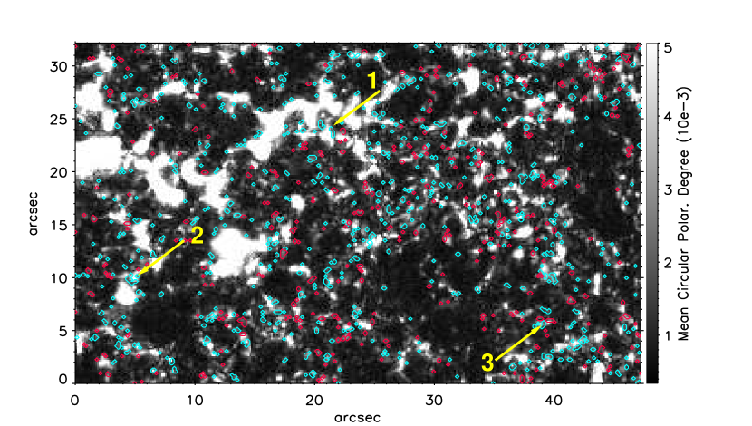
Figure 7.— MCPD map of the network and internetwork regions shown in Figure 6, with blue-only and red-only profiles in blue and red, respectively. The arrows mark locations where the blue-only and red-only profiles are either totally or partially located on structures with moderate strength of the longitudinal polarization signal.

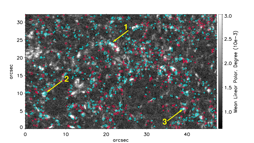
Figure 8.— MLPD map (grey scale) of the same area shown in Figure 6, where we over-plotted the blue-only and red-only profiles in blue and red contours. In this figure we selected several locations (again marked by arrows here) with significant longitudinal polarization signal. These places have also an large linear polarization signal.

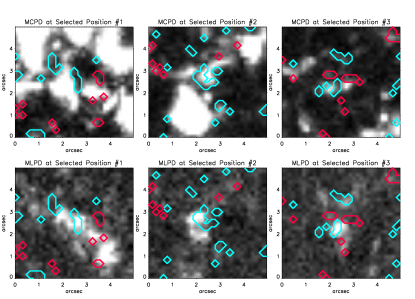
Figure 9.— Top: MCPD zoomed maps of the selected positions in Figure 7. Bottom: the same zoomed areas for the MLPD displayed in Figure 8. The three blue-only patches located in the center of the images have associated transversal polarization signal. The cases #1 and #3 are surrounded by structures with longitudinal component of the vector magnetic field. The case #2 has simultaneously both components of B. The thresholds for the MCPD and MLPD maps are respectively $5\times 10^{-3}$ and $3\times 10^{-3}$.

6. Center-to-limb variation

As mentioned above, we have examined 72 observing runs to search for single-lobed Stokes V profiles. Here, we present the behavior of these profiles with respect to their location on the solar disk. In Table LABEL:latabla we summarize the statistical properties of the profiles. The last 4 columns of the table give the following parameters: the signal to noise ratio (S/N); the percentage of blue-only profiles among the Stokes V profiles with absolute signal greater than $4\sigma$; the percentage of the red-only profiles, and the ratio between the blue-only and red-only profiles (annotated as B/R).

We have plotted the number of occurrences of the blue-only and red-only profiles taking into account their location on the solar disk and exposure times in Figure 10. The color of the points codes the exposure time. Sometimes, there is overlap between data points. For instance, at (1.0,1.6) there is a red point (12.8 s) that overlaps a pink point (9.6 s). The fraction of blue-only profiles in the disk-center is roughly 4%. The plot shows that the fraction of blue-only profiles decreases as the observation is made closer to the limb (roughly 1.6% near the limb). There is a decreasing trend in the fraction for the points of the same color as they are located closer to the limb (left side of the plot). This fact does not depend on the exposure time, i.e., the number of blue-only profile decreases in the full range of circular polarization signal, not only in the stronger ones (observed in the center of the solar disk with short exposure time), but also in the weaker ones (observed in the limb with longer exposure time).

In contrast, the fraction of red-only profiles remains fairly constant for different positions on the solar disk (roughly 2%). There is a slight increase of the green points, i.e., from 1.3% in the disk-center to 3.2% at $\mu\approx 0.46$ (corresponding to observations with exposure time of 1.6 s). If we pay attention to the other colored points, the overall impression is that the variation with the heliocentric distance of the number of occurrence is nearly constant.

The ratio of blue-only to red-only profiles is shown in Figure 12. This quantity drops from about 2-4 near the disk center to 0.5 as the limb is approached. This strong variation is mainly due to the strong reduction of the number of blue-only profiles toward the limb, not to changes in the red-only profiles which remain more or less constant.

We have calculated the area occupied by the single-lobed Stokes V profiles as the number of these profiles with respect the total number in every single map. In the region close to the center of the solar disk, say $\mu<0.95$, the blue-only profiles occupy 1% and the red-only profiles 0.4% of the solar surface. These values change as shown in Figure 12, where we see that the area occupied by them is 0.9% and 0.7% at $0.95<\mu<0.5$, and 0.5% and 0.8% at $\mu<0.5$ for the blue-only and red-only profiles respectively. Therefore, on average, the single-lobed Stokes V profiles occupy less than 2% of the solar surface.

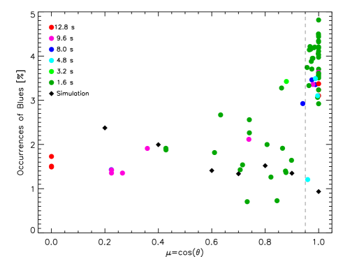
Figure 10.— Fractional number of the occurrences of blue-only profiles with respect to pixels that have a Stokes-V signal greater than $4\sigma$ and their location on the solar disk. The vertical dashed line delimits the population I (right) and II (left) (see Appendix). The color code stands the exposure time of the observations (see the legend in the plot). Both observations and numerical simulations (diamonds) show a decreasing of blue-only profiles as closer they are to the limb (smaller $\mu$).

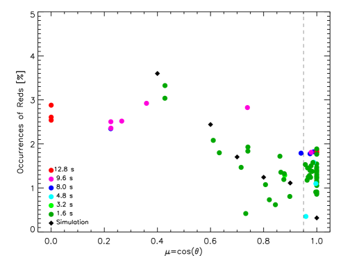
Figure 11.— Number of the occurrences of red-only profiles, following the same symbols as Figure 10.

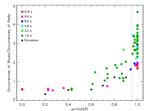
Figure 12.— Ratio between the number of occurrences of blue-only and and red-only profiles as a function of the heliocentric angle. The symbols are the same as in Figures. 10 and 11.

7. Temporal Evolution

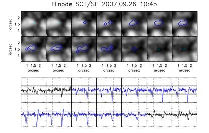
Figure 13.— Top: Example of temporal evolution of blue-only profiles. (from left to right and from top to bottom). Bottom: The most intense blue-only profiles is displayed in blue, while the black line profiles correspond to the location marked with blue light cross before the appearance and after the disappearance of the blue patch. The dashed horizontal lines represent $\pm 5\times 10^{-3}I_{c}$ and $\pm 7\times 10^{-3}I_{c}$ respectively (i.e., $\pm 3\sigma$ and $\pm 4\sigma$). The vertical dashed lines mark the central position of Fe I 6301 Å and 6302 Å.

We have chosen a raster scan of a quiet sun area to show how the patches of single-lobed Stokes V profiles evolve in time. The observation was taken on September, 26 2007 at 10:45 UT, with a spatial sampling of 0.15″ and 0.16″ in X and Y direction, a spectral sampling of 21 $m$Å and an exposure time of 1.6 s. The scan covered an area about 2.7” wide at a cadence of 35 s. Figure 13 shows the temporal evolution of a small area during 8.2 minutes (14 consecutive raster scans).

The temporal evolution of a granule is well centered in the FOV. Although we are interested in the evolution of the blue-only profiles that appear in the second and the third panels, we show some previous and later instants for this small area, too. The blue light crosses mark the positions where the blue-only profiles could be before and after they are observed. The third image of the top row of Figure 13 shows that the blue patch appears at the right part the granule, becoming larger and larger in the next images. Then, it splits in smaller patches, but with the blue-only profiles keeping always concentrated in the right part of the granule. Finally, the blue patch disappears in a large-sized intergranular lane.

The bottom panel of Figure 13 shows the temporal evolution of the observed circular polarization signals. The profiles displayed in blue are the stronger blue-only profiles in the blue patch, while the ones in black are the profiles corresponding to the manually selected positions (blue light crosses in the top panel of Figure 13). As in previous plots, the horizontal dashed lines mark $\pm 3\sigma$ and $\pm 4\sigma$, that roughly correspond to $\pm 5\times 10^{-3}I_{c}$ and $\pm 7\times 10^{-3}I_{c}$ respectively. The vertical dashed lines mark the center of the Fe I 6301 Å and 6302 Å spectral lines. The single-lobed Stokes V profiles appear after the granule is formed, and the strength of the signal and size of the patch increases with time until the granule starts to disappear. From the available time-series, before of the images shown in the plot, the profiles in this area are noisy and start to show a single lobe (similar to the first profile displayed in Figure 13). At these instants, note that the Stokes V signal of Fe I 6301 Å is negligible. Later, this weak signal increases until the first proper blue-only profile appears. At the end, the Stokes V profiles are weak but show regular shapes with two opposite sign. These signals persist during several minutes after the disappearance of the single-lobed profiles, as can be seen in Figure 13.

To better illustrate this, Figures 14 and 15 show the spatial distribution of the Stokes V profiles in the first and last images of the sequence respectively (Figure 13). At positions (4,4) and (5,4) of Figure 14, we can see very tiny single-lobed Stokes V profiles and, in their surroundings, at (2,2) and (3,2), a few asymmetric profiles with very small signal, or noisy profiles. In Figure 15, around position (4,4), there are also a few profiles with strong asymmetry, although they are not single-lobed profiles. For all the time series of this example no linear polarization signal is detected. Similar behavior has been observed in other scans in the sense of the evolution of the blue-only profile amplitude and the size of the blue-only patch. The disappearance of the blue-only profile and any signal in Stokes V evolve together with the granule, i.e., both structures, the granule and the Stokes V signal decrease and collapse.

The evolution shown in Figure 13 suggest a failure of emergence of a tiny magnetic structure which at the end of its life is submerging with the disappearance of the granule.

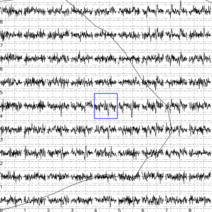
Figure 14.— Spatial distribution of the Stokes V profiles around the blue light cross of the first image of the first row of Figure 13. The profile corresponding to this position is enclosed in the blue light frame. The dashed lines correspond to $\pm 5\times 10^{-3}I_{c}$ and $\pm 7\times 10^{-3}I_{c}$ (i.e., $\pm 3\sigma$ and $\pm 4\sigma$). The overlapped black line displays the intensity contour of the granule.

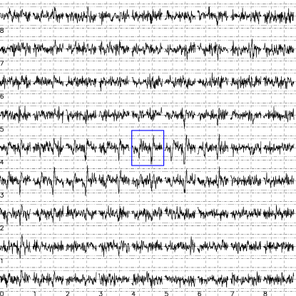
Figure 15.— Similar to Figure 14, but for the position marked with a blue light cross in the last image of the second row of Figure 13. This position is located in a large intergranuliar lane, far away of the granule border.

Figure 16.— Top: example of temporal evolution of red-only profiles. (from left to right and from top to bottom). The lapse between images is 35 s. Three steps before and after of the detected red-only profiles are shown and marked with red crosses. Bottom: in black, the Stokes V profiles corresponding to the red crosses. In red, the red-only profiles.

The size of the red-only patches is of the order of the spatial resolution of Hinode, and their lifetime (few minutes) is considerable shorter than of the blue-only profiles. Figure 16 shows an example of evolution of red-only profiles. They were observed on September, 26 2007 at 08:15 UT. The red patches are mainly located in the intergranular lane, a very changing and dynamic region. The amplitude in Stokes V varies in small spatial scales along the intergranular lane. There are three steps before and after (detection) of the red patch. At the beginning, it is located inside of an irregular-shaped interganular lane, becoming well-defined shape as the granules around appear. The patch size seems to be constrained to the size of the intergranular lane. In the bottom of Figure 16 is plotted the evolution of the profiles. The ones in black correspond to instants before and after the code detects the presence of only one lobe. The profile evolution starts with a small single-lobed Stokes V profiles - below $\pm 3\sigma$ level - increasing the signal as the patch is becoming larger. The amplitude of the single lobe profile increase with the size of the red patch. When it reaches the largest size, it occupies roughly half of the intergranular lane (3^rd image in the 2^nd row of Figure 16). Afterwards, it decreases in area and amplitude until the single lobe has small signal and the code does not detect it. For a large period of time, there are regular Stokes V profiles next to the weak single lobed profile.

Figures 17 and 18 show the spatial distribution of the Stokes V profiles around the positions marked by the first and last red cross of Figure 16. The profiles show in Figure 16 are located at [4,4] in the two cases. At the beginning of the evolution (see Figure 17) there is an area located in the left upper part of the panel where the profiles have rather symmetric Stokes V profiles. In this region, the intensity images (see top panel of Figure 16) show an emergence or rise of a small granule (left top to the cross) and expansion of the big granule (left to the cross). However, in the region where the red patch will appear, there are some small red-only profiles, that becomes red-only profiles (i.e., detected by the code) three images later. Similarly, at the final stage of the evolution (see Figure 18), there are some symmetric Stokes V profile to the right of the selected profile. These symmetric profiles become stronger with time as the granule occupy the intergranular lane, while the signal of the red-only profiles (and the profiles located to the left) drops below $3\sigma$. The red-only profiles do not show significant linear polarization signal during their evolution. Very weak linear signals can however be seen in the surrounding pixels with symmetric Stokes V profiles, as mentioned. In summary, the red-only profiles are well located in the intergranular lane during their life, even when they are surrounded by symmetric Stokes V profiles. Some red-only profiles can possibly appear in the outer part of granules. In this case they do in very small, isolated patches. We have verified that these red isolated patches are related with locations where there were bigger red patches previously, and they have eventually been occupied by the expanding outer part of the granule.

Figure 17.— Spatial distribution of the Stokes V profiles around the red cross of the first image of the first row of Figure 16. The profile corresponding to this position is enclosed in the red frame. The dashed lines correspond to $\pm 5\times 10^{-3}I_{c}$ and $\pm 7\times 10^{-3}I_{c}$ (i.e., $\pm 3\sigma$ and $\pm 4\sigma$). The overlapped black line displays the intensity contour of the granule.

Figure 18.— Similar to Figure 17, but for the last position in Figure 16.

8. Inversions

We have used the SIRJUMP code to invert the observed Stokes profiles. Based on SIRGAUSS (Bellot Rubio, 2003), this code can handle discontinuities or jumps in all the atmospheric parameters or some of them. The discontinuities are located at the same optical depth for the selected parameters. Initially, the amplitudes of the jumps are provided by the user, and then modified by the code until the differences between the observed and synthetic profiles are minimized. Examples of the application of this code to Hinode spectropolarimetric measurements can be found in Louis et al. (2009).

In this paper, we show that one-component model atmospheres with discontinuities of $|{\mathbf{B}}|$ and the line-of-sight velocity ($v_{LOS}$) can explain the observed blue-only and red-only profiles. To that end, we have inverted the profiles displayed in Figure 1 using a fixed magnetic filling factor of 1, i.e., assuming that the whole pixel is occupied by the same atmosphere showing discontinuous stratifications. These profiles come from the two positions marked with yellow crosses in Figure 2. The colored dotted line in Figure 1 displays the best-fit profiles returned by SIRJUMP. Figures 19 and 20 show the temperature, $v_{LOS}$, the strength and the inclination of the magnetic field that the inversion code gave as solution. For simplicity, we only show here the observed and best fit Stokes I and V, although the inversion was done taking into account the four Stokes parameters as one can see in Figure 1. The vertical dashed lines delimit the region $-2<\log(\tau)<0$, where Fe I 6301 Å and 6302 Å  are more sensitive to perturbations of the atmospheric parameters (Ruiz Cobo & del Toro Iniesta, 1992, 1994).

For the blue-only profiles (Figure 19) we retrieve a sharp discontinuity around $\log(\tau)=-0.7$. Below the discontinuity, the magnetic field has a strength of some 270 G and is rather inclined, making 120^∘ to the vertical. In the same layers, we observe upflows of 2.5 km $s^{-1}$. Above the discontinuity, both the magnetic field strength and the LOS velocity are reduced significantly, down to 150 G and 0 km $s^{-1}$. With an inclination of 89^∘, the magnetic field becomes more horizontal and even changes polarity. The configuration deduced from the inversion of the full Stokes vector showing blue-only profiles corresponds to a relatively weak magnetic field which is ascending in the deep layers toward a nearly field-free region at rest in higher layers.

For the red-only profile  shown in Figure 20, the variation of these physical magnitudes occurs basically in the region $-1.2<\log(\tau)<-0.8$. In this region, the velocity changes by 1.9 km s^-1 and the strength and inclination of the vector field by roughly 95 G and 31^∘, respectively. In other words, in the lower part of the atmosphere there exists a magnetized atmosphere with a strong downflow, while in the upper part the atmosphere contains unmagnetized plasma flowing upwards.

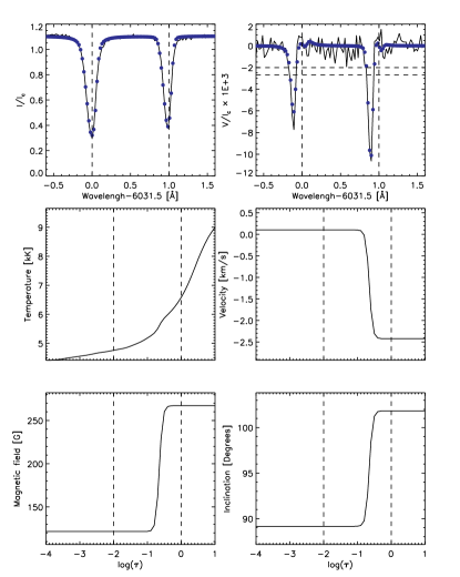
Figure 19.— SIRJUMP inversion of blue-only profiles. Top: observed and best-fit Stokes I and V profiles (solid line and blue dotted line, respectively). The observed profiles are those displayed in Figure 2 (the four Stokes profiles are shown in Figure 1). Mid and bottom: temperature, velocity, magnetic field strength and inclination retrieved from the inversion. Negative velocities indicate upflows. As can be seen, all the atmospheric parameters show discontinuous stratifications within the line formation region.

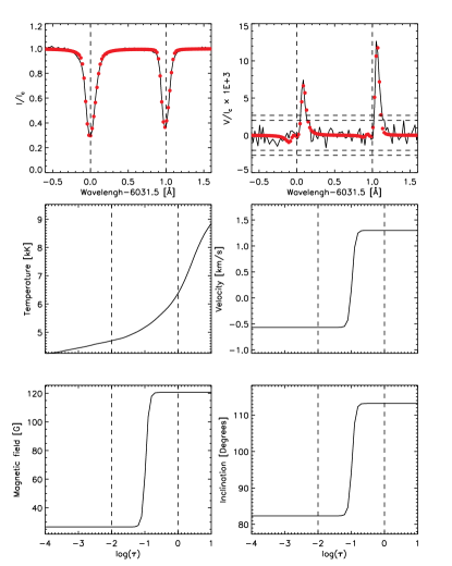
Figure 20.— Same as Figure 19, for the red-only profiledisplayed in Figure 2.

The good fits provided by SIRJUMP demonstrate that the single lobed Stokes V profiles can be explained with discontinuities in some atmospheric parameters. Both inversions show a stronger magnetic field in the lower layers than in the higher layers and rather inclined field lines in the lower part of the atmosphere. Note that the strong field is emerging (submerging) for the blue-only profile (red-only profile). This suggests that some of these profiles might be related to the local evolution of the magnetic field within the granule.

9. Numerical simulation

To gain a better understanding of the physical mechanisms behind the single-lobed Stokes V profiles and complement the inversions, we synthesized Stokes profiles in Fe I 6301 Å and 6302 Å from realistic 3D radiative MHD simulations of flux emergence. The simulations were run with the Bifrost code, which solves the MHD equations with radiative transfer and conduction along the magnetic field (Gudiksen et al., 2011). The synthetic profiles were calculated a posteriori using the SIR code and the modeled atmospheres resulting from the simulation.

The computational domain stretches from the upper convection zone (1.4 Mm below the photosphere) to the lower corona. We use a non-uniform grid of $512\times 256\times 325$ points spanning $16\times 8\times 16$ Mm³, which implies a horizontal grid spacing of $32$ km. The frame of reference for the model is chosen so that $x$ and $y$ are the horizontal directions. The grid is non-uniform in the $z$-direction to ensure that the vertical resolution is good enough to resolve the photosphere and the transition region with a grid spacing of $28$ km, while becoming larger at coronal heights where gradients are smaller.

The initial model is seeded with magnetic field, which rapidly receives sufficient stress from photospheric motions to maintain coronal temperatures ($T>500\,000$ K) in the upper part of the computational domain, as first accomplished by Gudiksen & Nordlund (2004). In the photosphere, the unsigned initial magnetic field has a strength of $160$ G and is distributed in two “bands” of vertical field centered around roughly $x=7$ Mm and $x=13$ Mm. As a result, the magnetic field lines expand into the corona forming loops oriented roughly along the $x$-axis.

To simulate the emergence of magnetic flux, we introduced a non-twisted flux tube into and through the lower boundary of the model. Specifically, horizontal fields of strength $10^{3}$ G were injected in a band of 1.5 Mm wide parallel to the $y$-axis and centered at $x=8$ Mm through the bottom boundary, 1.4 Mm below the photosphere (for details, see the simulation labeled B1 in Martínez-Sykora et al., 2009). Hence, the injected magnetic field is nearly perpendicular to the orientation of the pre-existing ambient field outlined by the coronal loops. This configuration is meant to provide a rough representation of actual conditions in the quiet sun, where flux is emerging continually into a preexisting magnetic field.

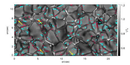
Figure 21.— Synthetic intensity map is shown at the photosphere in grey scale. Blue-only and red-only profiles locations are overplotted with blue and red patches respectively.

To compute synthetic Stokes profiles we considered each column of the simulation as an independent one-dimensional atmosphere. The physical parameters were interpolated to an evenly-spaced logarithmic optical depth grid with stepsize $d\log\tau=0.03$. To identify single-lobed Stokes V profiles we applied the code described in section 3 to the synthetic profiles with $\sigma=8\times 10^{-4}I_{c}$. We did not degrade the synthetic profiles to the spatial or temporal resolution of Hinode. However, the profiles were convolved with the spectral PSF and resampled to the Hinode wavelength scale. We have also synthesized the Stokes profiles for different $\mu$ values: 1.0, 0.9, 0.8, 0.7, 0.6, 0.4 and 0.2. That is, we have considered rays passing through the simulated models with an inclination to the vertical of roughly $0^{\circ},\ 26^{\circ},\ 37^{\circ},\ 46^{\circ},\ 53^{\circ}$ and 78^∘.

The simulation shows many examples of blue-only and red-only profiles (see blue and red patches in Figure 21). In agreement with the observations, the red-only profiles are mostly located in the intergranular lanes and the blue-only profiles are mostly centered in the outer part of the granules, although the patches are slightly smaller than the observed ones.

The fraction of single-lobed profiles as a function of heliocentric angle is presented in Figures 10, 11 and 12 with black diamonds. As can be seen, the red-only and blue-only profiles are slightly less frequent than in the observations. This could be due to several reasons: i) we did not degrade the profiles to the Hinode spatial and temporal resolution; ii) the vertical spatial resolution of the model may be not good enough to produce sharp jumps in the photosphere; iii) the magnetic field configuration might be too simplistic; iv) the amount of magnetic flux emergence in the box is probably different from that occurring in the quiet sun. However, the ratio of the blue-only to the red-only profiles seems to agree with the observations (Figure 12). Moreover, the trend of the number of the occurrences of blue-only profiles with $\mu$ is very similar to the observations (Figure 10). For the red-only profiles, the number of occurrences increases with $\mu$, and for $\mu<0.6$ it remains almost constant (Figure 11).

In the simulations, we see that many different stratifications produce single-lobed Stokes V spectra. These stratifications are often complex because of the chaotic structure of the magnetic field in the photosphere. However, most of them can be categorized in two broad classes which show discontinuities or strong variations of the physical parameters with height. The first group includes atmospheres where the magnetic field is mostly concentrated in the deep layers. The second group is that of canopy-like structures, i.e., a magnetized region on top of a nearly-field free plasma. Hereafter we will call them “deep-field” and “high-field” configurations, respectively.

An example of the typical deep-field configuration for blue-only profiles is given in Figure 22. At the location of the selected profile, the atmosphere exhibits a discontinuity with a rather large jump in the magnetic field strength similar to that obtained from the inversions. The field in deep layers is much stronger than the ambient field above ($\sim$300 G vs $\sim$30 G). The velocity shows a strong gradient instead of a jump, with large upflows in the deep layers and nearly zero velocities in the high layers. The magnetic field inclination varies only slightly. This configuration, which is very similar to that inferred from the inversion, is produced by a small-size magnetic $\Omega$ loop emerging at the edge of a granule. The magnetic topology around the location of the blue-only profile is shown in the bottom panel of Figure 22. As can be seen, the magnetic field in deep layers is stronger (purple in the figure) than the ambient field above (yellowish) and exhibits upflows. The $\Omega$-loop is strongly bent at the photosphere and only one of its footpoints is located inside the granule. As is usually the case, this blue-only profile is located at the edge of the granule but not yet in the intergranular lane. It lasts for about 11 minutes.

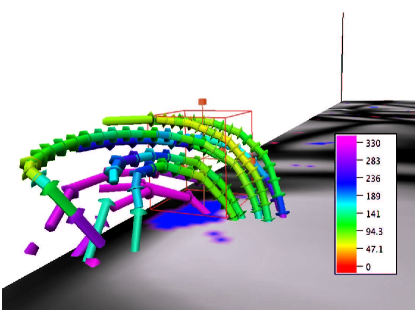
Figure 22.— Blue-only profile observed in the simulation at $[x,y]=[12.6,0.2]$ arcsec and the associated deep-field configuration producing it. The layout of the three first rows is the same as in Figure 19. The synthetic spectra have been convolved with the spectral PSF of Hinode and sampled with a wavelength step of 21.5 $m$Å. The horizontal dashed lines in the top-right panel are drawn at the $\pm 3\sigma$ and $\pm 4\sigma$ levels. The bottom panel displays a 3D view of the MHD model. The magnetic field is shown with vectors where the color scheme represents the magnetic field strength. The background image in grey is a continuum intensity map. The red box indicates the optical depth range $-2<\log(\tau)<0$ for the pixel showing the blue-only Stokes V profile. The blue and red patches mark the location of red-only and blue-only profiles.

Blue-only profiles can also be produced by high-field (canopy-like) configurations with upflows in the deep layers. In the example of Figure 23, the lower part of the photosphere has nearly zero magnetic fields ($\sim$80 G) and strong upward velocities ($\sim$-3 km s^-1). Higher layers show stronger fields ($\sim$160 G) and nearly zero velocities ($\sim$-0.5 km s^-1). Only the magnetic field strength and inclination show abrupt jumps. The velocity also varies quite strongly with depth, but in a more linear fashion. Note that the gradient of magnetic field strength and cosine of the field inclination have opposite signs. In this case, it is the variation of the inclination that determines the sign of the area asymmetry (i.e., the suppression of the Stokes V red lobe), because the magnetic field is nearly horizontal. In fact, most of the high-field configurations for the blue-only profiles show this type of stratification. Interestingly, the field strength attains a minimum in the mid-photosphere, which suggests an interaction between two flux systems— possibly a reconnection process. As can be seen in the 3D view at the bottom of Figure 23, the group of field lines in the lower part of the volume has the shape of a small $\Omega$-loop. The stronger magnetic field above is connected to other magnetic structures further away. Looking at the time evolution we observe that the upper field lines emerge and expand into the chromosphere. The duration of this profile is also 11 minutes.

Figure 23.— Example of a blue-only profile produced by a high-field (canopy-like) configuration at $[x,y]=[4.9,7.7]$ arcsec. The different panels are arranged as in Figure 22.

In the simulations, $\sim$85% of the observed blue-only profiles are due to deep-field configurations associated with magnetic flux emergence at the border of granules. About 65% of the blue-only profiles show a discontinuous magnetic field strength stratification like in Figure 22, while $\sim$20% exhibit a strong field strength gradient instead of a pure discontinuity. The jump of the different parameters is mostly located deep in the photosphere, inside the optical depth range $-1<\log(\tau)<0$. A velocity gradient of the type shown in Figure 22 is present in most of the blue-only profiles ($\sim$95%).

Another $\sim$10% of the blue-only profiles are associated with high-field, canopy-like configurations similar to that shown in Figure 23 (note the complexity of the magnetic field). The vast majority (99%) of the high-field configuration exhibits a discontinuity in the magnetic field strength. These discontinuities are usually located above $\log(\tau)=-1$.

Finally, the remaining 5% of blue-only profiles are the result of complex atmospheric stratifications which do not fit in these two classes. Irrespective of their origin, all the blue-only profiles show large upflows in deep photospheric layers and nearly zero velocities higher up.

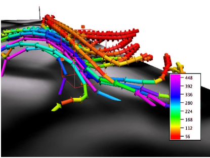
Figure 24.— Example of a red-only profile arising from a deep-field configuration at the location $[x,y]=[5.5,1.1]$ arcsec. The arrangement of the panels is as in Figure 22.

We find that also the red-only profiles are produced by deep-field and high field configurations, this time associated with downflows. The most common source of red-only profiles is the deep-field configuration, a typical example is shown in Figure 24. This atmosphere exhibits a discontinuity in magnetic field, which is much stronger in deep layers ($\sim$400 G vs 100 G). The velocity shows a strong gradient with large downflows in the deep layers ($\sim$5 km s^-1 vs 0.5 km s^-1). The field inclination has a small jump from slightly inclined field in the lower layers to horizontal field in the higher layers. This configuration is in agreement with the stratification obtained from the inversion of the red-only profiles of Figure 1. The rather strong and deep magnetic field is confined along the intergranular lane almost parallel to the photosphere as shown in Figure 24. These lines end into the photosphere as an $\Omega$-loop. Above them, another set of field lines, also following the path of the intergranular lane, have weaker magnetic strength and are connected to a different place in the photosphere. The deep magnetic field is submerging into the intergranular lane. The duration of this red-only profile is roughly 12 minutes.

Figure 25.— Red-only profile due to a high-field configuration at $[x,y]=[1.9,6.7]$ arcsec. The arrangement of the panels is as in Fig 22.

An example of a high-field configuration leading to red-only profiles is displayed in Figure 25. For these profiles to appear it is necessary that the deep photosphere has weaker magnetic field and stronger upward velocities than the high photosphere ($\sim 5$ G vs 80 G and $\sim$ -3.5 vs -0.4 km s^-1, respectively). The magnetic field strength and inclination show a rather strong jump, while the LOS velocity exhibit a steep gradient. This configuration is a clear example of a canopy atmosphere. Note that this particular red-only profile is located inside the granule as shown in the 3D image in the bottom panel of Figure 25. The group of field lines located in the lower photosphere has the shape of a tiny $\Omega$-loop. These tiny loops show a strong turn over at the height where the strong magnetic fields are located higher up. The lifetime of this profile is roughly four minutes, because the “canopy” appears only during the splitting in two parts.

In summary, in the simulation most of the red-only profiles (82%) are associated with magnetic fields that are submerging (as the example shown in Figure 24). About $\sim$70% of them have a discontinuity in the magnetic field strength and $\sim$15% show a smooth decrease of the magnetic field strength with height. Sometimes, the field strength reaches a minimum in between the ambient and the submerging field, which suggests an interaction between the two flux systems, possibly a reconnection process (20% of the cases). About $\sim$15% of the red-only profiles are produced by a high-field configuration such as that of the Figure 25. Finally, the remaining 2% of red-only profiles are the result of complex atmospheric stratifications which do not fit in these two classes.

Thus, the stratifications that lead to single-lobed Stokes V profiles in the simulations support the main conclusion derived from the inversion, namely that jumps in the physical parameters along the line of sight can explain the existence of single lobed profiles. This is not the only mechanism capable of producing such anomalous signals, since other types of stratifications also generate circular polarization profiles with only one lobe, but it is the most common as observed in the simulations.

From the many stratifications producing the single-lobed profiles in the simulations, when the stratification is simple enough, we note that if the variation of the velocity with height is opposite (equal) to the variation of the magnetic field strength with height, the single-lobed Stokes V is blue-only (red-only) in accordance with the rules deduced by Solanki & Pahlke (1988) and Steiner (1999). This is not the case for the example of Figure 23 because in that case the important parameter is the gradient of the cosine of the magnetic field inclination.

10. Summary

Using Hinode spectropolarimetric measurements, we have performed an in-depth characterization of the circular polarization profiles with only one lobe observed in the quiet sun network and internetwork. We have successfully inverted them in terms of model atmospheres featuring discontinuities in the parameters along the line of sight. The scenario indicated by the inversions is supported by the results of 3D MHD simulation which also show an abundance of blue-only and red-only Stokes V profiles.

The main properties of these profiles can be summarized as follows:

• The blue-only profiles are mainly located in the outer part of the granules, therefore they are more often related with upflows. They form patches as large as $1\arcsec\times 1\arcsec$ and their mean lifetime is slightly shorter than the granule lifetime.

• The red-only profiles are mainly located in the intergranular lanes, therefore they are more often related with downflows. They tend to form very small structures, sometimes as small as a single pixel, i.e., $0.15\arcsec\times 0.16\arcsec$.

• The ratio of blue-only to red-only profiles drastically decreases from the center to the limb of the solar disk. This variation can be traced back to a strong reduction of the number of blue-only profiles. Such a reduction may be caused by the upward shift of the $\tau=1$ level toward the limb, which makes it difficult or even impossible to reach the deep layers where these “granular” profiles are formed.

• The area occupied by the single-lobed Stokes V profiles on the solar surface is less than 2% ($\sim$1% of the area is occupied by blue-only profiles and $\sim$0.4% by red-only profiles).

• However, the fraction of blue-only and red-only profiles, compared to the profiles that show clear signal in Stokes V, are 4% and 1%, respectively.

• The single-lobed Stokes V profiles are located in the surroundings of network patches, never inside them. They are often located in places where there are simultaneously both circular and linear polarization signals, which suggests that they are associated with inclined fields, or that they occur because of a sudden change in the direction of the magnetic field.

• Both the blue-only and red-only profiles show weak or modest circular polarization signals and weak linear polarization signals.

• The evolution of the single-lobed Stokes V profiles is related to the evolution of the granules and intergranular lanes that host them.

• Inversion of the four Stokes profiles based on models featuring discontinuities along the LOS can reproduce the observed single-lobed Stokes V profiles.

• Synthetic single-lobed profiles are observed in realistic 3D numerical simulations. Several types of stratifications can explain these profiles, but most of them show discontinuities in at least one of the parameters (usually the magnetic field strength or the inclination) as was inferred from the inversion. A large fraction of these stratifications show a strong velocity gradient instead of a jump.

• The number of single-lobed profiles and the statistics from the simulations are quiet similar to the observations, but there exist small differences that might be caused by missing physics (see Section 11).

11. Discussion and Conclusions

The statistical and physical properties of the single-lobed Stokes V profiles tell us that they cannot be explained as the superposition of opposite-polarity Stokes V profiles or as unusual events on the solar surface. On the contrary, they show clear features associated with physical processes that could involve a sharp or drastic change of the orientation and strength of the magnetic field occurring mainly between the outer part of granules and the adjacent intergranular lanes.

From the few temporal evolutions that we studied, the blue-only profiles suggest a magnetic flux emergence processes, with lifetime comparable to the granulation lifetime. Therefore, these patches first appear with weak polarization signal, then increase in size and strength. Finally, the blue-only patches disappear, but small Stokes V signal remain in the region where the blue-only patches were sited for roughly one minute. We do not detect linear polarization with this profiles At the end, the signal in Stokes V disappears with the disappearance of the granule, perhaps as result of a submergence process.

We used the SIRJUMP inversion code on this study after selecting suitable cases. This code can handle strong variations of the vector magnetic field and velocity along the line of sight, i.e., it can model a magnetopause or slab structure in the pixel. In fact, both the inversion and the numerical simulations indicate that single-lobed profiles can be produced by discontinuities along the line of sight. In the simulations a wide range of atmosphere give rise to Stokes V profiles with only one lobe. However, most of them are related to emerging magnetic field (blue-only) and disappearing or submerging magnetic field (red-only). Therefore, the statistical comparison between observations and simulations provides a tool to determine both the magnetic field topology in the quiet sun and its emerging and disappearing process in the local granulation. The lifetime of the single-lobed Stokes V profile must tell us the duration of the emergence and the submergence, i.e., the duration of the fundamental input and output processes of magnetic flux.

The absence of blue-only profiles near the limb might be due to these small structures being located in the lower-middle atmosphere while the red-only profiles might be located more or less equally at different heights or with some preference higher layers (this is supported by what we observed in the inversions and in the forward model).

As mentioned above, the simulation has a small discrepancy with the observations in the statistics. This discrepancy could be due to the following reasons:

• The vertical spatial resolution of the simulations is not good enough.

• The spatial resolution of Hinode was not taken into account.

• The amount of mean magnetic field, or the simplified initial magnetic configuration, may be off.

• It is probably necessary to input periodically a specific amount of new emerging magnetic flux in the simulation. The input of new flux might require a different type of magnetic field configuration in the bottom boundary. Moreover, the duration of each patch with new flux should last as long as the mean lifetime of the blue-only profiles (as shown in Section 7).

Once the simulations have good grid resolution and the synthetic profiles have been convolved with the spatial and spectral PSF, then any remaining discrepancies between observations and simulations must tell us with which frequency, where, and how long new and small structures of magnetic field have to be injected. In order to approach a realistic simulation of the convection zone and photosphere of the quiet sun, the simulations must to reproduce the statistic study presented here (Sections 4-6).

We have focussed our attention on the quiet sun, but plage, active regions, and ephemeral regions might behave differently. Thus, it is important to carry out similar studies in those structures for a better understanding of their magnetic topology and evolution.

12. Acknowledgments

This work was partially carried out while ASD was a Visiting Scientist at the Instituto de Astrofísica de Andalucía. Financial support by the Spanish MICCIN through projects AYA2009-14105-C06-06 and PCI2006-A7-0624, and by Junta de Andalucía through project P07-TEP-2687 (including a percentage from European FEDER funds) is gratefully acknowledged. Part of the data used here were acquired in the framework of HOP 14 (Hinode-Canary Islands joint campaign). Hinode is a Japanese mission developed by ISAS/JAXA, with NAOJ as domestic partner and NASA and STFC (UK) as international partners. It is operated in cooperation with ESA and NSC (Norway). The Hinode project at Stanford and Lockheed is supported by NASA contract NNM07AA01C (MSFC). ASD thanks the International Space Science Institute (hereafter ISSI) and I. Kitiashvili for the invitation to participate in the meeting ‘Filamentary Structure and Dynamics of Solar Magnetic Fields,’ 15-19 November 2010, ISSI, Bern, where many aspects of this paper were discussed with other colleagues. This work has also benefited from discussions in the Flux Emergence meetings held at ISSI, Bern in February and December 2011. We thank T. Tarbell for his corrections and suggestions. The 3D simulations have been run with the Njord and Stallo cluster from the Notur project and the Pleiades cluster through computing grants SMD-07-0434, SMD-08-0743, SMD-09-1128, SMD-09-1336, SMD-10-1622, SMD-10-1869, SMD-11-2312, and SMD-11-2752 from the High End Computing (HEC) division of NASA. We thankfully acknowledge the computer and supercomputer resources of the Research Council of Norway through grant 170935/V30 and through grants of computing time from the Programme for Supercomputing. To analyze the data we have used IDL and Vapor (http://www.vapor.ucar.edu).

The first seven columns in Table LABEL:latabla show parameters for all the observation runs. The spectral sampling was 21.5$\pm$0.1 $m$Å for all of them.

Figure 26 shows the spatial distribution of the studied observational runs: the data pool. In the plane XY is drawn the solar disk (both axis are given in arcsec). The drawing pins locate the position of the selected 72 Hinode SOT/SP observation run. The length of drawing pins represents the exposure time of the observation. In addition, we have used different colors for each exposure time.

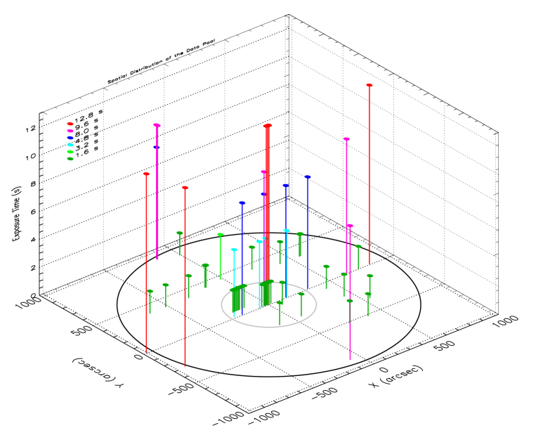
Figure 26.— Distribution of the data pool on the solar disk. In the inner grey circle are 61% of the studied observation runs, that we have called population I. They were observed with a wide range of exposure time. Out of this inner grey circle stays the population II. They were mainly observed with long time exposure time.

We have selected 72 observation runs with different exposure time. 61% of the observations are located at $1.00<\mu<0.95$, which are inside of the inner grey circle (see Figure 26). The observation runs inside the inner circle have a wide range of exposure times (1.6, 4.8, 8.0 9.6 and 12.8 s). For understanding the possible influence of the projection effect in the behavior of the single-lobed Stokes V profiles we have selected observations out of this centered region of the solar disk and in the limb (even two observation scans started very off the limb but ended inside the solar disk). Therefore, we can talk about two populations or sets in our data pool: one is inside the inner circle (with a low influence of projection effect), hereafter called as population I, and the other is outside of this inner circle (with not negligible projection effect), which is referred as population II.

Most of the scans were taken in quiet sun, both large area scans and temporal scans. We have also selected a few temporal scans taken over a part of sunspot or pore, but always including the photospheric network in their field of view. In addition, several scans close to the limb include points off the solar disk. These three kind of maps have been indicated in the last column of Table LABEL:latabla labeled SS, P and OL that stand for sunspot, pore and off the limb observations respectively.

Table 1Data Pool. From left to right: date and time, spatial scales, position on the solar disk, exposure time and signal to noise ratio, percentage of blue-only profiles, and red-only profiles, the rate between them, and a description the observations: temporal scan (TS, with the strip width expressed in granules), large scan (LS), sunspot (SS), pore (P) and off the limb (OL).

Date Time	X scale	Y scale	( X, Y)	$\mu$	Exp. Time	S/N	B	R	B/R	Desc.
	(″)	(″)	(″, ″)		(s)		(%)	(%)
2007.02.19 21:31	0.30	0.32	( -4.3, 7.6)	1.000	1.6	1189	3.7	1.4	2.7	TS (1)
2007.02.24 02:28	0.30	0.32	( 415.5, -70.3)	0.899	1.6	1148	1.6	0.8	2.0	TS (5)
2007.02.27 11:51	0.15	0.16	(-271.2, 18.7)	0.959	4.8	631	1.2	0.4	3.4	TS (5) & SS
2007.09.01 20:35	0.15	0.16	(-153.1, 922.9)	0.224	8.0	549	1.4	2.3	0.6	LS
2007.09.06 00:28	0.15	0.16	(-153.1, 922.8)	0.225	9.6	630	1.4	2.4	0.6	LS
2007.09.06 13:11	0.15	0.16	(-214.5, 7.0)	0.975	8.0	1146	3.5	1.8	1.9	LS
2007.09.06 15:55	0.15	0.16	( -34.6, 7.0)	0.999	8.0	1150	3.6	1.8	1.9	LS
2007.09.07 11:44	0.15	0.16	( 145.4, 6.8)	0.988	8.0	1138	3.4	1.8	1.8	LS
2007.09.07 15:04	0.15	0.16	( 325.3, 6.8)	0.941	8.0	1110	2.9	1.8	1.6	LS
2007.09.09 07:05	0.15	0.16	( 646.8, 7.2)	0.739	9.6	957	2.1	2.8	0.7	LS
2007.09.09 13:05	0.15	0.16	( -79.0,-892.6)	0.359	9.6	868	1.9	2.9	0.7	LS
2007.09.10 01:15	0.15	0.16	(-153.1, 922.9)	0.225	9.6	634	1.4	2.5	0.5	LS
2007.09.10 08:00	0.15	0.16	( -34.2, 6.8)	0.999	9.6	1275	3.6	1.8	2.0	LS
2007.09.11 06:10	0.15	0.16	(-935.5,-291.0)	0.000	12.8	950	1.7	2.9	0.6	LS
2007.09.11 14:06	0.15	0.16	(-153.1, 912.7)	0.266	9.6	682	1.4	2.5	0.5	TS (1)
2007.09.15 12:44	0.15	0.16	( -92.0,-173.1)	0.979	9.6	14438	3.4	1.8	1.8	LS
2007.09.16 07:23	0.15	0.16	( -21.8, 6.5)	1.000	4.8	873	3.6	1.5	2.4	TS (1)
2007.09.19 07:11	0.15	0.16	( -16.6, 456.7)	0.879	3.2	685	3.4	1.3	2.7	TS (2)
2007.09.24 11:56	0.15	0.16	( -6.9, 7.4)	1.000	1.6	544	3.6	0.9	4.0	TS (1)
2007.09.24 19:32	0.15	0.16	( -15.8, 6.7)	1.000	12.8	1461	3.1	1.9	1.7	LS
2007.09.24 20:42	0.15	0.16	( -5.1, 6.7)	1.000	12.8	1489	3.4	1.8	1.9	LS
1007.09.24 21:52	0.15	0.16	( 5.7, 7.0)	1.000	12.8	1464	3.2	1.9	1.7	LS
2007.09.25 12:59	0.15	0.16	( -26.3, 6.5)	1.000	1.6	547	4.5	1.3	3.5	TS (1)
2007.09.26 08:15	0.15	0.16	( -7.7, 6.4)	1.000	1.6	531	3.6	1.1	3.4	TS (1)
2007.09.26 10:45	0.15	0.16	( -4.9, 6.5)	1.000	1.6	547	2.9	0.9	3.3	TS (1)
2007.09.26 18:03	0.15	0.16	( 835.6, 7.6)	0.492	12.8	768	1.5	2.5	0.6	LS
2007.09.27 01:01	0.15	0.16	(-1004., 7.5)	0.000	12.8	887	1.5	2.6	0.6	LS & OF
2007.09.28 07:00	0.15	0.16	( -19.3, 6.4)	1.000	1.6	535	3.2	1.1	2.8	TS (1)
2007.09.29 06:51	0.15	0.16	( -20.7, 6.4)	1.000	1.6	539	4.2	1.3	3.1	TS (1)
2007.10.01 08:21	0.15	0.16	( -6.6, 7.3)	1.000	1.6	535	4.2	1.3	3.2	TS (1)
2007.10.04 10:41	0.30	0.32	( -16.1, 6.5)	1.000	1.6	1169	4.0	1.4	2.9	TS (10)
2007.10.05 08:05	0.30	0.32	( -17.6, 6.5)	1.000	1.6	1139	4.1	1.2	3.4	TS (10)
2007.10.05 11:23	0.30	0.32	( -15.4, 6.3)	1.000	1.6	1167	4.3	1.9	2.3	TS (10)
2007.10.18 19:11	0.30	0.32	( 434.5,-221.7)	0.861	1.6	1085	3.3	1.7	1.9	TS (8)
2007.10.23 05:28	0.30	0.32	(-121.9,-250.4)	0.957	1.6	1141	3.7	1.5	2.4	TS (8)
2007.10.24 01:04	0.30	0.32	( 58.3,-249.5)	0.964	1.6	1147	3.3	1.2	2.8	TS (8) & P
2007.10.25 00:02	0.30	0.32	( 546.6,-342.5)	0.741	1.6	1066	3.6	1.8	1.4	TS (8)
2007.10.26 03:51	0.30	0.32	( -34.6, 6.3)	0.999	1.6	1158	4.5	1.4	3.1	TS (8)
2007.10.26 19:50	0.30	0.32	( -53.3, 6.0)	0.998	1.6	1138	4.1	1.4	3.0	TS (8)
2007.10.27 02:12	0.15	0.16	( 743.1, 5.1)	0.633	1.6	484	2.7	1.8	1.5	TS (2)
2007.10.29 16:09	0.15	0.16	( -25.5, 6.3)	1.000	1.6	539	4.3	1.2	3.7	TS (2)
2007.10.29 17:54	0.15	0.16	( -9.1, 6.4)	1.000	1.6	543	4.8	1.2	3.9	TS (2)
2007.10.29 19:31	0.15	0.16	( 6.1, 6.4)	1.000	1.6	545	3.5	1.1	3.2	TS (2)
2007.10.29 21:08	0.15	0.16	( 21.3, 6.6)	1.000	1.6	545	4.0	0.9	4.6	TS (2)
2008.07.22 14:05	0.30	0.32	( -22.1, 7.5)	1.000	1.6	1135	4.2	1.5	2.7	TS (2)
2008.07.24 15:01	0.30	0.32	( -13.6, 7.8)	1.000	1.6	1136	4.4	1.8	2.5	TS (2)
2008.07.28 14:13	0.30	0.32	( -20.9, 7.6)	1.000	1.6	1136	3.6	1.5	2.4	TS (2)
2008.07.28 15:52	0.30	0.32	( -6.3, 7.6)	1.000	1.6	1134	3.5	1.2	2.8	TS (2)
2008.07.30 14:22	0.30	0.32	( 65.9, -54.0)	0.996	1.6	1135	3.1	0.9	3.4	TS (2)
2008.07.31 14:25	0.30	0.32	( -8.1, 867.5)	0.428	1.6	886	1.9	3.0	0.6	TS (2)
2008.07.31 16:20	0.30	0.32	( -8.1, 867.4)	0.428	1.6	884	1.9	3.3	0.6	TS (2)
2008.12.22 00:00	0.15	0.16	( -79.3, -2.1)	0.997	4.8	843	3.1	1.1	2.8	TS (5)
2008.12.23 00:00	0.15	0.16	( 148.1, -0.1)	0.988	4.8	837	3.5	1.6	2.2	TS (5)
2008.12.25 11:00	0.30	0.32	(-241.2, 67.5)	0.965	1.6	744	4.1	1.5	2.8	LS
2008.12.25 12:00	0.30	0.32	(-231.9, 67.6)	0.968	1.6	752	4.2	1.2	3.4	LS
2008.12.25 13:00	0.30	0.32	(-222.6, 67.8)	0.970	1.6	753	4.1	1.2	3.3	LS
2008.12.25 14:00	0.30	0.32	(-213.2, 67.8)	0.972	1.6	755	3.9	1.3	3.0	LS
2008.12.25 15:00	0.30	0.32	(-203.9, 67.7)	0.975	1.6	751	3.7	1.4	2.7	LS
2008.12.25 16:00	0.30	0.32	(-194.5, 68.2)	0.977	1.6	751	3.9	1.2	3.2	LS
2008.12.25 17:00	0.30	0.32	(-185.1, 68.3)	0.979	1.6	753	3.9	1.5	2.6	LS
2008.12.25 21:01	0.30	0.32	(-147.1, 68.9)	0.986	1.6	749	4.2	1.6	2.7	LS
2008.12.25 22:01	0.30	0.32	(-166.2, 69.0)	0.982	1.6	713	4.2	1.4	3.0	LS
2009.05.28 10:13	0.30	0.32	( 234.0,-516.5)	0.807	1.6	1044	2.0	1.1	1.9	TS (5)
2009.05.29 09:11	0.30	0.32	( 382.8,-519.0)	0.741	1.6	1010	2.3	1.9	1.2	TS (5)
2009.05.31 08:47	0.30	0.32	(-650.7, 393.6)	0.610	1.6	929	1.8	2.1	0.9	TS (5)
2009.06.01 09:25	0.30	0.32	(-520.9, 394.4)	0.733	1.6	939	0.7	0.4	1.7	TS (8) & SS
2009.06.02 10:03	0.30	0.32	(-331.0, 393.9)	0.844	1.6	838	0.7	0.6	1.2	TS (8) & SS
2009.06.03 07:54	0.30	0.32	(-165.1, 432.6)	0.876	1.6	990	1.4	1.2	1.2	TS (5) & P
2009.06.03 09:01	0.30	0.32	(-155.9, 432.6)	0.878	1.6	964	1.4	1.3	1.0	TS (5)
2009.06.05 08:39	0.30	0.32	( 220.0, 428.7)	0.865	1.6	1055	1.9	1.4	1.4	TS (5)
2009.06.06 09:16	0.30	0.32	( 402.9, 370.6)	0.821	1.6	1040	1.3	0.7	1.7	TS (8)
2009.06.07 08:16	0.30	0.32	( 560.4, 368.9)	0.715	1.6	950	1.5	1.5	1.0	TS (8)
2009.06.07 09:54	0.30	0.32	( 570.7, 368.8)	0.706	1.6	993	1.4	1.6	0.9	TS (8)

References

- Auer & Heasley (1978) Auer, L. H., & Heasley, J. N. 1978, A&A, 64, 67
- Bellot Rubio (2003) Bellot Rubio, L. R. 2003, in Astronomical Society of the Pacific Conference Series, Vol. 307, Astronomical Society of the Pacific Conference Series, ed. J. Trujillo-Bueno & J. Sanchez Almeida, 301–+
- Bellot Rubio et al. (2001) Bellot Rubio, L. R., Rodríguez Hidalgo, I., Collados, M., Khomenko, E., & Ruiz Cobo, B. 2001, ApJ, 560, 1010
- del Toro Iniesta (2003) del Toro Iniesta, J. C. 2003, Introduction to Spectropolarimetry, ed. del Toro Iniesta, J. C.
- Fischer et al. (2009) Fischer, C. E., de Wijn, A. G., Centeno, R., Lites, B. W., & Keller, C. U. 2009, A&A, 504, 583
- Grossmann-Doerth et al. (2000) Grossmann-Doerth, U., Schüssler, M., Sigwarth, M., & Steiner, O. 2000, A&A, 357, 351
- Gudiksen et al. (2011) Gudiksen, B. V., Carlsson, M., Hansteen, V. H., Hayek, W., Leenaarts, J., & Martínez-Sykora, J. 2011, A&A, 531, A154+
- Gudiksen & Nordlund (2004) Gudiksen, B. V., & Nordlund, Å. 2004, in IAU Symposium, Vol. 219, Stars as Suns : Activity, Evolution and Planets, ed. A. K. Dupree & A. O. Benz, 488–+
- Illing et al. (1975) Illing, R. M. E., Landman, D. A., & Mickey, D. L. 1975, A&A, 41, 183
- Kosugi et al. (2007) Kosugi, T., Matsuzaki, K., Sakao, T., Shimizu, T., Sone, Y., Tachikawa, S., Hashimoto, T., Minesugi, K., Ohnishi, A., Yamada, T., Tsuneta, S., Hara, H., Ichimoto, K., Suematsu, Y., Shimojo, M., Watanabe, T., Shimada, S., Davis, J. M., Hill, L. D., Owens, J. K., Title, A. M., Culhane, J. L., Harra, L. K., Doschek, G. A., & Golub, L. 2007, Sol. Phys., 243, 3
- Landi Degl’Innocenti (1992) Landi Degl’Innocenti, E. 1992, Magnetic field measurements, ed. Sanchez, F., Collados, M., & Vazquez, M., 71–+
- Landolfi & Landi Degl’Innocenti (1996) Landolfi, M., & Landi Degl’Innocenti, E. 1996, Sol. Phys., 164, 191
- Louis et al. (2009) Louis, R. E., Bellot Rubio, L. R., Mathew, S. K., & Venkatakrishnan, P. 2009, ApJ, 704, L29
- Martínez-Sykora et al. (2009) Martínez-Sykora, J., Hansteen, V., & Carlsson, M. 2009, ApJ, 702, 129
- Narayan & Scharmer (2010) Narayan, G., & Scharmer, G. B. 2010, A&A, 524, A3+
- Rees et al. (1989) Rees, D. E., Durrant, C. J., & Murphy, G. A. 1989, ApJ, 339, 1093
- Ruiz Cobo & del Toro Iniesta (1992) Ruiz Cobo, B., & del Toro Iniesta, J. C. 1992, ApJ, 398, 375
- Ruiz Cobo & del Toro Iniesta (1994) —. 1994, A&A, 283, 129
- Sanchez Almeida et al. (1996) Sanchez Almeida, J., Landi Degl’Innocenti, E., Martinez Pillet, V., & Lites, B. W. 1996, ApJ, 466, 537
- Schlichenmaier et al. (1998) Schlichenmaier, R., Jahn, K., & Schmidt, H. U. 1998, ApJ, 493, L121+
- Sigwarth (2001) Sigwarth, M. 2001, ApJ, 563, 1031
- Sigwarth et al. (1999) Sigwarth, M., Balasubramaniam, K. S., Knölker, M., & Schmidt, W. 1999, A&A, 349, 941
- Solanki & Pahlke (1988) Solanki, S. K., & Pahlke, K. D. 1988, A&A, 201, 143
- Steiner (1999) Steiner, O. 1999, in Astronomical Society of the Pacific Conference Series, Vol. 184, Third Advances in Solar Physics Euroconference: Magnetic Fields and Oscillations, ed. B. Schmieder, A. Hofmann, & J. Staude, 38–54
- Steiner (2000) Steiner, O. 2000, Sol. Phys., 196, 245
- Tsuneta et al. (2008) Tsuneta, S., Ichimoto, K., Katsukawa, Y., Nagata, S., Otsubo, M., Shimizu, T., Suematsu, Y., Nakagiri, M., Noguchi, M., Tarbell, T., Title, A., Shine, R., Rosenberg, W., Hoffmann, C., Jurcevich, B., Kushner, G., Levay, M., Lites, B., Elmore, D., Matsushita, T., Kawaguchi, N., Saito, H., Mikami, I., Hill, L. D., & Owens, J. K. 2008, Sol. Phys., 249, 167
- Viticchié et al. (2011) Viticchié, B., Sánchez Almeida, J., Del Moro, D., & Berrilli, F. 2011, A&A, 526, A60+
- Viticchié & Vitas (2012) Viticchié, B., & Vitas, N. 2012, A&A, submitted