On Parameterized Gallager’s First Bounds for Binary Linear Codes over AWGN Channels

Abstract

In this paper, nested Gallager regions with a single parameter is introduced to exploit Gallager’s first bounding technique (GFBT). We present a necessary and sufficient condition on the optimal parameter. We also present a sufficient condition (with a simple geometrical explanation) under which the optimal parameter does not depend on the signal-to-noise ratio (SNR). With this general framework, three existing upper bounds are revisited, including the tangential bound (TB) of Berlekamp, the sphere bound (SB) of Herzberg and Poltyrev, and the tangential-sphere bound (TSB) of Poltyrev. This paper also reveals that the SB of Herzberg and Poltyrev is equivalent to the SB of Kasami et al., which was rarely cited in literature.

I Introduction

In most scenarios, there do not exist easy ways to compute the exact decoding error probabilities for specific codes and ensembles. Therefore, deriving tight analytical bounds is an important research subject in the field of coding theory and practice. Many previously reported upper bounds [1, 2, 3, 4, 5, 6, 7, 8, 9, 10, 11, 12], as mentioned in [13], are based on Gallager’s first bounding technique (GFBT)

$${\rm Pr}\{E\}\leq{\rm Pr}\{E,\underline{y}\in\mathcal{R}\}+{\rm Pr}\{\underline{y}\notin\mathcal{R}\},$$ (1)

where $E$ denotes the error event, $\underline{y}$ denotes the received signal vector, and $\mathcal{R}$ denotes an arbitrary region around the transmitted signal vector. The first term in the right hand side (RHS) of (1) is usually bounded by the union bound, while the second term in the RHS of  (1) represents the probability of the event that the received vector $\underline{y}$ falls outside the region $\mathcal{R}$, which is considered to be decoded incorrectly even if it may not fall outside the Voronoi region [14] [15] of the transmitted codeword.

For convenience, we call (1) $\mathcal{R}$-bound. Intuitively, the more similar the region $\mathcal{R}$ is to the Voronoi region of the transmitted signal vector, the tighter the $\mathcal{R}$-bound is. Therefore, both the shape and the size of the region $\mathcal{R}$ are critical to GFBT. Given the region’s shape, one can optimize its size to obtain the tightest $\mathcal{R}$-bound.

Different from most existing works, where the size of $\mathcal{R}$ is optimized by setting to be zero the partial derivative of the bound with respect to a parameter (specifying the size), we will propose in this paper an alternative method by introducing nested Gallager’s regions. The main contributions of this paper are summarized as follows.

1. We present a necessary and sufficient condition on the optimal parameter.

2. We propose a sufficient condition (with a simple geometrical explanation) under which the optimal parameter does not depend on the signal-to-noise ratio (SNR).

3. Within the general framework based on the introduced nested Gallager’s regions, we re-visit three existing upper bounds, the tangential bound (TB) of Berlekamp [1], the sphere bound (SB) of Herzberg and Poltyrev [4] and the tangential-sphere bound (TSB) of Poltyrev [5]. The new derivation also reveals that the SB of Herzberg and Poltyrev is equivalent to the SB of Kasami et al. [2] [3], which was rarely cited in literature.

II The Parameterized Gallager’s First Bounds

II-A The System Model

Let $\mathcal{C}[n,k,d_{\min}]$ be a binary linear block code of dimension $k$, length $n$, and minimum Hamming distance $d_{\min}$. Suppose that a codeword $\underline{c}=(c_{0},c_{1},\cdots,c_{n-1})\in\mathcal{C}$ is modulated by binary phase shift keying (BPSK), resulting in a bipolar signal vector $\underline{s}$ with $s_{t}=1-2c_{t}$ for $0\leq t\leq n-1$. The signal vector $\underline{s}$ is transmitted over an AWGN channel. Let $\underline{y}={\underline{s}}+{\underline{z}}$ be the received vector, where $\underline{z}$ is a sample from a white Gaussian noise process with zero mean and double-sided power spectral density $\sigma^{2}$. For AWGN channels, the maximum-likelihood decoding is equivalent to finding the nearest signal vector $\hat{\underline{s}}$ to $\underline{y}$. Without loss of generality, we assume that the bipolar image $\underline{s}^{(0)}$ of the all-zero codeword $\underline{c}^{(0)}$ is transmitted.

II-B GFBT with Parameters

In this subsection, we present parameterized GFBT by introducing nested Gallager regions with parameters. To this end, let $\{\mathcal{R}(r),r\in\mathcal{I}\subseteq\mathbb{R}\}$ be a family of Gallager’s regions with the same shape and parameterized by $r\in\mathcal{I}$. For example, the nested regions can be chosen as a family of $n$-dimensional spheres of radius $r\geq 0$ centered at the transmitted codeword ${\underline{s}}^{(0)}$. We make the following assumptions.

Assumptions.

1. The regions $\{\mathcal{R}(r),r\in\mathcal{I}\subseteq\mathbb{R}\}$ are nested and their boundaries partition the whole space $\mathbb{R}^{n}$. That is,

   $$\mathcal{R}(r_{1})\subset\mathcal{R}(r_{2})~{}{\rm if}~{}r_{1}<r_{2},$$ (2)

   $$\partial\mathcal{R}(r_{1})\bigcap\partial\mathcal{R}(r_{2})=\emptyset~{}{\rm if}~{}r_{1}\neq r_{2},$$ (3)

   and

   $$\mathbb{R}^{n}=\bigcup\limits_{r\in\mathcal{I}}\partial\mathcal{R}(r),$$ (4)

   where $\partial\mathcal{R}(r)$ denotes the boundary surface of the region $\mathcal{R}(r)$.

2. Define a functional $R:{\underline{y}}\mapsto r$ whenever ${\underline{y}}\in\partial\mathcal{R}(r)$. The randomness of the received vector $\underline{y}$ then induces a random variable $R$. We assume that $R$ has a probability density function (pdf) $g(r)$.

3. We also assume that ${\rm Pr}\{E|{\underline{y}}\in\partial\mathcal{R}(r)\}$ can be upper-bounded by a computable upper bound $f_{u}(r)$.

For ease of notation, we may enlarge the index set $\mathcal{I}$ to $\mathbb{R}$ by setting $g(r)\equiv 0$ for $r\notin\mathcal{I}$. Under the above assumptions, we have the following parameterized GFBT .

Proposition 1

For any $r^{*}\in\mathbb{R}$,

$${\rm Pr}\{E\}\leq\int_{-\infty}^{r^{*}}f_{u}(r)g(r)~{}{\rm d}r+\int_{r^{*}}^{+\infty}g(r)~{}{\rm d}r.$$ (5)

Proof:

$${\rm Pr}\{E\} = {\rm Pr}\{E,\underline{y}\in\mathcal{R}(r^{*})\}+{\rm Pr}\{E,\underline{y}\notin\mathcal{R}(r^{*})\}$$

$$\leq {\rm Pr}\{E,\underline{y}\in\mathcal{R}(r^{*})\}+{\rm Pr}\{\underline{y}\notin\mathcal{R}(r^{*})\}$$

$$= \int_{-\infty}^{r^{*}}f_{u}(r)g(r)~{}{\rm d}r+\int_{r^{*}}^{+\infty}g(r)~{}{\rm d}r.$$

∎

An immediate question is how to choose $r^{*}$ to make the above bound as tight as possible? A natural method is to set the derivative of (5) with respect to $r^{*}$ to be zero and then solve the equation. In this paper, we propose an alternative method for gaining insight into the optimal parameter.

Before presenting a necessary and sufficient condition on the optimal parameter, we need emphasize that the computable bound $f_{u}(r)$ may exceed one. We also assume that $f_{u}(r)$ is non-trivial, i.e., there exists some $r$ such that $f_{u}(r)\leq 1$. For example, $f_{u}(r)$ can be taken as the union bound conditional on ${\underline{y}}\in\partial\mathcal{R}(r)$.

Theorem 1

Assume that $f_{u}(r)$ is a non-decreasing and continuous function of $r$. Let $r_{1}$ be a parameter that minimizes the upper bound as shown in (5). Then $r_{1}=\sup\{r\in\mathcal{I}\}$ if $f_{u}(r)<1$ for all $r\in\mathcal{I}$; otherwise, $r_{1}$ can be taken as any solution of $f_{u}(r)=1$. Furthermore, if $f_{u}(r)$ is strictly increasing in an interval $[r_{\min},r_{\max}]$ such that $f_{u}(r_{\min})<1$ and $f_{u}(r_{\max})>1$, there exists a unique $r_{1}\in[r_{\min},r_{\max}]$ such that $f_{u}(r_{1})=1$.

Proof:

The second part is obvious since the function $f_{u}(r)$ is strictly increasing and continuous, which is helpful for solving numerically the equation $f_{u}(r)=1$.

To prove the first part, it suffices to prove that neither $r_{0}<\sup\{r\in\mathcal{I}\}$ with $f_{u}(r_{0})<1$ nor $r_{2}$ with $f_{u}(r_{2})>1$ can be optimal.

Let $r_{0}<\sup\{r\in\mathcal{I}\}$ such that $f_{u}(r_{0})<1$. Since $f_{u}(r)$ is continuous and $r_{0}<\sup\{r\in\mathcal{I}\}$, we can find $\mathcal{I}\ni r^{\prime}>r_{0}$ such that $f_{u}(r^{\prime})<1$. Then we have

$$\int_{-\infty}^{r_{0}}f_{u}(r)g(r)~{}{\rm d}r+\int_{r_{0}}^{+\infty}g(r)~{}{\rm d}r$$

$$\!\!\!\!\!\!\!\!\!\!\!\!\!\!= \!\!\!\!\!\!\!\!\int_{-\infty}^{r_{0}}f_{u}(r)g(r)~{}{\rm d}r+\!\!\!\int_{r_{0}}^{r^{\prime}}g(r)~{}{\rm d}r+\int_{r^{\prime}}^{+\infty}g(r)~{}{\rm d}r$$

$$\!\!\!\!\!\!\!\!\!\!\!\!\!\!> \!\!\!\!\!\!\!\!\int_{-\infty}^{r_{0}}\!\!f_{u}(r)g(r)~{}{\rm d}r+\int_{r_{0}}^{r^{\prime}}\!f_{u}(r)g(r)~{}{\rm d}r+\int_{r^{\prime}}^{+\infty}\!\!\!\!\!g(r)~{}{\rm d}r$$

$$\!\!\!\!\!\!\!\!\!\!\!\!\!\!= \!\!\!\!\!\!\!\!\int_{-\infty}^{r^{\prime}}f_{u}(r)g(r)~{}{\rm d}r+\int_{r^{\prime}}^{+\infty}g(r)~{}{\rm d}r,$$

where we have used the fact that $f_{u}(r)<1$ for $r\in[r_{0},r^{\prime}]$. This shows that $r^{\prime}$ is better than $r_{0}$.

Suppose that $r_{2}$ is a parameter such that $f_{u}(r_{2})>1$. Since $f_{u}(r)$ is continuous and non-trivial, we can find $r_{1}<r_{2}$ such that $f_{u}(r_{1})=1$. Then we have

$$\int_{-\infty}^{r_{2}}f_{u}(r)g(r)~{}{\rm d}r+\int_{r_{2}}^{+\infty}g(r)~{}{\rm d}r$$

$$\!\!\!\!\!\!\!\!\!\!\!\!\!\!= \!\!\!\!\!\!\!\!\int_{-\infty}^{r_{1}}f_{u}(r)g(r)~{}{\rm d}r+\!\!\!\int_{r_{1}}^{r_{2}}f_{u}(r)g(r)~{}{\rm d}r+\int_{r_{2}}^{+\infty}g(r)~{}{\rm d}r$$

$$\!\!\!\!\!\!\!\!\!\!\!\!\!\!> \!\!\!\!\!\!\!\!\int_{-\infty}^{r_{1}}f_{u}(r)g(r)~{}{\rm d}r+\int_{r_{1}}^{r_{2}}g(r)~{}{\rm d}r+\int_{r_{2}}^{+\infty}\!\!\!\!\!g(r)~{}{\rm d}r$$

$$\!\!\!\!\!\!\!\!\!\!\!\!\!\!= \!\!\!\!\!\!\!\!\int_{-\infty}^{r_{1}}f_{u}(r)g(r)~{}{\rm d}r+\int_{r_{1}}^{+\infty}g(r)~{}{\rm d}r,$$

where we have used a condition that $f_{u}(r)>1$ for $r\in(r_{1},r_{2}]$, which can be fulfilled by choosing $r_{1}$ to be the maximum solution of $f_{u}(r)=1$. This shows that $r_{1}$ is better than $r_{2}$. ∎

Corollary 1

Let $f_{u}(r)$ be a non-decreasing and continuous function of $r$. If $f_{u}(r)$ does not depend on the SNR, then the optimal parameter $r_{1}$ minimizing the upper bound (5) does not depend on the SNR, either.

Proof:

It is an immediate result from Theorem 1. ∎

Theorem 1 requires $f_{u}(r)$ to be a non-decreasing and continuous function of $r$, which can be fulfilled for several well-known bounds. Without such a condition, we may use the following more general theorem.

Theorem 2

For any measurable subset $\mathcal{A}\subset\mathcal{I}$, we have

$${\rm Pr}\{E\}\leq\int_{r\in\mathcal{A}}f_{u}(r)g(r)~{}{\rm d}r+\int_{r\notin\mathcal{A}}g(r)~{}{\rm d}r.$$ (6)

Within this type, the tightest bound is

$${\rm Pr}\{E\}\leq\int_{r\in\mathcal{I}_{0}}f_{u}(r)g(r)~{}{\rm d}r+\int_{r\notin\mathcal{I}_{0}}g(r)~{}{\rm d}r,$$ (7)

where $\mathcal{I}_{0}=\{r\in\mathcal{I}|f_{u}(r)<1\}$. Equivalently, we have

$${\rm Pr}\{E\}\leq\int_{r\in\mathcal{I}}\min\{f_{u}(r),1\}g(r)~{}{\rm d}r.$$ (8)

Proof:

Let $\mathcal{G}=\bigcup_{r\in\mathcal{A}}\partial\mathcal{R}(r)$, we have

$${\rm Pr}\{E\} \leq {\rm Pr}\{E,{\underline{y}}\in\mathcal{G}\}+{\rm Pr}\{{\underline{y}}\notin\mathcal{G}\}$$

$$= \int_{r\in\mathcal{A}}f_{u}(r)g(r)~{}{\rm d}r+\int_{r\notin\mathcal{A}}g(r)~{}{\rm d}r.$$

Define $\mathcal{A}_{0}=\{r\in\mathcal{A}|f_{u}(r)<1\}$ and $\mathcal{A}_{1}=\{r\in\mathcal{A}|f_{u}(r)\geq 1\}$. Similarly, define $\mathcal{B}_{0}=\{r\notin\mathcal{A}|f_{u}(r)<1\}$ and $\mathcal{B}_{1}=\{r\notin\mathcal{A}|f_{u}(r)\geq 1\}$. Noticing that

$$\int_{r\in\mathcal{A}}f_{u}(r)g(r)~{}{\rm d}r \geq \int_{r\in\mathcal{A}_{0}}f_{u}(r)g(r)~{}{\rm d}r+\int_{r\in\mathcal{A}_{1}}g(r)~{}{\rm d}r$$

$$\int_{r\notin\mathcal{A}}g(r)~{}{\rm d}r \geq \int_{r\in\mathcal{B}_{0}}f_{u}(r)g(r)~{}{\rm d}r+\int_{r\in\mathcal{B}_{1}}g(r)~{}{\rm d}r,$$

we have

$$\int_{r\in\mathcal{A}}f_{u}(r)g(r)~{}{\rm d}r+\int_{r\notin\mathcal{A}}g(r)~{}{\rm d}r$$

$$\geq \int_{r\in\mathcal{A}_{0}\bigcup\mathcal{B}_{0}}f_{u}(r)g(r)~{}{\rm d}r+\int_{r\in\mathcal{A}_{1}\bigcup\mathcal{B}_{1}}g(r)~{}{\rm d}r$$

$$= \int_{r\in\mathcal{I}_{0}}f_{u}(r)g(r)~{}{\rm d}r+\int_{r\notin\mathcal{I}_{0}}g(r)~{}{\rm d}r$$

$$= \int_{r\in\mathcal{I}}\min\{f_{u}(r),1\}g(r)~{}{\rm d}r.$$

∎

II-C Conditional Pair-Wise Error Probabilities

Let $\underline{c}^{(1)}$ denote a codeword of Hamming weight $d\geq 1$ with bipolar image $\underline{s}^{(1)}$. The pair-wise error probability conditional on the event $\{{\underline{y}}\in\partial\mathcal{R}(r)\}$, denoted by $p_{2}(r,d)$, is

$$p_{2}(r,d) = {\rm Pr}\left\{\|\underline{y}-\underline{s}^{(1)}\|\leq\|\underline{y}-\underline{s}^{(0)}\|\mid\underline{y}\in\partial\mathcal{R}(r)\right\}$$ (9)

$$= \frac{\int_{\|\underline{y}-\underline{s}^{(1)}\|\leq\|\underline{y}-\underline{s}^{(0)}\|,~{}~{}\underline{y}\in\partial\mathcal{R}(r)}f(\underline{y})~{}{\rm d}{\underline{y}}}{\int_{\underline{y}\in\partial\mathcal{R}(r)}f(\underline{y})~{}{\rm d}{\underline{y}}},$$

where $f({\underline{y}})$ is the pdf of $\underline{y}$. Noticing that, different from the unconditional pair-wise error probabilities, $p_{2}(r,d)$ may be zero for some $r$.

We have the following lemma.

Lemma 1

Suppose that, conditional on $\underline{y}\in\partial\mathcal{R}(r)$, the received vector $\underline{y}$ is uniformly distributed over $\partial\mathcal{R}(r)$. Then the conditional pair-wise error probability $p_{2}(r,d)$ does not depend on the SNR.

Proof:

Since $f(\underline{y})$ is constant for ${\underline{y}}\in\partial\mathcal{R}(r)$, we have, by canceling $f(\underline{y})$ from both the numerator and the denominator of $(\ref{Cpairwise})$,

$$p_{2}(r,d)=\frac{\int_{\|\underline{y}-\underline{s}^{(1)}\|\leq\|\underline{y}-\underline{s}^{(0)}\|,\underline{y}\in\partial\mathcal{R}(r)}~{}{\rm d}{\underline{y}}}{\int_{\underline{y}\in\partial\mathcal{R}(r)}~{}{\rm d}{\underline{y}}},$$ (10)

which shows that the conditional pair-wise error probability can be represented as a ratio of two “surface area” and hence does not depend on the SNR. ∎

Theorem 3

Let $f_{u}(r)$ the conditional union bound

$$f_{u}(r)=\sum_{1\leq d\leq n}A_{d}p_{2}(r,d),$$ (11)

where $\{A_{d},1\leq d\leq n\}$ is the weight distribution of the code $\mathcal{C}$. Suppose that, conditional on $\underline{y}\in\partial\mathcal{R}(r)$, the received vector $\underline{y}$ is uniformly distributed over $\partial\mathcal{R}(r)$. If $f_{u}(r)$ is a non-decreasing and continuous function of $r$, then the optimal parameter $r_{1}$ minimizing the bound (5) does not depend on SNR but only on the weight spectrum of the code.

Proof:

From Lemma 1, we know that $f_{u}(r)$ does not depend on the SNR. From Corollary 1, we know that $r_{1}$ does not depend on the SNR.

More generally, without the condition that $f_{u}(r)$ is a non-decreasing and continuous function of $r$, the optimal interval $\mathcal{I}_{0}$ defined in Theorem 2 does not depend on the SNR, either.

∎

III Single-Parameterized Upper Bounds Revisited

Without loss of generality, we assume that the code $\mathcal{C}$ has at least three non-zero codewords, i.e., its dimension $k>1$. Let ${\underline{c}}^{(1)}$ (with bipolar image ${\underline{s}}^{(1)}$) be a codeword of Hamming weight $d$. The Euclidean distance between $\underline{s}^{(0)}$ and $\underline{s}^{(1)}$ is $\delta_{d}=2\sqrt{d}$.

III-A The Sphere Bound Revisited

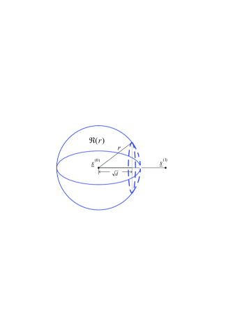
Figure 1: The geometric interpretation of the SB.

III-A1 Nested Regions

The SB chooses the nested regions to be a family of $n$-dimensional spheres centered at the transmitted signal vector, that is, $\mathcal{R}(r)=\{\underline{y}\mid\|\underline{y}-\underline{s}^{(0)}\|\leq r\}$, where $r\geq 0$ is the parameter.

III-A2 Probability Density Function of the Parameter

The pdf of the parameter is

$$g(r)=\frac{2r^{n-1}e^{-\frac{r^{2}}{2\sigma^{2}}}}{2^{\frac{n}{2}}\sigma^{n}\Gamma(\frac{n}{2})},~{}~{}r\geq 0.$$ (12)

III-A3 Conditional Upper Bound

The SB chooses $f_{u}(r)$ to be the conditional union bound. Given that $||{\underline{y}}-{\underline{s}}^{(0)}||=r$, $\underline{y}$ is uniformly distributed over $\partial\mathcal{R}(r)$. Hence the conditional pair-wise error probability $p_{2}(r,d)$ does not depend on the SNR and can be evaluated as the ratio of the surface area of a spherical cap to that of the whole sphere, as shown in Fig. 1. That is,

$$\!\!\!\!\!p_{2}(r,d)\!\!=\!\!\left\{\begin{array}[]{rl}\frac{\Gamma(\frac{n}{2})}{\sqrt{\pi}~{}\Gamma(\frac{n-1}{2})}\int_{0}^{\arccos(\frac{\sqrt{d}}{r})}\sin^{n-2}\phi~{}{\rm d}\phi,&r>\sqrt{d}\\ 0,&r\leq\sqrt{d}\end{array}\right.,$$ (13)

which is a non-decreasing and continuous function of $r$ such that $p_{2}(0,d)=0$ and $p_{2}(+\infty,d)=1/2$. Therefore, the conditional union bound

$$f_{u}(r)=\sum_{1\leq d\leq n}A_{d}p_{2}(r,d)$$ (14)

is also an non-decreasing and continuous function of $r$ such that $f_{u}(0)=0$ and $f_{u}(+\infty)\geq 3/2$. Furthermore, $f_{u}(r)$ is a strictly increasing function in the interval $[\sqrt{d_{\min}},+\infty)$ with $f_{u}(\sqrt{d_{\min}})=0$. Hence there exists a unique $r_{1}$ satisfying

$$\sum_{1\leq d\leq n}A_{d}p_{2}(r,d)=1,$$ (15)

which is equivalent to that given in [13, (3.48)] by noticing that $p_{2}(r,d)=0$ for $d>r^{2}$.

III-A4 Equivalence

The SB can be written as

$${\rm Pr}\{E\} \leq \int_{0}^{r_{1}}f_{u}(r)g(r)~{}{\rm d}r+\int_{r_{1}}^{+\infty}g(r)~{}{\rm d}r$$ (16)

$$= \int_{0}^{+\infty}\min\{f_{u}(r),1\}g(r)~{}{\rm d}r,$$

where $g(r)$ and $f_{u}(r)$ are given in (12) and (14), respectively. The optimal parameter $r_{1}$ is given by solving the equation (15), which does not depend on the SNR. It can be seen that (16) is exactly the sphere bound of Kasami et al [2][3]. It can also be proved that (16) is equivalent to that given in [13, (3.45)-(3.48)]. Firstly, we have shown that the optimal radius $r_{1}$ satisfies (15), which is equivalent to that given in [13, (3.48)]. Secondly, by changing variables, $z_{1}=r\cos\phi$ and $y=r^{2}$, it can be verified that (16) is equivalent to that given in [13, Sec.3.2.5].

III-B The Tangential Bound Revisited

The AWGN sample $\underline{z}$ can be separated by projection as a radial component $z_{\xi_{1}}$ and $n-1$ tangential (orthogonal) components $\{z_{\xi_{i}},2\leq i\leq n\}$. Specifically, we set $z_{\xi_{1}}$ to be the inner product of $\underline{z}$ and $-{\underline{s}}^{(0)}/\sqrt{n}$. When considering the pair-wise error probability, we assume that $z_{\xi_{2}}$ is the component that lies in the plane determined by ${\underline{s}}^{(0)}$ and ${\underline{s}}^{(1)}$.

III-B1 Nested Regions

The TB chooses the nested regions to be a family of half-spaces $Z_{\xi_{1}}\leq z_{\xi_{1}}$, where $z_{\xi_{1}}\in\mathbb{R}$ is the parameter.

III-B2 Probability Density Function of the Parameter

The pdf of the parameter is

$$g(z_{\xi_{1}})=\frac{1}{\sqrt{2\pi}\sigma}e^{-\frac{z_{\xi_{1}}^{2}}{2\sigma^{2}}}.$$ (17)

III-B3 Conditional Upper Bound

The TB chooses $f_{u}(z_{\xi_{1}})$ to be the conditional union bound. Given that $Z_{\xi_{1}}=z_{\xi_{1}}$, the conditional pair-wise error probability is given by

$$p_{2}(z_{\xi_{1}},d)=\int_{\frac{\sqrt{d}(\sqrt{n}-z_{\xi_{1}})}{\sqrt{n-d}}}^{+\infty}\frac{1}{\sqrt{2\pi}\sigma}e^{-\frac{z_{\xi_{2}}^{2}}{2\sigma^{2}}}~{}{\rm d}z_{\xi_{2}},$$ (18)

which is a strictly increasing and continuous function of $z_{\xi_{1}}$ such that $p_{2}(-\infty,d)=0$ and $p_{2}(\sqrt{n},d)=1/2$. Then the conditional union bound is given by

$$f_{u}(z_{\xi_{1}})=\sum_{d=1}^{n}A_{d}p_{2}(z_{\xi_{1}},d),$$ (19)

which is also strictly increasing and continuous function of $z_{\xi_{1}}$ such that $f_{u}(-\infty)=0$ and $f_{u}(\sqrt{n})\geq 3/2$. Hence there exists a unique solution $z_{\xi_{1}}^{*}\leq\sqrt{n}$ satisfying

$$\sum_{d=1}^{n}A_{d}p_{2}(z_{\xi_{1}},d)=1,$$ (20)

which is equivalent to that given in [13, (3.22)] by noticing that $p_{2}(z_{\xi_{1}},d)=Q\left(\frac{\sqrt{d}(\sqrt{n}-z_{\xi_{1}})}{\sigma\sqrt{n-d}}\right)$ and $d=\delta_{d}^{2}/4$.

III-B4 Equivalence

The TB can be written as

$${\rm Pr}\{E\} \leq \int_{-\infty}^{z_{\xi_{1}}^{*}}\!\!\!f_{u}(z_{\xi_{1}})g(z_{\xi_{1}})~{}{\rm d}z_{\xi_{1}}+\int_{z_{\xi_{1}}^{*}}^{+\infty}\!\!\!\!\!g(z_{\xi_{1}})~{}{\rm d}z_{\xi_{1}}$$ (21)

$$= \int_{-\infty}^{+\infty}\min\{f_{u}(z_{\xi_{1}}),1\}g(z_{\xi_{1}})~{}{\rm d}z_{\xi_{1}},$$

where $g_{(}z_{\xi_{1}})$ and $f_{u}(z_{\xi_{1}})$ are given in (17) and (19), respectively. The optimal parameter $z_{\xi_{1}}^{*}$ is given by solving the equation (20). It can be shown that (21) is equivalent to that given in [13, (3.21)].

III-C The Tangential-Sphere Bound Revisited

Assume that $n\geq 3$.

III-C1 Nested Regions

Again, the TSB chooses the nested regions to be a family of half-spaces $Z_{\xi_{1}}\leq z_{\xi_{1}}$, where $z_{\xi_{1}}\in\mathbb{R}$ is the parameter.

III-C2 Probability Density Function of the Parameter

The pdf of the parameter is

$$g(z_{\xi_{1}})=\frac{1}{\sqrt{2\pi}\sigma}e^{-\frac{z_{\xi_{1}}^{2}}{2\sigma^{2}}}.$$ (22)

III-C3 Conditional Upper Bound

Different from the TB, the TSB chooses $f_{u}(z_{\xi_{1}})$ to be the conditional sphere bound. The conditional sphere bound given that $Z_{\xi_{1}}=z_{\xi_{1}}$ can be derived as follows.

Let $\mathcal{R}(r)$ be the $(n-1)$-dimensional sphere of radius $r>0$ which is centered at $(1-z_{\xi_{1}}/\sqrt{n})s^{(0)}$ and located inside the hyper-plane $Z_{\xi_{1}}=z_{\xi_{1}}$.

• Case 1: $Z_{\xi_{1}}=z_{\xi_{1}}\geq\sqrt{n}$. It can be shown that, given that received vector falls on $\partial\mathcal{R}(r)$, the pair-wise error probability is no less than 1/2. Hence the conditional union bound is no less than 3/2. From Theorem 1, we know that the optimal radius $r_{1}(z_{\xi_{1}})=0$, which results in the trivial upper bound $f_{u}(z_{\xi_{1}})\equiv 1$.

• Case 2: Given that $Z_{\xi_{1}}=z_{\xi_{1}}<\sqrt{n}$, the ML decoding error probability can be evaluated by considering an equivalent system in which each bipolar codeword is scaled by a factor $(\sqrt{n}-z_{\xi_{1}})/\sqrt{n}$ before transmitted over an AWGN channel with (projective) noise $(0,Z_{\xi_{2}},\cdots,Z_{\xi_{n}})$. The system is also equivalent to transmission of the original codewords over an AWGN but with scaled (projective) noise $\sqrt{n}/(\sqrt{n}-z_{\xi_{1}})(0,Z_{\xi_{2}},\cdots,Z_{\xi_{n}})$. The latter reformulation allows us to get the conditional sphere bound easily since the optimal radius is independent of the SNR. Actually, we notice that, given that the noise falls on the $(n-1)$-dimensional sphere $\partial\mathcal{R}(r)$ in the hyper-plane $z_{\xi_{1}}=0$, the conditional pair-wise error probability is

  $$\!\!\!\!\!p_{2}(r,d)\!\!=\!\!\frac{\Gamma(\frac{n-1}{2})}{\sqrt{\pi}~{}\Gamma(\frac{n-2}{2})}\int_{0}^{\arccos(\frac{\sqrt{nd/(n-d)}}{r})}\sin^{n-3}\phi~{}{\rm d}\phi$$

  if $r>\sqrt{nd/(n-d)}$ and $p_{2}(r,d)=0$ otherwise. Then we have the conditional sphere bound

  $$f_{u}(z_{\xi_{1}})=\int_{0}^{r_{1}}f_{s}(r)g_{s}(z_{\xi_{1}},r)~{}{\rm d}r+\int_{r_{1}}^{+\infty}g_{s}(z_{\xi_{1}},r)~{}{\rm d}r,$$ (23)

  where

  $$g_{s}(z_{\xi_{1}},r)=\frac{2r^{n-2}e^{-\frac{r^{2}}{2\tilde{\sigma}^{2}}}}{2^{\frac{n-1}{2}}\tilde{\sigma}^{n-1}\Gamma(\frac{n-1}{2})},~{}~{}r\geq 0,$$ (24)

  which depends on the SNR via $\tilde{\sigma}=\sqrt{n}\sigma/(\sqrt{n}-z_{\xi_{1}})$, and

  $$\!\!\!\!f_{s}(r)=\!\!\!\!\!\sum_{1\leq d\leq\frac{r^{2}n}{r^{2}+n}}A_{d}\frac{\Gamma(\frac{n-1}{2})}{\sqrt{\pi}~{}\Gamma(\frac{n-2}{2})}\int_{0}^{\arccos(\frac{\sqrt{nd/(n-d)}}{r})}\!\!\!\!\!\!\sin^{n-3}\phi~{}{\rm d}\phi,$$ (25)

  which is independent of $\tilde{\sigma}$, as justified previously. The optimal radius $r_{1}$ is the unique solution of

  $$\sum_{1\leq d\leq\frac{r^{2}n}{r^{2}+n}}A_{d}\frac{\Gamma(\frac{n-1}{2})}{\sqrt{\pi}~{}\Gamma(\frac{n-2}{2})}\int_{0}^{\arccos(\frac{\sqrt{nd/(n-d)}}{r})}\!\!\!\!\!\!\sin^{n-3}\phi~{}{\rm d}\phi=1.$$ (26)

  Since $r_{1}<+\infty$, $f_{u}(z_{\xi_{1}})<1$ for all $z_{\xi_{1}}<\sqrt{n}$.

• Summary: We have shown that the conditional sphere upper bound such that $f_{u}(z_{\xi_{1}})<1$ if $z_{\xi_{1}}<\sqrt{n}$; otherwise, $f_{u}(z_{\xi_{1}})=1$. Hence the optimal parameter $z_{\xi_{1}}^{*}=\sqrt{n}$.

III-C4 Equivalence

The TSB can be written as

$${\rm Pr}\{E\}\!\!\! \leq \!\!\!\int_{-\infty}^{\sqrt{n}}\!\!\!\!\!f_{u}(z_{\xi_{1}})g(z_{\xi_{1}})~{}{\rm d}z_{\xi_{1}}+\int_{\sqrt{n}}^{+\infty}\!\!\!\!\!g(z_{\xi_{1}})~{}{\rm d}z_{\xi_{1}},$$ (27)

where $g(z_{\xi_{1}})$ is given by (22), and $f_{u}(z_{\xi_{1}})$ is given by (23)-(26).

To prove the equivalence of (27) to the formulae given in  [13, Sec.3.2.1], we first show that the optimal region is the same as that given in [13, Sec.3.2.1]. Noting that the optimal radius $r_{1}$ satisfies (26), which is equivalent to that given in [13, (3.12)]. Back to the hyper-plane $Z_{\xi_{1}}=z_{\xi_{1}}$, we can see that the optimal parameter is $r_{1}(\sqrt{n}-z_{\xi_{1}})/\sqrt{n}$. This means that the optimal region is a half-cone with the same angle as that given in [13, (3.12)]. Then, by changing variables, $r^{\prime}=r(\sqrt{n}-z_{\xi_{1}})/\sqrt{n}$, $z_{\xi_{2}}=r^{\prime}\cos\phi$, $v=r^{\prime 2}-z_{\xi_{2}}^{2}$ and $y=r^{\prime 2}$, it can be verified that (27) is equivalent to that given in [13, (3.10)], except that the second term ${\rm Pr}\{Z_{\xi_{1}}\geq\sqrt{n}\}$. This term did not appear in the original derivation of TSB in [5], but is required as pointed out in [16, Appendex A].

IV Conclusions

In this paper, we have presented a general framework to investigate Gallager’s first bounding technique with a single parameter. We have presented a sufficient and necessary condition for the optimal parameter. With the proposed general framework, we have re-derived three well-known bounds and presented the relationships among them. We have also revealed a fact that the SB of Herzberg and Poltyrev is equivalent to the SB of Kasami et al.

References

• [1] E. R. Berlekamp, “The technology of error correction codes,” Proceedings of the IEEE, vol. 68, pp. 564–593, May 1980.
• [2] T. Kasami, T. Fujiwara, T. Takata, K. Tomita, and S. Lin, “Evaluation of the block error probability of block modulation codes by the maximum-likelihood decoding for an AWGN channel,” in Proc. of the 15th Symposium on Information Theory and Its Applications, Minakami, Japan, September 1992.
• [3] T. Kasami, T. Fujiwara, T. Takata, and S. Lin, “Evaluation of the block error probability of block modulation codes by the maximum-likelihood decoding for an AWGN channel,” in Proc. 1993 IEEE Int. Symp. Inform. Theory, January 1993, p. 68.
• [4] H. Herzberg and G. Poltyrev, “Techniques of bounding the probability of decoding error for block coded modulation structures,” IEEE Transactions on Information Theory, vol. 40, pp. 903–911, May 1994.
• [5] G. Poltyrev, “Bounds on the decoding error probability of binary linear codes via their spectra,” IEEE Transactions on Information Theory, vol. 40, pp. 1284–1292, July 1994.
• [6] D. Divsalar, “A simple tight bound on error probability of block codes with application to turbo codes,” in Proc. 1999 IEEE Communication Theory Workshop, Aptos, CA, May 1999.
• [7] D. Divsalar and E. Biglieri, “Upper bounds to error probabilities of coded systems beyond the cutoff rate,” IEEE Trans. Commun., vol. 51, no. 12, pp. 2011–2018, December 2003.
• [8] S. Yousefi and A. K. Khandani, “A new upper bound on the ML decoding error probability of linear binary block codes in AWGN interference,” IEEE Transactions on Information Theory, vol. 50, pp. 3026–3036, Novomber 2004.
• [9] ——, “Generalized tangential sphere bound on the ML decoding error probability of linear binary block codes in AWGN interference,” IEEE Transactions on Information Theory, vol. 50, pp. 2810–2815, Novomber 2004.
• [10] A. Mehrabian and S. Yousefi, “Improved tangential sphere bound on the ML decoding error probability of linear binary block codes in AWGN and block fading channels,” IEE Proc. Commun., vol. 153, pp. 885–893, December 2006.
• [11] X. Ma, C. Li, and B. Bai, “Maximum likelihood decoding analysis of LT codes over AWGN channels,” in Proc. of the 6th International Symposium on Turbo Codes and Iterative Information Processing, Brest, France, September 2010.
• [12] X. Ma, J. Liu, and B. Bai, “New techniques for upper-bounding the MLD performance of binary linear codes,” in Proc. 2011 IEEE Int. Symp. Inform. Theory, Saint-Petersburg, Russian Federation, August 2011.
• [13] I. Sason and S. Shamai, “Performance analysis of linear codes under maximum-likelihood decoding: A tutorial,” in Foundations and Trends in Communications and Information Theory.   Delft, The Netherlands: NOW, July 2006, vol. 3, no. 1-2, pp. 1–225.
• [14] E. Agrell, “Voronoi regions for binary linear block codes,” IEEE Transactions on Information Theory, vol. 42, pp. 310–316, January 1996.
• [15] ——, “On the Voronoi neighbor ratio for binary linear block codes,” IEEE Transactions on Information Theory, vol. 44, pp. 3064–3072, Novomber 1998.
• [16] I. Sason and S. Shamai, “Improved upper bounds on the ML decoding error probability of parallel and serial concatenated turbo codes via their ensemble distance spectrum,” IEEE Transactions on Information Theory, vol. 46, pp. 24–47, January 2000.