Fractional Calculus
in Wave Propagation Problems

This paper, presented as an invited lecture at Fest-Kolloquium for celebrating the 80-th anniversary of Prof. Dr. Rudolf Gorenflo, held at the Free University of Berlin on 24 June 2011, has been published in Forum der Berliner Mathematischer Gesellschaft, Vol 19, pp. 20–52 (2011).

Dedicated to Professor Rudolf Gorenflo

on the occasion of his 80th anniversary

Abstract

Fractional calculus, in allowing integrals and derivatives of any positive order (the term "fractional" kept only for historical reasons), can be considered a branch of mathematical physics which mainly deals with integro-differential equations, where integrals are of convolution form with weakly singular kernels of power law type. In recent decades fractional calculus has won more and more interest in applications in several fields of applied sciences. In this lecture we devote our attention to wave propagation problems in linear viscoelastic media. Our purpose is to outline the role of fractional calculus in providing simplest evolution processes which are intermediate between diffusion and wave propagation. The present treatment mainly reflects the research activity and style of the author in the related scientific areas during the last decades.

Sommario

Il calcolo frazionario tratta di integrali e derivate di ordine positivo qualsiasi. Si noti che il termine "frazionario" è mantenuto solo per ragioni storiche. Esso può essere considerato una branca della Fisica Matematica che principalmente analizza equazioni integro-differenziali in cui gli integrali sono di tipo convolutivo con nuclei debolmente singolari a legge di potenza. Recentemente il calcolo frazionario ha acquistato un interesse crescente per le applicazioni che trova in vari campi delle scienze applicate. In questa lezione noi rivolgiamo l’attenzione a problemi di propagazione ondosa in mezzi lineari viscoelastici. Il nostro proposito è di sottolineare il ruolo del calcolo frazionario nel fornire semplici processi di evoluzione che sono intermedi tra la diffusione e la propagazione di onde. Il trattamento presente si basa principalmente sull’attività di ricerca dell’autore.

1 Introduction

In this lecture we devote our attention to the applications of fractional calculus in providing the simplest evolution processes which are intermediate between diffusion and wave propagation. As an example we consider special linear viscoelastic media that, by exhibiting power law creep, turn out to be intermediate models between viscous fluids (diffusion) and elastic solids (waves).

We start to consider the family of evolution equations obtained from the standard diffusion equation (or the D’Alembert wave equation) by replacing the first-order (or the second-order) time derivative by a fractional derivative (in the Caputo sense) of order $\beta$ with $0<\beta\leq 2\,,$ namely

   $${{\partial^{\beta}w\over\partial t^{\beta}}=a\,{\partial^{2}w\over\partial x^{2}}\,,\qquad a>0\,,\quad 0<\beta\leq 2\,,}$$   

where $x\in S\subset\vbox{\hbox to8.9pt{I\hskip-2.1ptR\hfil}}$, $t\in\vbox{\hbox to8.9pt{I\hskip-2.1ptR\hfil}}^{+}$ denote the space and time variables, respectively.

In Eq. (1.1) $w(x,t)$ represents the response field variable, $a$ is a positive constant of dimension $L^{2}\,T^{-\beta}\,.$ For essentials on the Caputo fractional derivative we refer the reader to the appendix; more details can be found in the literature on fractional calculus, see e.g. Gorenflo & Mainardi (1997), Podlubny (1999), Kilbas, Srivastave & Trujillo (2006).

It is necessary to keep distinct the cases

$$0<\beta\leq 1\,,\quad\hbox{and}\quad 1<\beta\leq 2\,,$$

by recalling

for $0<\beta<1$ :

   $${{\partial^{\beta}w\over\partial t^{\beta}}:=\ {\displaystyle{1\over{\Gamma(1-\beta)}}}\,{\displaystyle\int_{0}^{t}}\left[{\displaystyle{\partial\over\partial\tau}}\,w(x,\tau)\right]\,{\displaystyle{d\tau\over(t-\tau)^{\beta}}}\,,}$$   

for $1<\beta<2$ :

   $${{\partial^{\beta}w\over\partial t^{\beta}}:={\displaystyle{1\over{\Gamma(2-\beta)}}}\,{\displaystyle\int_{0}^{t}}\left[{\displaystyle{\partial^{2}\over\partial\tau^{2}}}\,w(x,\tau)\right]\,{\displaystyle{d\tau\over(t-\tau)^{\beta-1}}}\,,}$$   

where $\Gamma$ denotes the Gamma function.

We also outline that the expression in the R.H.S. of (1.2) as $\beta\to 1^{-}$ reduces to the standard derivative of order 1, whereas the corresponding expression in (1.3) as $\beta\to 2^{-}$ reduces to the standard derivatives of order 2.

It should be noted that for $0<\beta<1$ and $1<\beta<2$, in view of (1.2) and (1.3), Eq (1.1) turns out to be an integro-differential equation with a weakly singular kernel. The singularities can be removed by a suitable fractional integration in time, taking into account the necessary initial conditions at $t=0^{+}$. Consequently we get the integro-differential equations

for $0<\beta\leq 1$ :

$$w(x,t)=w(x,0^{+})+{\displaystyle{a\over\Gamma(\beta)}}\,{\displaystyle\int_{0}^{t}}\left({\displaystyle{\partial^{2}w\over\partial x^{2}}}\right)\,(t-\tau)^{\beta-1}\,d\tau\,;$$

for $1<\beta\leq 2$ :

$$\begin{array}[]{ll}w(x,t)=&w(x,0^{+})+t\,w_{t}(x,0^{+})\\ &+{\displaystyle{a\over\Gamma(\beta)}}\,{\displaystyle\int_{0}^{t}}\left({\displaystyle{\partial^{2}w\over\partial x^{2}}}\right)(t-\tau)^{\beta-1}\,\,d\tau\,.\end{array}$$

There is huge literature concerning evolution equations of the types discussed above, both with and without reference to the fractional calculus. We quote a number of references in the last decades of the past century, that have mostly attracted our attention, e.g., Caputo (1969, 1996), Meshkov & Rossikhin (1970), Pipkin (1972-1986), Gonovskii & Rossikhin (1973), Buchen & Mainardi (1975), Kreis & Pipkin (1986), Nigmatullin (1986), Fujita (1989a,1989b), Schneider & Wyss (1989), Kochubei (1990), Giona & Roman (1992), Prüsse (1993), Metzler et al. (1994), Engler (1997), Rossikhin & Shitikova (1997, 2007, 2010). This talk is a brief survey of my work carried out since 1993 when I started to re-consider wave propagation problems by using the methods of the fractional calculus

The plan of the lecture is as follows.

In Section 2 we derive the general evolution equation governing the propagation of uniaxial stress waves, in the framework of the dynamical theory of linear viscoelasticity. For a power-law solid exhibiting a creep law proportional to $t^{\gamma}$ ($0<\gamma<1$) the evolution equation is shown to be of type (1.1) with

$$1<\beta:=2-\gamma<2\,.$$

In Section 3 we review the analysis of the fractional evolution equation (1.1) in the general case $0<\beta<2\,.$

We first analyze the two basic boundary-value problems referred to as the Cauchy problem and the Signalling problem, by the technique of the Laplace transforms and we derive the transformed expressions of the respective fundamental solutions (the Green functions).

Then, we carry out the inversion of the relevant transforms and we outline a reciprocity relation between the Green functions in the space-time domain.

In view of this relation the Green functions can be expressed in terms of two interrelated auxiliary functions in the similarity variable $r=|x|/(\sqrt{a}t^{\nu})\,,$ where $\nu=\beta/2\,.$ These auxiliary functions can be analytically continued in the whole complex plane as entire functions of Wright type.

In Section 4 we outline the scaling properties of the fundamental solutions and we exhibit their evolution for some values of the order $\beta\,.$ For $1<\beta<2$ the behaviour of the fundamental solutions turns out to be intermediate between diffusion (found for a viscous fluid) and wave-propagation (found for an elastic solid), thus justifying the attribute of fractional diffusive waves.

In Section 5 the fundamental solutions are interpreted as probability density functions related to Lévy stable processes with index of stability depending on $\beta\,.$

In Appendix A we recall the essentials of the time–fractional differentiation whereas in Appendix B we exhibit some graphical representations of the relevant Wright function.

2 Linear viscoelastic waves and
the fractional diffusion-wave equation

According to the elementary one-dimensional theory of linear viscoelasticity, the medium is assumed to be homogeneous (of density $\rho$), semi-infinite or infinite in extent ($0\leq x<+\infty$ or $-\infty<x<+\infty$) and undisturbed for $t<0\,.$

The basic equations are known to be, see e.g. Hunter (1960), Caputo & Mainardi (1971b), Pipkin (1972-1986), Christensen (1972-1982), Chin (1980), Graffi (1982),

$$\sigma_{x}(x,t)=\rho\,u_{tt}(x,t)\,,$$

$$\varepsilon(x,t)=u_{x}(x,t)\,,$$

$$\varepsilon(x,t)=[J_{0}+\dot{J}(t)*\,]\,\sigma(x,t)\,.$$

The following notations have been used: $\sigma$ for the stress, $\varepsilon$ for the strain, $J(t)$ for the creep compliance (the strain response to a unit step input of stress); the constant $J_{0}:=J(0^{+})\geq 0$ denotes the instantaneous (or glass) compliance.

The evolution equation for the response variable $w(x,t)$ (chosen among the field variables: the displacement $u$, the stress $\sigma$, the strain $\varepsilon$ or the particle velocity $v=u_{t}$) can be derived through the application of the Laplace transform to the basic equations.

$${\cal{L}}\,\left\{f(t);s\right\}:=\int_{0}^{\infty}\!\!{\rm e}^{-st}\,f(t)\,dt=\widetilde{f}(s)\div f(t)\,,\quad s\in{\rm C\hskip-4.8pt\vrule height=6.0pt,width=0.1831pt\hskip 5.0pt}\,.$$

We first obtain in the transform domain, the second order differential equation

   $${\left[{d^{2}\over dx^{2}}-\mu^{2}(s)\right]\,\widetilde{w}(x,s)=0\,,}$$   

in which

$$\mu(s):=s\,\left[\rho\,s{\widetilde{J}(s)}\right]^{1/2}\,,$$

is real and positive for $s$ real and positive. As a matter of fact, $\mu(s)$ turns out to be an analytic function of $s$ over the entire $s$-plane cut along the negative real axis; the cut can be limited or unlimited in accordance with the particular viscoelastic model assumed.

Wave-like or diffusion-like character of the evolution equation can be drawn from (2.5) by taking into account the asymptotic representation of the creep compliance for short times,

   $${J(t)=J_{0}+O(t^{\gamma})\,,\quad{\rm as}\;t\to 0^{+}\,,}$$   

with $J_{0}\geq 0\,,$ and $0<\gamma\leq 1\,.$

If $J_{0}>0$ then

$$\lim_{s\to\infty}{\mu(s)\over s}=\sqrt{\rho J_{0}}:={1\over c}\,,$$

we have a wave like behaviour with $c$ as the wave-front velocity; otherwise ($J_{0}=0)$ we have a diffusion like behaviour.

In the case $J_{0}>0$ the wave-like evolution equation for $w(x,t)$ can be derived by inverting (2.4-5), using (2.6-7) and introducing the non-dimensional rate of creep

$$\psi(t):={1\over J_{0}}\,{dJ(t)\over dt}\geq 0\,,\quad t>0\,.$$

We get

$$\mu^{2}(s):=s^{2}[\rho\,s{\widetilde{J}(s)}]=[1+\widetilde{\psi}(s)]\,{s^{2}\over c^{2}}\,,$$

so that the evolution equation turns out as

   $${\left\{1+\psi(t)\,*\,\right\}\,{\partial^{2}w\over\partial t^{2}}=c^{2}\,{\partial^{2}w\over\partial x^{2}}\,.}$$   

This is a generalization of D’Alembert wave equation in that it is an integro-differential equation where the convolution integral can be interpreted as a perturbation term. This case has been investigated by Buchen and Mainardi (1975) and by Mainardi and Turchetti (1975), who have provided wave-front expansions for the solutions.

In the case $J_{0}=0$ we can re-write (2.6) as

   $${J(t)={1\over\rho\,a}\,{t^{\gamma}\over\Gamma(\gamma+1)}+o\,(t^{\gamma})\,,\quad{\rm as}\;t\to 0^{+}\,,}$$   

where, for convenience, we have introduced the positive constant $a$ (with dimension $L^{2}\,T^{\gamma-2}$) and the Gamma function $\Gamma(\gamma+1)\,.$ Then we can introduce the non-dimensional function $\phi(t)$ whose Laplace transform is such that

$$\mu^{2}(s):=s^{2}\,[\rho\,s{\widetilde{J}(s)}]=[1+\widetilde{\phi}(s)]\,{s^{2-\gamma}\over a}\,.$$

Using (2.12), the Laplace inversion of (2.4-5) yields

   $${\left[1+\phi(t)\,*\,\right]\,{\partial^{\beta}w\over\partial t^{\beta}}=a\,{\partial^{2}w\over\partial x^{2}}\,,\quad\beta=2-\gamma\,,}$$   

so that, being $0<\gamma\leq 1$, we have $1\leq\beta<2$.

When the creep compliance satisfies the simple power-law

   $${J(t)={1\over\rho\,a}\,{t^{\gamma}\over\Gamma(\gamma+1)}\,,\quad 0<\gamma\leq 1\,,\quad t>0\,,}$$   

we obtain $\mu^{2}(s)=s^{2-\gamma}/a$ so $\phi(t)\equiv 0\,.$ As a consequence the evolution equation (2.13) simply reduces to Eq. (1.1). As pointed out by Caputo and Mainardi (1971b), the creep law (2.14) is provided by viscoelastic models whose stress-strain relation (2.3) can be simply expressed by a fractional derivative of order $\gamma\,.$ In the present notation this stress-strain relation reads

   $${\sigma={\rho\,a}\,{d^{\gamma}\over dt^{\gamma}}\,\varepsilon\,,\quad 0<\gamma\leq 1\,.}$$   

For $\gamma=1$ the Newton law for a viscous fluid is recovered from (2.15) where $a$ now represents the kinematic viscosity; in this case, since $\beta=1$ in (1.2), the classical diffusion equation holds for $w(x,t)\,.$

In the limiting case $\gamma=0$ we obtain from (2.14)

$$J(t)=J_{0}=1/(\rho\,a)$$

so we recover from (2.10) and (2.12) the classical D’Alembert wave equation ($\beta=2$) with wave front velocity $c=\sqrt{a}\,.$

When $0<\gamma<1$ we just obtain the evolution equation (1.1) with $1<\beta<2$ In this case, as we have previously pointed out, being intermediate between the heat equation and the wave equation, Eq. (1.1) is referred to as the fractional diffusion-wave equation, and its solutions can be interpreted as fractional diffusive waves, see Mainardi (1995), Mainardi & Paradisi (2001).

We point out that the viscoelastic models based on (2.14) or (2.15) with $0<\gamma<1$ and henceforth governed by the fractional diffusion-wave equation, are of great interest in material sciences and seismology. In fact, as shown by Caputo & Mainardi (1971b) and then by Caputo (1973, 1976, 1979), these models exhibit an internal friction independent on frequency according to the law

   $${Q^{-1}={\rm tan}\,\left(\gamma\,\pi\over 2\right)\,\Longleftrightarrow\,\gamma={2\over\pi}\,{\rm arctan}\,\left(Q^{-1}\right)\,.}$$   

The independence of the $Q$ from the frequency is in fact experimentally verified in pulse propagation phenomena for many materials, see Kolsky (1956) including those of seismological interest, see Kjiartansoon (1979), Strick (1970, 1982), Strick and Mainardi (1982).

From (2.16) we note that $Q$ is also independent on the material constants $\rho$ and $a$ which, however, play a role in the phenomenon of wave dispersion.

The limiting cases of absence of energy dissipation (the elastic energy is fully stored) and of absence of energy storage (the elastic energy is fully dissipated) are recovered from (2.16) for $\gamma=0\,$ (perfectly elastic solid) and $\gamma=1\,$ (perfectly viscous fluid), respectively.

To obtain values of seismological interest for the dissipation ($Q\approx 1000$) we need to choose the parameter $\gamma$ sufficiently close to zero, which corresponds to a nearly elastic material; from (2.16) we obtain the approximate relations between $\gamma$ and $Q\,,$ namely

   $${\gamma\approx\left({2\over\pi\,Q}\right)\approx 0.64Q^{-1}\Longleftrightarrow Q^{-1}\approx{\pi\over 2}\gamma\approx 1.57\gamma.}$$   

3 Derivation of the fundamental solutions

In order to guarantee the existence and the uniqueness of the solution, we must equip (1.1) with suitable data on the boundary of the space-time domain.

The basic boundary-value problems for diffusion are the so-called Cauchy and Signalling problems.

In the Cauchy problem, which concerns the space-time domain $-\infty<x<+\infty\,,$ $\,t\geq 0\,,$ the data are assigned at $t=0^{+}$ on the whole space axis (initial data).

In the Signalling problem, which concerns the space-time domain $x\geq 0\,,$ $\,t\geq 0\,,$ the data are assigned both at $t=0^{+}$ on the semi-infinite space axis $x>0$ (initial data) and at $x=0^{+}$ on the semi-infinite time axis $t>0$ (boundary data); here, as mostly usual, the initial data are assumed to vanish.

Denoting by $f(x)\,,\,x\in\vbox{\hbox to8.9pt{I\hskip-2.1ptR\hfil}}\,$ and $\,h(t)\,,\,t\in\vbox{\hbox to8.9pt{I\hskip-2.1ptR\hfil}}^{+}\,$ sufficiently well-behaved functions, the basic problems are thus formulated as following, assuming $0<\beta\leq 1\,$:

a) Cauchy problem

$$\begin{cases}w(x,0^{+})=f(x)\,,\quad-\infty<x<+\infty\,;\\ w(\mp\infty,t)=0\,,\quad\,t>0\,;\end{cases}$$

b) Signalling problem

$$\begin{cases}w(x,0^{+})=0\,,\quad x>0\,;\\ w(0^{+},t)=h(t)\,,\;w(+\infty,t)=0\,,\quad t>0\,.\end{cases}$$

If $1<\beta<2\,,$ we must add in (3.1a) and (3.1b) the initial values of the first time derivative of the field variable, $w_{t}(x,0^{+})\,,$ since in this case the fractional derivative is expressed in terms of the second order time derivative. To ensure the continuous dependence of our solution with respect to the parameter $\beta$ also in the transition from $\beta=1^{-}$ to $\beta=1^{+}\,,$ we agree to assume

$$w_{t}(x,0^{+})=0\,,\quad\hbox{for}\quad 1<\beta\leq 2\,,$$

as it turns out from the integral forms (1.4)-(1.5).

In view of our subsequent analysis we find it convenient to set

$$\nu:={\beta/2}\,,\quad{\hbox{so}}\quad\begin{cases}0<\nu\leq 1/2\,,\;if\;0<\beta\leq 1\,,\\ 1/2<\nu\leq 1\,,\;if\;1<\beta\leq 2\,,\end{cases}$$

and from now on to add the parameter $\nu$ to the independent space-time variables $x\,,\,t$ in the solutions, writing $w=w(x,t;\nu)\,.$

For the Cauchy and Signalling problems we introduce the so-called Green functions ${\cal{G}}_{c}(x,t;\nu)$ and ${\cal{G}}_{s}(x,t;\nu)$, which represent the respective fundamental solutions, obtained when $f(x)=\delta(x)$ and $h(t)=\delta(t)\,.$ As a consequence, the solutions of the two basic problems are obtained by a space or time convolution according to

$$w(x,t;\nu)=\int_{-\infty}^{+\infty}{\cal{G}}_{c}(x-\xi,t;\nu)\,f(\xi)\,d\xi\,,$$

$$w(x,t;\nu)=\int_{0^{-}}^{t^{+}}{\cal{G}}_{s}(x,t-\tau;\nu)\,h(\tau)\,d\tau\,.$$

It should be noted that in (3.3a) ${\cal{G}}_{c}(x,t;\nu)={\cal{G}}_{c}(|x|,t;\nu)$ since the Green function of the Cauchy problem turns out to be an even function of $x$. According to a usual convention, in (3.3b) the limits of integration are extended to take into account for the possibility of impulse functions centred at the extremes. For the standard diffusion equation ($\nu=1/2$) it is well known that

$${\cal{G}}_{c}(x,t;1/2):={\cal{G}}_{c}^{d}(x,t)={t^{-1/2}\over 2\sqrt{\pi a}}\,{\rm e}^{-\displaystyle x^{2}/(4\,a\,t)}\,,$$

$${\cal{G}}_{s}(x,t;1/2):={\cal{G}}_{s}^{d}(x,t)={x\,t^{-3/2}\over 2\sqrt{\pi a}}\,{\rm e}^{-\displaystyle x^{2}/(4\,a\,t)}\,.$$

In the limiting case $\nu=1$ we recover the standard wave equation, for which, putting $c=\sqrt{a}\,,$

$${\cal{G}}_{c}(x,t;1):={\cal{G}}_{c}^{w}(x,t)={1\over 2}\left[\delta(x-ct)+\delta(x+ct)\right]\,,$$

$${\cal{G}}_{s}(x,t;1):={\cal{G}}_{s}^{w}(x,t)=\delta(t-x/c)\,.$$

In the general case $0<\nu<1$ the two Green functions will be determined by using the technique of the Laplace transform.

For the Cauchy problem (3.1a) with $f(x)=\delta(x)$ the application of the Laplace transform to Eq. (1.1) with $w(x,t)={\cal{G}}_{c}(x,t;\nu)\,$ leads to the non homogeneous differential equation satisfied by the image of the Green function, $\widetilde{{\cal{G}}_{c}}(x,s;\nu)\,,$

$$a\,{d^{2}\widetilde{{\cal{G}}_{c}}\over dx^{2}}-s^{2\nu}\,\widetilde{{\cal{G}}_{c}}=-\,\delta(x)\,s^{2\nu-1}\,,\;-\infty<x<+\infty\,.$$

Because of the singular term $\delta(x)$ we have to consider the above equation separately in the two intervals $x<0$ and $x>0$, imposing the boundary conditions at $x=\mp\infty\,,$

$${\cal{G}}_{c}({\mp\infty,t;\nu})=0\,,$$

and the necessary matching conditions at $x=0^{\pm}$.

We obtain

   $${\widetilde{{\cal{G}}_{c}}(x,s;\nu)=\frac{{\rm e}^{\displaystyle-(|x|/\sqrt{a})\,s^{\nu}}}{2\sqrt{a}\,s^{1-\nu}}\,,\;-\infty<x<+\infty\,.}$$   

For the Signalling problem (3.1b) with $h(t)=\delta(t)$ the application of the Laplace transform to Eq. (1.1) with $w(x,t)={\cal{G}}_{s}(x,t;\nu)\,$ leads to the homogeneous differential equation

$$a\,{d^{2}\widetilde{{\cal{G}}_{s}}\over dx^{2}}-s^{2\nu}\,\widetilde{{\cal{G}}_{s}}=0\,,\quad x\geq 0\,.$$

Imposing the boundary conditions at $x=0\,,$ ${\cal{G}}_{s}(0^{+},t;\nu)=h(t)=\delta(t)\,,$ and at $x=+\infty\,,$ ${\cal{G}}_{s}(+\infty,t;\nu)=0\,,$ we obtain

   $${\widetilde{{\cal{G}}_{s}}(x,s;\nu)={\rm e}^{\displaystyle-(x/\sqrt{a})s^{\nu}}\,,\quad x\geq 0\,.}$$   

From (3.7) and (3.9) we recognize for the original Green functions the following reciprocity relation

   $${2\nu\,x\,{\cal{G}}_{c}(x,t;\nu)=t\,{\cal{G}}_{s}(x,t;\nu)\,,\quad x>0\,,\quad t>0\,.}$$   

This relation can be easily verified in the case of standard diffusion ($\nu=1/2$), where the explicit expressions (3.4a)-(3.4b) of the Green functions leads to the identity for $x>0,\,t>0$,

$$\begin{array}[]{ll}x\,{\cal{G}}_{c}^{d}(x,t)&=t\,{\cal{G}}_{s}^{d}(x,t)={1\over 2\sqrt{\pi}}\,{x\over\sqrt{a\,t}}\,{\rm e}^{-\displaystyle x^{2}/(4\,a\,t)}\\ &=F^{d}(r)={r\over 2}\,M^{d}(r)\,,\end{array}$$

where

$$M^{d}(r)={1\over{\sqrt{\pi}}}\,{\rm e}^{-\displaystyle r^{2}/4}\,,\quad r={x\over\sqrt{a}\,t^{1/2}}>0\,.$$

The variable $r$ is the well-known similarity variable whereas the two functions $F^{d}(r)$ and $M^{d}(r)$ can be considered the auxiliary functions for the diffusion equation because each of them provides the fundamental solutions through (3.11).

We note that $M^{d}(r)$ satisfies the normalization condition

$$\int_{0}^{\infty}\!M^{d}(r)\,dr=1\,.$$

In terms of the auxiliary functions the reciprocity relation (3.10) reads (for $x>0,\,t>0$)

   $${2\nu\,x\,{\cal{G}}_{c}(x,t;\nu)=t\,{\cal{G}}_{s}(x,t;\nu)=F_{\nu}(r)=\nu r\,M_{\nu}(r)\,.}$$   

where

$$r={x/(\sqrt{a}\,t^{\nu})}>0\,$$

is the similarity variable and

   $${\begin{cases}F_{\nu}(r):={\displaystyle{1\over 2\pi i}\,\int_{Br}\!\!{\rm e}^{\displaystyle\sigma-r\sigma^{\nu}}\,{d\sigma}}\,,\\ \\ M_{\nu}(r):={\displaystyle{1\over 2\pi i}\,\int_{Br}\!\!{\rm e}^{\displaystyle\sigma-r\sigma^{\nu}}\,{d\sigma\over\sigma^{1-\nu}}}\end{cases}\;0<\nu<1\,,}$$   

are the two auxiliary functions.

In (3.15) $Br$ denotes the Bromwich path that can be deformed into the Hankel path $Ha$.

Then, the integral and series representations of $F_{\nu}(z)$ and $M_{\nu}(z)$, valid on all of ${\rm C\hskip-4.8pt\vrule height=6.0pt,width=0.1831pt\hskip 5.0pt}\,,$ with $0<\nu<1$ turn out to be

   $${\begin{array}[]{ll}F_{\nu}(z)=&{\displaystyle{1\over 2\pi i}\,\int_{Ha}\!\!{\rm e}^{\displaystyle\,\sigma-z\sigma^{\nu}}\,d\sigma}={\displaystyle\sum_{n=1}^{\infty}{(-z)^{n}\over n!\,\Gamma(-\nu n)}}\\ &=-{\displaystyle{1\over\pi}\,\sum_{n=1}^{\infty}{(-z)^{n}\over n!}\,\Gamma(\nu n+1)\,\sin(\pi\nu n)}\,,\end{array}}$$   

and

   $${\begin{array}[]{ll}\!\!M_{\nu}(z)=&{\displaystyle{1\over 2\pi i}\,\int_{Ha}\!\!{\rm e}^{\displaystyle\,\sigma-z\sigma^{\nu}}\,{d\sigma\over\sigma^{1-\nu}}}\!=\!{\displaystyle\sum_{n=0}^{\infty}{(-z)^{n}\over n!\,\Gamma[-\nu n+(1-\nu)]}}\\ &={\displaystyle{1\over{\pi}}\,\sum_{n=1}^{\infty}\,{(-z)^{n-1}\over(n-1)!}\,\Gamma(\nu n)\,\sin(\pi\nu n)}\,.\end{array}}$$   

In the theory of special functions, see Ch 18 in Vol. 3 of the handbook of the Bateman Project, see Erdély (1955), we find an entire function, referred to as the Wright function, which reads (in our notation) for $z\in{\rm C\hskip-4.8pt\vrule height=6.0pt,width=0.1831pt\hskip 5.0pt}$:

   $${\begin{array}[]{ll}W_{\lambda,\mu}(z)&:={\displaystyle{1\over 2\pi i}\,\int_{Ha}\!\!{\rm e}^{\,\displaystyle\sigma+z\sigma^{-\lambda}}\,{d\sigma\over\sigma^{\mu}}}\\ &:={\displaystyle\sum_{n=0}^{\infty}{z^{n}\over n!\,\Gamma(\lambda n+\mu)}}\,,\end{array}}$$   

where $\lambda>-1$ and $\mu>0\,.$ From a comparison among (3.16-3.17) and (3.18) we recognize that the auxiliary functions are related to the Wright function according to

   $${\begin{cases}{\displaystyle F_{\nu}(z)=W_{-\nu,0}(-z)=\nu\,z\,M_{\nu}(z)\,,}\\ {\displaystyle M_{\nu}(z)=W_{-\nu,1-\nu}(-z)\,.}\end{cases}}$$   

Remark

We note that in the Bateman handbook, presumably for a misprint, the Wright function is considered with $\lambda$ restricted to be non-negative.

In his first 1993 analysis of the time fractional diffusion equation, see Mainardi (1994), the present Author, being in that time only aware of the Bateman handbook thought to have extended the original Wright function. It was just Professor Stanković during the presentation of the paper by Mainardi & Tomirotti (1995) in the Conference Transform Methods and Special Functions, Sofia 1994, who informed the author that this extension for $-1<\lambda<0$ was already made just by Wright himself in 1940 (following his previous papers in 1930’s).

In his 1999 book, Professor Podlubny, not aware of the remark of Professor Stanković, referred the M-Wright function to as the Mainardi function.

Although convergent in all of ${\rm C\hskip-4.8pt\vrule height=6.0pt,width=0.1831pt\hskip 5.0pt}$, the series representations in (3.16-17) can be used to provide a numerical evaluation of our auxiliary functions only for relatively small values of $r\,,$ so that asymptotic evaluations as $r\to+\infty$ are required. Choosing as a variable $r/\nu$ rather than $r\,,$ the computation by the saddle-point method for the $M$-Wright function is easier and yields, for $r\to+\infty$, see Mainardi & Tomirotti (1995),

$$M_{\nu}(r/\nu)\sim{r^{\displaystyle{(\nu-1/2)/(1-\nu)}}\over\sqrt{2\pi\,(1-\nu)}}\,{\rm e}^{\displaystyle\left[-{\displaystyle{1-\nu\over\nu}}\,r^{\displaystyle{1/(1-\nu)}}\right]}\,.$$

We note that the saddle-point method for $\nu=1/2$ provides the exact result (3.12), i.e.

$$M_{1/2}(r)=M^{d}(r)=(1/\sqrt{\pi})\,{\rm exp}(-r^{2}/4)\,,$$

but breaks down for $\nu\to 1^{-}\,.$

The case $\nu=1\,,$ (namely $\beta=2$) for which (1.1) reduces to the standard wave equation, is of course a singular limit also for the series representation since

$$M_{1}(r)=\delta(r-1)\,.$$

The exponential decay for $r\to+\infty$ ensures that all the moments of $M_{\nu}(r)$ in $\vbox{\hbox to8.9pt{I\hskip-2.1ptR\hfil}}^{+}$ are finite; in particular, see Mainardi (1997), we obtain

$$\int_{0}^{+\infty}\!\!\!r^{\,n}\,M_{\nu}(r)\,dr={\Gamma(n+1)\over\Gamma(\nu n+1)}\,,\quad n=1\,,\,2\,\dots$$

4 The scaling properties and the evolution
of the fundamental solutions

It is known that in theoretical seismology the delta-Dirac function is of great relevance in simulating the pulse generated by an ideal seismic source, concentrated in space ($\delta(x)$) or in time ($\delta(t)$). Consequently, the fundamental solutions of the Cauchy and Signalling problems are those of greater interest because they provide us with information on the possible evolution of the seismic pulses during their propagation from the seismic source.

Accounting for the reciprocity relation (3.13) and the similarity variable (3.14), the two fundamental solutions can be written, for $x>0$ and $t>0\,,$ as

   $${{\cal{G}}_{c}(x,t;\nu)={1\over 2\,\nu\,x}\,F_{\nu}(r)={1\over 2\sqrt{a}\,t^{\nu}}\,M_{\nu}(r)\,,}$$   

   $${{\cal{G}}_{s}(x,t;\nu)={1\over t}\,F_{\nu}(r)={\nu\,x\over\sqrt{a}\,t^{1+\nu}}\,M_{\nu}(r)\,.}$$   

The above equations mean that for the fundamental solution of the Cauchy [Signalling] problem the time [spatial] shape is the same at each position [instant], the only changes being due to space [time] - dependent changes of width and amplitude. The maximum amplitude in time [space] varies precisely as $1/x$ [$1/t$].

The two fundamental solutions exhibit scaling properties that make easier their plots versus distance (at fixed instant) and versus time (at fixed position). In fact, using the well-known scaling properties of the Laplace transform in (3.7) and (3.9), we easily prove, for any $p\,,\,q>0\,,$ that

$$\begin{cases}{\displaystyle{\cal{G}}_{c}(px,qt;\nu)={1\over q^{\nu}}\,{\cal{G}}_{c}(px/q^{\nu},t;\nu)\,,}\\ {\displaystyle{\cal{G}}_{s}(px,qt;\nu)={1\over q}\,{\cal{G}}_{s}(px/q^{\nu},t;\nu)\,,}\end{cases}$$

and, consequently, in plotting we can choose suitable values for the fixed variable.

We also note the exponential decay of ${\cal{G}}_{c}(x,t;\nu)$ as $x\to+\infty$ (at fixed $t$) and the algebraic decay of ${\cal{G}}_{s}(x,t;\nu)$ as $t\to+\infty$ (at fixed $x$), for $0<\nu<1\,.$ In fact, using (4.1a-b) with (3.17) and (3.20), we get for $x\to\infty$

   $${{\cal{G}}_{c}(x,t;\nu)\sim A(t)\,x^{(\nu-1/2)/(1-\nu)}{\rm e}^{\displaystyle\,-B(t)x^{1/(1-\nu)}}\,,}$$   

and for $t\to\infty$

   $${{\cal{G}}_{s}(x,t;\nu)\sim C(x)\,t^{-(1+\nu)}\,,}$$   

where $A(t)\,,\,B(t)$ and $C(x)$ are positive functions.

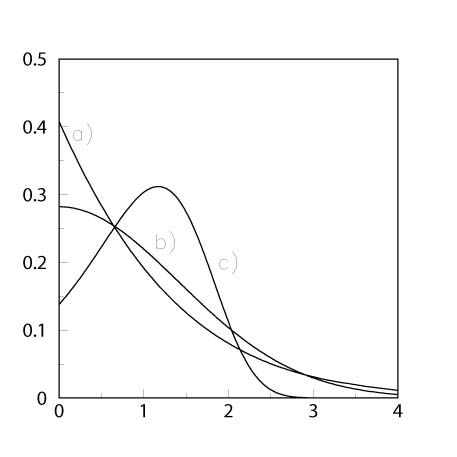
Figure 1: The Cauchy problem for the time-fractional diffusion-wave equation: the fundamental solutions versus $|x|$ with a) $\nu=1/4\,,\;$ b) $\nu=1/2\,,\;$ c) $\nu=3/4\,.$

In Figure 1, as an example we compare versus $|x|\,,$ at fixed $t\,,$ the fundamental solutions of the Cauchy problem with different $\nu$ ($\nu=1/4\,,\,1/2\,,3/4\,$). We consider the range $0\leq|x|\leq 4$ for $t=1$, assuming $a=1$.

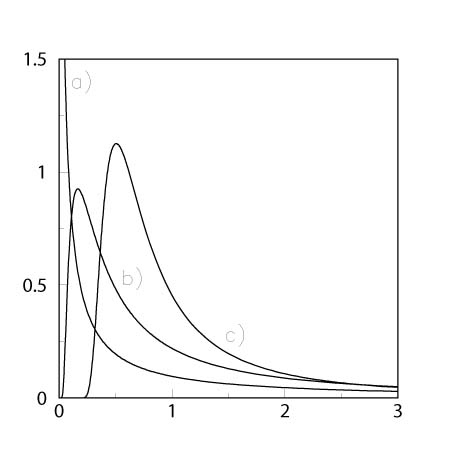
Figure 2: The Signalling problem for the time-fractional diffusion-wave equation: the fundamental solutions versus $t$ with a) $\nu=1/4\,,\;$ b) $\nu=1/2\,,\;$ c) $\nu=3/4\,.$

In Figure 2, as an example we compare versus $t\,,$ at fixed $x\,,$ the fundamental solutions of the Signalling problem with different $\nu$ ($\nu=1/4\,,\,1/2\,,3/4\,$). We consider the range $0\leq t\leq 3$ for $x=1$, assuming $a=1$.

In the limiting cases $\nu=0$ ($\beta=0$) and $\nu=1$ ($\beta=2$) we have

$$\begin{cases}{\displaystyle{\cal{G}}_{c}(x,t;0)}={\displaystyle{{{\rm e}}^{\,\displaystyle-|x|}\over 2}},&\nu=0;\\ {\displaystyle{\cal{G}}_{c}(x,t;1)}={\displaystyle{\delta(x-\sqrt{a}\,t)+\delta(x+\sqrt{a}\,t)\over 2}},&\nu=1.\\ \end{cases}$$

In the limiting cases $\nu=0$ ($\beta=0$) and $\nu=1$ ($\beta=2$) we have

$${\cal{G}}_{s}(x,t;0)=\delta(t)\,,\qquad{\cal{G}}_{s}(x,t;1)=\delta(t-x/\sqrt{a})\,.$$

As outlined at the end of Section 2, in order to ensure a sufficiently low value (of seismological interest) for the constant internal friction $Q^{-1}$, we would inspect the evolution of the initial (seismic) pulses ${\cal{G}}_{c}(x,t;\nu)$ versus $x$ and ${\cal{G}}_{s}(x,t;\nu)$ versus $t$ when the exponent $\gamma$ in the creep power law (2.14) is close to $0$ (nearly elastic cases). In these limiting cases the order $\beta$ of the fractional time derivative tends to 2 from below, since $\beta=2-\gamma$ from (2.13), and our exponent $\nu=\beta/2$ tends to $1$ from above.

For the analysis of the limits the reader is referred to Mainardi & Tomirotti (1997) who have considered the evolution of the seismic pulse for $\nu=1-\delta$ ($\delta=\gamma/2$) taking $\delta=0.001,0.01$.

In these nearly elastic cases the evaluation of the Green functions is indeed‘a difficult task because the matching between their series and saddle point representations is no longer achieved due to the fact that the saddle point turns out to be wide and the consequent approximation becomes poor.

5 The fundamental solutions as probability
density functions

Cauchy Problem: The fundamental solution is provided by the Gauss or normal probability density, symmetric in space.

   $${{\cal{G}}_{c}^{d}(x,t)={1\over 2\sqrt{\pi\,a\,t}}\,{\rm e}^{-\displaystyle x^{2}/(4\,a\,t)}=p_{G}(x;\sigma)\,,}$$   

where

$$p_{G}(x;\sigma):={1\over\sqrt{2\pi}\,\sigma}\,{\rm e}^{\,\displaystyle-x^{2}/(2\sigma^{2})}\,,\;\sigma^{2}=2\,a\,t\,.$$

$$\begin{array}[]{ll}{\cal{P}}_{G}(x;\sigma)&:={\displaystyle\int_{-\infty}^{x}p_{G}(x;\sigma)\,dx={{1\over{2}}}\left[1+{\rm erf}\left({x\over\sqrt{2}\,\sigma}\right)\right]}\\ &={\displaystyle{{1\over{2}}}\left[1+{\rm erf}\left({x\over\sqrt{2at}}\right)\right]}\,.\end{array}$$

$$\begin{array}[]{ll}{\displaystyle\int_{-\infty}^{+\infty}x^{2n}\,p_{G}(x;\sigma)\,dx}&={\displaystyle{(2n)!\over 2^{n}\,n!}\,\sigma^{2n}}\\ &={\displaystyle(2n-1)!!\,\sigma^{2n}=(2n-1)!!\,(2\,a\,t)^{n}}\,.\end{array}$$

Signalling Problem: The fundamental solution is provided by the Lévy-Smirnov probability density, unilateral in time (a property not so well-known as that for the Cauchy problem!).

   $${{\cal{G}}_{s}^{d}(x,t)={x\over 2\sqrt{\pi\,a}\,t^{3/2}}{\rm e}^{-\displaystyle x^{2}/(4\,a\,t)}=p_{LS}(t;\mu)\,,}$$   

$$p_{LS}(t;\mu)={\sqrt{\mu}\over\sqrt{2\pi}\,t^{3/2}}\,{\rm e}^{\,\displaystyle-\mu/(2t)}\,,\;\mu={x^{2}\over 2\,a}\,,$$

$$\begin{array}[]{ll}{{\cal{P}}}_{LS}(t;\mu)&:={\displaystyle\int_{0}^{t}p_{L}(t;\mu)\,dt={\rm erfc}\,\left(\sqrt{{\mu\over 2t}}\right)}\\ &={{\displaystyle\rm erfc}\,\left({x\over 2\,\sqrt{a\,t}}\right)}\,.\end{array}$$

The Lévy-Smirnov $pdf$ has all moments of integer order infinite, since it decays at infinity like $t^{-3/2}$. However, we note that the moments of real order $\delta$ are finite only if $0\leq\delta<1/2\,.$ In particular, for this $pdf$ the mean (expectation) is infinite, but the median is finite. In fact, from ${{\cal{P}}}_{LS}(t_{med};\mu)=1/2\,,$ it turns out that $t_{med}\approx 2\mu\,.$

The Gauss and Lévy–Smirnov laws are special cases of the important class of $\alpha$ - stable probability distributions, or Lévy stable distributions with index of stability (or characteristic exponent) $\alpha=2$ and $\alpha=1/2\,,$ respectively.

Another special case is provided for $\alpha=1$ by the Cauchy-Lorentz law with $pdf$

$$p_{CL}(x;\lambda)={1\over{\pi}}\frac{\lambda}{x^{2}+\lambda^{2}}\,,$$

$$\begin{array}[]{ll}{\cal{P}}_{CL}(x;\mu)&:={\displaystyle\int_{-\infty}^{x}p_{CL}(x;\mu)\,dx}\\ &={\displaystyle{1\over{\pi}}\,{\rm arctang}\left(\frac{x}{\lambda}\right)+\frac{1}{2}}\,.\end{array}$$

The name stable has been assigned to these distributions because of the following property: if two independent real random variables with the same shape or type of distribution are combined linearly and the distribution of the resulting random variable has the same shape, the common distribution (or its type, more precisely) is said to be stable.

More precisely, if $Y_{1}$ and $Y_{2}$ are random variables having such distribution, then $Y$ defined by the linear combination $c\,Y=c_{1}\,Y_{1}+c_{2}\,Y_{2}$ has a similar distribution with the same index $\alpha$ for any positive real values of the constants $c\,,\,c_{1}$ and $c_{2}$ with $c^{\alpha}=c_{1}^{\alpha}+c_{2}^{\alpha}\,.$ As a matter of fact only the range $0<\alpha\leq 2$ is allowed for the index of stability. The case $\alpha=2$ is noteworthy since it corresponds to the normal distribution, which is the only stable distribution which has finite variance, indeed finite moments of any order. In the cases $0<\alpha<2$ the corresponding $pdf$ $p_{\alpha}(y)$ have inverse power tails, i.e. $\int_{|y|>\lambda}p_{\alpha}(y)\,dy=O(\lambda^{-\alpha})\,$ and therefore their absolute moments of order $\delta$ are finite if $0\leq\delta<\alpha$ and infinite if $\delta\geq\alpha\,.$

The inspiration for systematic research on stable distributions, originated with Paul Lévy, was the desire to generalize the celebrated Central Limit Theorem ($CLT$).

The restrictive condition of stability enabled some authors to derive the general form for the characteristic function ($cf$, the Fourier transform of the $pdf$) of a stable distribution, see Feller (1971).

A stable $cf$ is also infinitely divisible, i.e. for every positive integer $n$ it can be expressed as the $n$th power of some $cf$. Equivalently we can say that for every positive integer $n$ a stable $pdf$ can be expressed as the $n$-fold convolution of some $pdf\,.$

All stable $pdf$ are $unimodal$ and indeed bell-shaped, i.e. their $n$-th derivative has exactly $n$ zeros,

The $\alpha$-stable distributions turn out to depend on an additional parameter $\theta$, the skewness parameter. Denoting a stable $pdf$ by $p_{\alpha}(y;\theta)\,,$ we note $p_{\alpha}(-y;-\theta)=p_{\alpha}(y;\theta)\,.$ Consequently a stable $pdf$ with $\theta=0\,$ is necessarily symmetrical. As a matter of fact $|\theta|\leq\alpha$ if $0<\alpha<1$ and $|\theta|\leq 2-\alpha\,$ if $1<\alpha<2\,,$ so the allowed region for $\alpha$ and $\theta$ is the Feller-Takayasu diamond, see Fig. 3.

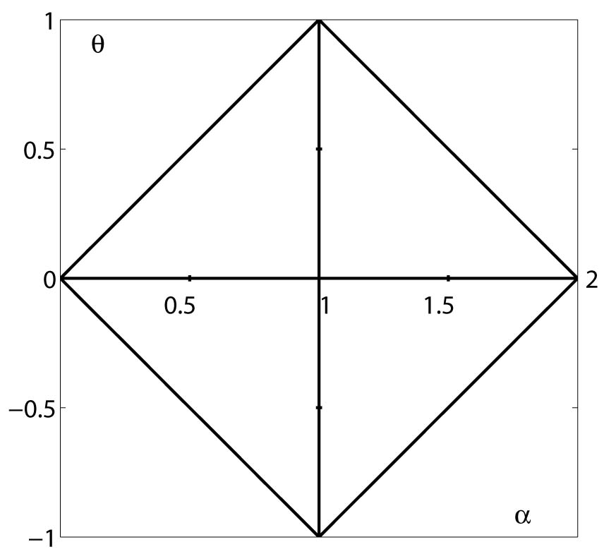
Figure 3: The Feller-Takayasu diamond

One recognizes that the normal distribution is the only stable $pdf$ independent on $\theta$, and that all the extremal stable distributions with $0<\alpha<1$ are unilateral, i.e. vanishing in $\vbox{\hbox to8.9pt{I\hskip-2.1ptR\hfil}}^{\pm}$ if $\theta=\pm\alpha\,.$

In particular, the following representations by convergent power series are valid for stable distributions with $0<\alpha<1$ (negative powers) and $1<\alpha<2$ (positive powers), for $y>0\,:$

$0<\alpha<1\,:$

   $${p_{\alpha}(y;\theta)={1\over\pi\,y}\sum_{n=1}^{\infty}(-y^{-\alpha})^{n}{\Gamma(n\alpha+1)\over n!}\sin\left[{n\pi\over 2}(\theta-\alpha)\right];}$$   

$1<\alpha<2\,:$

   $${p_{\alpha}(y;\theta)={1\over\pi\,y}\sum_{n=1}^{\infty}(-y)^{n}{\Gamma(n/\alpha+1)\over n!}\sin\left[{n\pi\over 2\alpha}(\theta-\alpha)\right].}$$   

In the limiting case $\alpha=2$ ($\theta=0$) we recover the Gauss density (5.2) with $x=y$, $\sigma^{2}=2$. For $\alpha=1$ and $\theta=0$ we recover the Cauchy-Lorentz density (5.8) with $x=y$, $\lambda=1$, whereas for $\alpha=1$ and $\theta=\mp 1$ the singular densities $\delta(y\mp 1)$, see Mainardi, Luchko & Pagnini (2001).

From Eqs. (5.10)-(5.11) a relation between stable $pdf$ with index $\alpha$ and $1/\alpha\,$ can be derived. Assuming $1/2<\alpha<1$ and $y>0\,,$ we obtain

$${1\over{y^{\alpha+1}}}\,p_{1/\alpha}(y^{-\alpha};\theta)=p_{\alpha}(y;\theta^{*})\,,\;\theta^{*}=\alpha(\theta+1)-1\,.$$

A quick check shows that $\theta^{*}$ falls within the prescribed range,

$$|\theta^{*}|\leq\alpha\,,$$

provided that

$$|\theta|\leq 2-1/\alpha\,.$$

Furthermore, we can derive a relation between extremal stable $pdf$ and our auxiliary functions of Wright type. In fact, by comparing (5.10)-(5.11) with the series representations in (3.16)-(3.16) and using (3.19), we obtain

for $0<\alpha<1\,,$

$$p_{\alpha}(y;-\alpha)={1\over{y}}\,F_{\alpha}(y^{-\alpha})={\alpha\over y^{\alpha+1}}\,M_{\alpha}(y^{-\alpha})\,,$$

for $1<\alpha<2\,,$

$$p_{\alpha}(y;\alpha-2)={1\over{y}}\,F_{1/\alpha}(y)={1\over\alpha}\,M_{1/\alpha}(y;)\,.$$

Consequently we can interpret the fundamental solutions (4.1a) and (4.1b) in terms of stable $pdf$, so generalizing the arguments for the standard diffusion equation based on (5.1)-(5.7).

We easily recognize that for $0<\nu<1$ the fundamental solution for the Signalling problem provides a unilateral extremal stable $pdf$ in (scaled) time with index of stability $\alpha=\nu\,,$ which decays according to (4.3b) with a power law.

In fact, from (4.1b) and (5.11) we note that, putting $y=r^{-1/\nu}=\tau=t\,({\sqrt{a}/x})^{1/\nu}>0\,,$

$$(x/\sqrt{a})^{1/\nu}\,{\cal{G}}_{s}(x,t;\nu)=p_{\nu}(\tau;-\nu)\,.$$

This property has been noted also by Kreiss and Pipkin (1986) based on (3.8) and on Feller’s result, $\,p_{\alpha}(t;-\alpha)\div{\rm exp}(-s^{\alpha})$ for $0<\alpha<1\,.$

As far as the Cauchy problem is concerned, we note that the corresponding fundamental solution provides a symmetrical $pdf$ in (scaled) distance with two branches, for $x>0$ and $x<0\,,$ obtained one from the other by reflection. For large $|x|$ each branch exhibits an exponential decay according to (4.3) and, only for $1/2\leq\nu<1\,,$ it is the corresponding branch of an extremal stable $pdf$ with index of stability $\alpha=1/\nu\,.$ In fact, from (4.1b) and (5.14) we note that, putting $y=|r|=\xi=|x|/(\sqrt{a}\,t^{\nu})>0\,,$

$$2\nu\,\sqrt{a}\,t^{\nu}\,{\cal{G}}_{c}(|x|,t;\nu)=p_{1/\nu}(\xi,1/\nu-2)\,.$$

This property had to the author’s knowledge not been noted: it properly generalizes the Gaussian property of the $pdf$ found for $\nu=1/2\,$ (standard diffusion). Furthermore, using (3.22), the moments (of even order) of ${\cal{G}}_{c}(x,t;\nu)$ turn out to be for $n=1\,,\,2\,,\,\dots$:

$$\int_{-\infty}^{+\infty}\!\!\!x^{2n}\,{\cal{G}}_{c}(x,t;\nu)\,dx={\Gamma(2n+1)\over\Gamma(2\nu n+1)}\,(at^{2\nu})^{n}\,.$$

Appendix A. The time fractional derivatives

For a sufficiently well-behaved function $f(t)$ ($t\in\vbox{\hbox to8.9pt{I\hskip-2.1ptR\hfil}}^{+}$) and for any positive number $\mu$ we may define the fractional derivative in two different senses, that we refer here as to Riemann-Liouville derivative and Caputo derivative, respectively. Both derivatives are related to the Riemann-Liouville fractional integral of order $\mu>0$, defined as

   $${J_{t}^{\mu}\,f(t):={1\over{\Gamma(\mu)}}\,\int_{0}^{t}(t-\tau)^{\mu-1}\,f(\tau)\,d\tau\,.}$$   

We note the convention $J_{t}^{0}=I$ (Identity) and the semigroup property for any $\mu,\nu>0$,

$$J_{t}^{\mu}\,J_{t}^{\nu}=\,J_{t}^{\nu}\,J_{t}^{\mu}=J_{t}^{\mu+\nu}\,.$$

The fractional derivative of order $\mu>0$ in the Riemann-Liouville sense is defined as the operator $D_{t}^{\mu}$ which is the left inverse of the Riemann-Liouville integral of order $\mu$ (in analogy with the ordinary derivative), that is

$$D_{t}^{\mu}\,J_{t}^{\mu}=I\,,\;\mu>0\,.$$

If $m$ denotes the positive integer such that $m-1<\mu\leq m\,,$ we recognize from Eqs. (A.2) and (A.3)

$$D_{t}^{\mu}\,f(t):=\,D_{t}^{m}\,J_{t}^{m-\mu}\,f(t)\,,$$

hence for $m-1<\mu<m,$

   $${D_{t}^{\mu}\,f(t)={\displaystyle{d^{m}\over dt^{m}}}\left[{\displaystyle{1\over{\Gamma(m-\mu)}}\int_{0}^{t}{f(\tau)\,d\tau\over(t-\tau)^{\mu+1-m}}}\right]\,,}$$   

and for $\mu=m$

$$D_{t}^{\mu}\,f(t={\displaystyle{d^{m}\over dt^{m}}f(t)}\,.$$

For completion we define $D_{t}^{0}=I\,.$

On the other hand, the fractional derivative of order $\mu>0$ in the Caputo sense is defined as the operator $\,*D_{t}^{\mu}$ such that

$${}_{*}D_{t}^{\mu}\,f(t):=\,_{t}J^{m-\mu}\,_{t}D^{m}\,f(t)\,,$$

hence for $m-1<\mu<m,$

   $${{}_{*}D_{t}^{\mu}\,f(t)={\displaystyle{1\over{\Gamma(m-\mu)}}}\,{\displaystyle\int_{0}^{t}{\displaystyle{f^{(m)}(\tau)\,d\tau\over(t-\tau)^{\mu+1-m}}}}\,,}$$   

and for $\mu=m$

$${}_{*}D_{t}^{m}\,f(t)={\displaystyle{d^{m}\over dt^{m}}f(t)}\,,.$$

This definition requires for non-integer $\mu$ the absolute integrability of the derivative of order $m$. Whenever we use the operator $\,{}_{*}D_{t}^{\mu}$ we (tacitly) assume that this condition is met.

We easily recognize that in general the two fractional derivative differ for non integer orders unless the function $f(t)$ along with its first $m-1$ derivatives vanishes at $t=0^{+}$. In fact, assuming that the passage of the $m$-derivative under the integral is legitimate, we have

   $${D_{t}^{\mu}\,f(t)=\,_{*}D_{t}^{\mu}\,f(t)+\sum_{k=0}^{m-1}f^{(k)}(0^{+})\,\frac{t^{k-\mu}}{\Gamma(k-\mu+1)}\,,}$$   

and therefore, recalling the fractional derivative of the power functions

   $${\,{}_{*}D_{t}^{\mu}\,f(t)=\,D_{t}^{\mu}\left(f(t)-\sum_{k=0}^{m-1}f^{(k)}(0^{+})\,\frac{t^{k}}{k!}\right)\,.}$$   

From (A.7) we recognize that the Caputo fractional derivative represents a sort of regularization in the time origin for the Riemann-Liouville fractional derivative.

We also note that for its existence all the limiting values $f^{(k)}(0^{+}):={\displaystyle\lim_{t\to 0^{+}}\,D_{t}^{k}f(t)}$ are required to be finite for $k=0,1,\dots m-1$.

In the special case $f^{(k)}(0^{+})=0$ for $k=0,1,\dots m-1$, we recover the identity between the two fractional derivatives.

Furthermore we observe that the semigroup property of the standard derivatives is not generally valid for both the fractional derivatives when the order is not integer.

We now explore the most relevant differences between the two fractional derivatives. We first observe their different behaviour at the end points of the interval $(m-1,m)$, namely when the order is any positive integer, as it can be noted from their definitions (A.4), (A.5). For $\mu\to m^{-}$ both derivatives reduce to $\,D_{t}^{m}$, as explicitly stated in Eqs. (A.4b), (A.5b), due to the fact that the operator $\,J_{t}^{0}=\,I$ commutes with $\,D_{t}^{m}$. However, for $\mu\to(m-1)^{+}$ we have:

$$\begin{cases}{\displaystyle\,D_{t}^{\mu}f(t)}\to{\displaystyle D_{t}^{m}\,J_{t}^{1}\,f(t)=D_{t}^{m-1}\,f(t)=f^{(m-1}(t)}\,,\\ {\,{}_{*}D_{t}^{\mu}f(t)}\to{\displaystyle J_{t}^{1}\,D_{t}^{m}\,f(t)=f^{(m-1)}(t)-f^{(m-1)}(0^{+})}\,.\end{cases}$$

As a consequence, roughly speaking, we can say that $\,D_{t}^{\mu}$ is, with respect to its order $\mu\,,$ an operator continuous at any positive integer, whereas $\,{}_{*}D_{t}^{\mu}$ is an operator only left-continuous.

We point out the major utility of the Caputo fractional derivative in treating initial-value problems for physical and engineering applications where initial conditions are usually expressed in terms of integer-order derivatives. This can be easily seen using the Laplace transformation. For the Caputo derivative of order $\mu$ with $m-1<\mu\leq m$ we have

$$\begin{array}[]{ll}\!\!{\cal L}&\left\{\,{}_{*}D_{t}^{\mu}\,f(t);s\right\}\!=\!s^{\mu}\,\widetilde{f}(s)-{\displaystyle\sum_{k=0}^{m-1}s^{\mu-1-k}\,f^{(k)}(0^{+})}\,,\\ &f^{(k)}(0^{+}):={\displaystyle\lim_{t\to 0^{+}}\,D_{t}^{k}f(t)\,.}\end{array}$$

The corresponding rule for the Riemann-Liouville derivative of order $\mu$ is

$$\begin{array}[]{ll}\!\!{\cal L}&\left\{\,D_{t}^{\mu}\,f(t);s\right\}\!=\!s^{\mu}\,\widetilde{f}(s)-{\displaystyle\sum_{k=0}^{m-1}s^{m-1-k}\,g^{(k)}(0^{+})}\,,\\ &g^{(k)}(0^{+}):={\displaystyle\lim_{t\to 0^{+}}\,D_{t}^{k}g(t)\,,}\;{\displaystyle g(t):=\,J_{t}^{m-\mu}\,f(t)\,.}\end{array}$$

Thus the rule (A.10) is more cumbersome to be used than (A.9) since it requires initial values concerning an extra function $g(t)$ related to the given $f(t)$. However, when all the limiting values $f^{(k)}(0^{+})$ are finite and the order is not integer, we can prove by that all $g^{(k)}(0^{+})$ vanish so that the formula (A.10) simplifies into

$${\cal L}\left\{D_{t}^{\mu}\,f(t);s\right\}=s^{\mu}\,\widetilde{f}(s)\,,\;m-1<\mu<m\,.$$

In the special case $f^{(k)}(0^{+})=0$ for $k=0,1,m-1$, we recover the identity between the two fractional derivatives.

We note that the Laplace transform rule (A.9) was the starting point of Caputo, see Caputo (1967), Caputo (1969), for defining his generalized derivative in the late sixties.

Appendix B. The plots of the M-Wright function

To gain more insight of the effect of the parameter $\nu$ on the behaviour of the $M_{\nu}$ Wright function close to and far from the origin, we will adopt both linear and logarithmic scale for the ordinates. In Figs. B.1 and B.2 we compare the plots of the $M_{\nu}(|x|)$-Wright functions in $|x|\leq 5$ for some rational values in the ranges $\nu\in[0,1/2]$ and $\nu\in[1/2,1]$, respectively. Thus in Fig. B.1 we see the transition from $\exp(-|x|)$ for $\nu=0$ to $1/\sqrt{\pi}\,\exp(-x^{2})$ for $\nu=1/2$, whereas in Fig. B.2 we see the transition from $1/\sqrt{\pi}\,\exp(-x^{2})$ for $\nu=1/2$ to the delta functions $\delta(x\pm 1)$ for $\nu=1$.

Fig. B1 - Plots of $M_{\nu}(|x|)$ with $\nu=0,1/8,1/4,3/8,1/2$ for $|x|\leq 5$;

top: linear scale, bottom: logarithmic scale.

Fig. B2 - Plots of $M_{\nu}(|x|)$ with $\nu=1/2\,,\,5/8\,,\,3/4\,,\,1$ for $|x|\leq 5$:

top: linear scale; bottom: logarithmic scale)

In plotting $M_{\nu}(|x|)$ at fixed $\nu$ for sufficiently large $|x|$ the asymptotic representation (3.20) is useful since, as $|x|$ increases, the numerical convergence of the series in (3.17) becomes poor and poor up to being completely inefficient.

However, as $\nu\to 1^{-}$, the plotting remains a very difficult task because of the high peaks arising around $x=\pm 1$.

In Fig. B.3 we consider the cases $\nu=1-\epsilon$: (a) $\epsilon=0.01\,,$ (b) $\epsilon=0.001\,.$ Here the plots are obtained by the method of Kreis & Pipkin [28] (continuous line), by adding 100 terms-series (dashed line) and by the standard saddle-point method (dashed-dotted line).

Fig. B3 - Plots of $M_{\nu}(x)$ with $\nu=1-\epsilon$ around the maximum $x\approx 1$;

left: (a) $\epsilon=0.01\,,$ right: (b) $\epsilon=0.001$.

References

- [1] Buchen, P.W. and Mainardi, F. (1975): Asymptotic expansions for transient viscoelastic waves, Journal de Mécanique 14, 597-608.
- [2] Caputo, M. (1966): Linear models of dissipation whose Q is almost frequency independent, Annali di Geofisica 19, 383-393.
- [3] Caputo, M. (1967): Linear models of dissipation whose Q is almost frequency independent, Part II., Geophys. J. R. Astr. Soc. 13, 529-539. [Reprinted in: Fractional Calculus and Applied Analysis 11 (2008), No 1, 3-14.]
- [4] Caputo, M. (1969): Elasticità e Dissipazione (Zanichelli Bologna). [in Italian]
- [5] Caputo, M. and Mainardi, F. (1971a): A new dissipation model based on memory mechanism, Pure and Applied Geophysics (Pageoph) 91, 134-147. [Reprinted in: Fractional Calculus and Applied Analysis 10 (2007), No 3, 309-324.]
- [6] Caputo, M. and Mainardi, F. (1971b): Linear models of dissipation in anelastic solids, Rivista del Nuovo Cimento (Ser II) 1, 161-198.
- [7] Caputo, M. (1973): Elasticity with dissipation represented by a simple memory mechanism, Atti Accad. Naz. Lincei, Rend. Classe Scienze (Ser. 8), 55, 467-470.
- [8] Caputo, M. (1976): Vibrations of an infinite plate with a frequency independent J. Acoust. Soc. Am. 60, 634-639.
- [9] Caputo, M. (1979): A model for the fatigue in elastic materials with frequency independent J. Acoust. Soc. Am. 66, 176-179.
- [10] Caputo, M. (1996): The Green function of the diffusion in porous media with memory, Rend. Fis. Acc. Lincei (Ser. 9) 7, 243-250.
- [11] Chin, R.C.Y. (1980): Wave propagation in viscoelastic media, in Physics of the Earth’s Interior, edited by A. Dziewonski and E. Boschi (North-Holland, Amsterdam), pp. 213-246. [E. Fermi Int. School, Course 78]
- [12] Christensen, R.M. (1982): Theory of Viscoelasticity (Academic Press, New York). [1-st ed. (1972)]
- [13] Dzherbashyan, M.M. and Nersesyan, A.B. (1968): Fractional derivatives and the Cauchy problem for differential equations of fractional order. Izv. Acad. Nauk Armjanskvy SSR, Matematika 3, 3–29. [In Russian]
- [14] Engler, H. (1997): Similarity solutions for a class of hyperbolic integro-differential equations, Differential Integral Equations 10, 815-840.
- [15] Erdélyi, A. Editor (1955): Higher Transcendental Functions, Bateman Project (McGraw-Hill, New York), Vol. 3, Ch. 18, pp. 206-227.
- [16] Feller, W. (1971): An Introduction to Probability Theory and its Applications, (Wiley, New York), Vol. II, Ch. 6: pp. 169-176, Ch. 13: pp. 448-454. [1-st ed. (1966)]
- [17] Fujita, Y. (1990a): Integro-differential equation which interpolates the heat equation and the wave equation, I, II, Osaka J. Math. 27, 309-321, 797-804.
- [18] Fujita, Y. (1990b): Cauchy problems of fractional order and stable processes, Japan J. Appl. Math. 7, 459-476.
- [19] Giona, M. and Roman, H.E. (1992): Fractional diffusion equation for transport phenomena in random media, Physica A 185, 82-97.
- [20] Gonsovskii, V.L. and Rossikhin, Yu.A. (1973): Stress waves in a viscoelastic medium with a singular hereditary kernel, Zhurnal Prikladnoi Mekhaniki Tekhnicheskoi Fiziki 4, 184-186. [Translated from the Russian by Plenum Publishing Corporation, New York (1975)]
- [21] Gorenflo, R., Iskenderov, A. and Luchko, Yu. (2000): Mapping between solutions of fractional diffusion-wave equations, Fractional Calculus and Applied Analysis 3, 75-86.
- [22] Gorenflo, R. and Mainardi, F. (1997): Fractional calculus: integral and differential equations of fractional order, in Fractals and Fractional Calculus in Continuum Mechanics, edited by A. Carpinteri and F. Mainardi (Springer Verlag, Wien), 223-276.
- [23] Graffi, D. (1982): Mathematical models and waves in linear viscoelasticity, in Wave Propagation in Viscoelastic Media, edited by F. Mainardi (Pitman, London), pp. 1-27. [Res. Notes in Maths, Vol. 52]
- [24] Hunter, S.C. (1960): Viscoelastic Waves, in Progress in Solid Mechanics, edited by I. Sneddon and R. Hill (North-Holland, Amsterdam), Vol 1, pp. 3-60.
- [25] Kilbas, A.A., Srivastava, H.M. and Trujillo, J.J. (2006): Theory and Applications of Fractional Differential Equations, (Elsevier, Amsterdam). [North-Holland Mathematics Studies No 204]
- [26] Kochubei, A.N. (1990): Fractional-order diffusion, Differential Equations 26, 485-492. [English translation from the Russian Journal Differenttsial’nye Uravneniya]
- [27] Kolsky, H. (1956): The propagation of stress pulses in viscoelastic solids, Phil. Mag. (Ser 8) 2, 693-710.
- [28] Kreis, A. and Pipkin, A.C. (1986): Viscoelastic pulse propagation and stable probability distributions, Quart. Appl. Math. 44, 353-360.
- [29] Mainardi, F. (1994): On the initial value problem for the fractional diffusion-wave equation, in Waves and Stability in Continuous Media edited by S. Rionero and T. Ruggeri, (World Scientific, Singapore), pp. 246-251.
- [30] Mainardi, F. (1995): Fractional diffusive waves in viscoelastic solids in IUTAM Symposium - Nonlinear Waves in Solids, edited by J. L. Wegner and F. R. Norwood (ASME/AMR, Fairfield NJ), pp. 93-97. [Abstract in Appl. Mech. Rev. 46 (1993), 549]
- [31] Mainardi, F. (1996a): Fractional relaxation-oscillation and fractional diffusion-wave phenomena, Chaos, Solitons & Fractals 7, 1461-1477.
- [32] Mainardi, F. (1996b): The fundamental solutions for the fractional diffusion-wave equation, Applied Mathematics Letters 9, No 6, 23-28.
- [33] Mainardi, F. (1997): Fractional calculus; some basic problems in continuum and statistical mechanics, in Fractals and Fractional Calculus in Continuum Mechanics, edited by. A. Carpinteri and F. Mainardi (Springer-Verlag, Wien), 291-348.
- [34] Mainardi, F. (2002a) : Linear viscoelasticity, Chapter 4 in: A. Guran, A. Boström, O. Leroy and G. Maze (Editors), Acoustic Interactions with Submerged Elastic Structures, Part IV: Nondestructive Testing, Acoustic Wave Propagation and Scattering, (World Scientific, Singapore), pp. 97-126. [Vol. 5 on the Series B on Stability, Vibration and Control of Systems]
- [35] Mainardi, F. (2002b): Transient waves in linear viscoelastic media, Chapter 5 in: A. Guran, A. Boström, O. Leroy and G. Maze (Editors), Acoustic Interactions with Submerged Elastic Structures, Part IV: Nondestructive Testing, Acoustic Wave Propagation and Scattering, (World Scientific, Singapore), pp. 127-161.
- [36] Mainardi, F. (2008): Fractional Calculus and Waves in Linear Viscoelasticity (Imperial College Press, London), in preparation.
- [37] Mainardi, F. and Gorenflo, R. (2007): Time-fractional derivatives in relaxation processes: a tutorial survey, Fractional Calculus and Applied Analysis 10, 269-308. [E-print http://arxiv.org/abs/0801.4914]
- [38] Mainardi, F. Luchko, Yu. and Pagnini, G. (2001): The fundamental solution of the space-time fractional diffusion equation, Fractional Calculus and Applied Analysis 4, 153-192. [E-print http://arxiv.org/abs/cond-mat/0702419]
- [39] Mainardi, F. and Pagnini, G. (2003): The Wright functions as solutions of the time-fractional diffusion equations, Applied Mathematics and Computation 141, 51-66.
- [40] Mainardi, F. and Paradisi, P. (2001): Fractional diffusive waves, Journal of Computational Acoustics 9, 1417-1436.
- [41] Mainardi, F. and Tomirotti, M. (1995): On a special function arising in the time fractional diffusion-wave equation, in Transform Methods and Special Functions, Sofia 1994, edited by P. Rusev, I. Dimovski and V. Kiryakova, (Science Culture Technology, Singapore), pp. 171-183.
- [42] Mainardi, F. and Tomirotti, M. (1997): Seismic pulse propagation with constant and stable probability distributions, Annali di Geofisica 40, 1311-1328.
- [43] Mainardi, F. and Turchetti, G. (1975): Wave front expansion for transient viscoelastic waves, Mech. Res. Comm. 2, 107-112.
- [44] Meshkov, S.I. and Rossikhin, Yu. A. (1970): Sound wave propagation in a viscoelastic medium whose hereditary properties are determined by weakly singular kernels, in Waves in Inelastic Media, edited by Yu. N. Rabotnov (Kishniev), pp. 162-172. [in Russian]
- [45] Metzler, R., Glöckle, W.G. and Nonnenmacher, T.F. (1994): Fractional model equation for anomalous diffusion, Physica A 211, 13-24.
- [46] Nigmatullin, R.R. (1986): The realization of the generalized transfer equation in a medium with fractal geometry, Phys. Stat. Sol. B 133, 425-430. [English translation from the Russian]
- [47] Pipkin, A.C. (1986): Lectures on Viscoelastic Theory (Springer-Verlag, New York), Ch. 4, pp. 56-76. [1-st ed, 1972]
- [48] Podlubny, I. (1999): Fractional Differential Equations (Academic Press, San Diego). [Mathematics in Science and Engineering, Vol. 198]
- [49] Prüsse, J. (1993): Evolutionary Integral Equations and Applications, (Birkhauser Verlag, Basel).
- [50] Rabotnov, Yu. N. (1969): Creep Problems in Structural Members, North-Holland, Amsterdam. [English translation of the 1966 Russian edition]
- [51] Rossikhin, Yu. A. and Shitikova, M.V. (1997): Application of fractional calculus to dynamic problems of linear and nonlinear hereditary mechanics of solids, Applied Mechanics Review 50, 15-67.
- [52] Rossikhin, Yu.A. and Shitikova, M.V. (2007). Comparative analysis of viscoelastic models involving fractional derivatives of different orders, Fractional Calculus and Applied Analysis 10 No 2, 111-121.
- [53] Rossikhin, Yu.A. and Shitikova, M.V. (2010): Applications of fractional calculus to dynamic problems of solid mechanics: novel trends and recent results, Appl. Mech. Review 63, 010801/1–52.
- [54] Samko S.G., Kilbas, A.A. and O.I. Marichev (1993): Fractional Integrals and Derivatives, Theory and Applications, (Gordon and Breach, Amsterdam).
- [55] Schneider, W.R. and Wyss, W. (1989): Fractional diffusion and wave equations, J. Math. Phys. 30, 134-144.
- [56] Scott-Blair, G.W. (1949): Survey of General and Applied Rheology, Pitman, London.
- [57] Strick, E. (1970): A predicted pedestal effect for pulse propagation in constant- solids, Geophysics 35, 387-403.
- [58] Strick, E. (1982): Application of linear viscoelasticity to seismic wave propagation, in Wave Propagation in Viscoelastic Media, edited by F. Mainardi (Pitman, London), pp. 169-193. [Res. Notes in Maths, Vol. 52]
- [59] Strick, E. and Mainardi, F. (1982): On a general class of constant solids, Geophys. J. R. Astr. Soc. 69, 415-429
- [60] Uchaikin, V.V. and Zolotarev, V.M. (1999): Chance and Stability. Stable Distributions and their Applications, VSP, Utrecht.