Performance of local orbital basis sets in the self-consistent Sternheimer method for dielectric matrices of extended systems

Abstract

We present a systematic study of the performance of numerical pseudo-atomic orbital basis sets in the calculation of dielectric matrices of extended systems using the self-consistent Sternheimer approach of [F. Giustino et al., Phys. Rev. B 81(11), 115105 (2010)]. In order to cover a range of systems, from more insulating to more metallic character, we discuss results for the three semiconductors diamond, silicon, and germanium. Dielectric matrices calculated using our method fall within 1-3% of reference planewaves calculations, demonstrating that this method is promising. We find that polarization orbitals are critical for achieving good agreement with planewaves calculations, and that only a few additional $\zeta$’s are required for obtaining converged results, provided the split norm is properly optimized. Our present work establishes the validity of local orbital basis sets and the self-consistent Sternheimer approach for the calculation of dielectric matrices in extended systems, and prepares the ground for future studies of electronic excitations using these methods.

I Introduction

In recent years electronic structure codes based on local orbital basis sets have proven successful in describing complex systems involving several thousands of atoms.Soler et al. (2002); Skylaris et al. (2005); Bowler and Miyazaki (2010) The key concept behind the use of local orbital basis sets in the solid state is that the ground-state electronic density matrix is exponentially localized in insulators.Kohn (1996) As a consequence of this localization, the representation of one-particle operators in a local orbital basis leads to strictly sparse matrices. It is therefore possible to solve the electronic structure problem, e.g. the Kohn-Sham equations of density-functional theory (DFT), using numerical methods whose complexity scales linearly as a function of system size.Ordejón et al. (1993); Mauri et al. (1993); Ordejón et al. (1996); Goedecker (1999)

A natural question arising is whether such local orbital basis sets would also be advantageous in the study of electronic excitations. Since these basis sets are optimized for providing an accurate description of ground-state properties, it is not clear a priori how to exploit them for calculating excited state properties. For example, in the specific case of $GW$ calculationsHedin (1965); Hybertsen and Louie (1986) the Green’s function and the screened Coulomb interaction are both evaluated by using expansions over unoccupied electronic states. However, local orbital basis sets typically provide a poor description of unoccupied states, and the convergence as a function of basis size is not systematic as in the case of planewaves basis setsIhm et al. (1979) or finite difference methods.Chelikowsky et al. (1994) In this context it would be desirable to develop new methods for electronic excitations which (i) retain the favorable scaling of local orbital basis sets, and (ii) do not require the explicit calculation of unoccupied states.

Recently several schemes have been proposed in order to reduce or avoid the evaluation of unoccupied states in excited-state calculations.Bruneval and Gonze (2008); Berger et al. (2010); Wilson et al. (2008, 2009); Giustino et al. (2010); Umari et al. (2010) In Refs. Bruneval and Gonze, 2008; Berger et al., 2010 a small number of unoccupied states or even one single state are used to effectively replace the expansion over the conduction manifold. The authors of Ref. Wilson et al., 2008, 2009 use selected eigenvectors of the dielectric matrix in order to evaluate the screened Coulomb interaction without explicitly performing sums over empty states. In Ref. Umari et al., 2010 a Lanczos algorithm is used in order to calculate the dielectric matrix using continued fractions, without performing sums over empty states.

We here consider the scheme proposed in Ref. Giustino et al., 2010 for evaluating the screened Coulomb interaction in extended systems. In this scheme the expansion over unoccupied states and the matrix inversion are avoided altogether, and replaced by the self-consistent solution of Sternheimer equations. In a recent workHübener et al. (2012) we have extended the scheme of Ref. Giustino et al., 2010 to the case of local orbital basis sets, and implemented our new scheme using the SIESTA package.Soler et al. (2002) Ref. Hübener et al., 2012 represents, to our knowledge, the first implementation of the self-consistent Sternheimer equation in a local orbitals basis for extended systems.

In the present manuscript we complement and extend the work of Ref. Hübener et al., 2012 by systematically comparing the performance of numerical pseudo-atomic orbital basis sets with standard plane-waves results. Since most excited-state calculations involve kernels describing the nonlocal and time-dependent dielectric screening of the material, we here focus on the the frequency- and wavevector- dependent dielectric matrix of representative semiconductors.

The manuscript is organized as follows. In Sec. II we describe our methodology. In particular, in Sec. II.1 we summarize the self-consistent Sternheimer scheme for the screened Coulomb interaction and the inverse dielectric matrix. In Secs. II.2 and II.3 we specialize the formalism to the case of local orbital basis sets and periodic systems, respectively. In Sec. III we briefly describe the basis set of SIESTA that we use in all our calculations (Sec. III.1) and we provide details on the structural and convergence parameters used in the calculations (Sec. III.2). In Sec. IV we discuss our results, focusing on the three semiconductors diamond, silicon, and germanium. This choice allows us to understand how the performance of our methodology varies when moving from more insulating (diamond) to more metallic systems (germanium). In particular we investigate both the static dielectric matrices (Sec. IV.1), and the frequency- and wavevector-dependent dielectric functions (Sec. IV.2). In Sec. V we summarize our findings and draw our conclusions. We leave to Appendix A some technical details of our implementation.

II Theoretical methodology

II.1 Self-consistent Sternheimer approach for the screened Coulomb interaction

The first order change of the valence Kohn-Sham wavefunction $\psi_{\mathnormal{v}}$ due to the perturbation $\Delta V$ is expressed by the Sternheimer equation as:

$$(\hat{H}-\epsilon_{\mathnormal{v}})\Delta\psi_{\mathnormal{v}}=-(1-\hat{P}_{v})\Delta V\psi_{\mathnormal{v}},$$ (1)

where $\hat{H}$ is the Kohn-Sham Hamiltonian and $1-\hat{P}_{v}$ is the projector on the conduction manifold. The corresponding change in the valence electron density is given by:

$$\Delta n=4{\rm Re}\sum_{\mathnormal{v}}\psi_{\mathnormal{v}}^{*}\Delta\psi_{\mathnormal{v}},$$ (2)

where the prefactor also takes into account the spin degeneracy (we refer to spin-unpolarized systems for simplicity). The density variation of Eq. (2) induces a change in the self-consistent potential $\Delta V$ experienced by the electrons (through the Hartree and exchange-correlation terms), therefore Eqs. (1) and (2) must be solved iteratively. This procedure is at the core of density-functional perturbation theory for lattice dynamics.Baroni et al. (1987, 2001)

In the following we summarize the extension of the self-consistent Sternheimer approach to the calculation of the screened Coulomb interaction $W$ and the inverse dielectric matrix $\epsilon^{-1}$, as derived in Ref. Giustino et al., 2010. These quantities are both functions of the real-space variables $\mathbf{r}$, $\mathbf{r}^{\prime}$, and of the frequency $\omega$, and are related to the bare Coulomb interaction $v$ through:

$$W(\mathbf{r},\mathbf{r}^{\prime};\omega)=\int d\mathbf{r}^{\prime\prime}\epsilon^{-1}(\mathbf{r},\mathbf{r}^{\prime\prime};\omega)v(\mathbf{r}^{\prime\prime},\mathbf{r}^{\prime}).$$ (3)

The calculation of $\epsilon^{-1}$ starting from $W$ is straightforward in reciprocal space, therefore in the following we focus on the screened Coulomb interaction. We first parametrize the frequency and one spatial variable of $W$ by defining the potential $\Delta V_{[\mathbf{r},\omega]}(\mathbf{r}^{\prime})=W(\mathbf{r},\mathbf{r}^{\prime};\omega)$. This potential induces a change $\Delta\psi^{\pm}_{\mathnormal{v}[\mathbf{r},\omega]}$ of the valence wavefunction $\psi_{\mathnormal{v}}$ given by:

$$(\hat{H}-\epsilon_{\mathnormal{v}}\pm\omega)\Delta\psi^{\pm}_{\mathnormal{v}[\mathbf{r},\omega]}=-(1-\hat{P}_{\mathnormal{v}})\Delta V_{[\mathbf{r},\omega]}\psi_{\mathnormal{v}}.$$ (4)

The associated variation of the density matrix is

$$\Delta n_{[\mathbf{r},\omega]}=2\sum_{\mathnormal{v},\sigma=\pm}\psi^{*}_{\mathnormal{v}}\Delta\psi^{\sigma}_{\mathnormal{v}[\mathbf{r},\omega]}.$$ (5)

In the random-phase approximation (RPA) this variation generates the screening Hartree potential Giustino et al. (2010)

$$\Delta V^{H}_{[\mathbf{r},\omega]}(\mathbf{r}^{\prime})=\int d\mathbf{r}^{\prime\prime}\Delta n_{[\mathbf{r},\omega]}(\mathbf{r}^{\prime\prime})\mathnormal{v}(\mathbf{r}^{\prime\prime},\mathbf{r}^{\prime}),$$ (6)

which is added to the bare Coulomb potential in order to obtain the total self-consistent potential appearing in Eq. (4):

$$\Delta V_{[\mathbf{r},\omega]}(\mathbf{r}^{\prime})=v(\mathbf{r},\mathbf{r}^{\prime})+\Delta V^{H}_{[\mathbf{r},\omega]}(\mathbf{r}^{\prime}).$$ (7)

The iterative self-consistent solution of Eqs. (4)-(7) for all the values of the parameters $\mathbf{r}$ and $\omega$ yields the screened Coulomb interaction $W$. This scheme is exactly equivalentGiustino et al. (2010) to evaluating $W$ via Hedin’s equation

$$W=\mathnormal{v}+WP\mathnormal{v},$$ (8)

$P$ being the RPA polarizability.

II.2 Self-consistent Sternheimer approach with local orbitals

In order to implement the method described in Sec. II.1 within the basis of local orbitals $\phi_{i}(\mathbf{r}^{\prime})$ we expand the wavefunctions and their first order variations as:

$$\psi_{\mathnormal{v}}(\mathbf{r}^{\prime}) = \sum_{i}c_{\mathnormal{v}i}\phi_{i}(\mathbf{r}^{\prime}),$$ (9)

$$\Delta\psi_{\mathnormal{v}[\mathbf{r},\omega]}(\mathbf{r}^{\prime}) = \sum_{i}\Delta c_{\mathnormal{v}i[\mathbf{r},\omega]}\phi_{i}(\mathbf{r}^{\prime}).$$ (10)

The expansions would be exact if the local orbitals were to span the entire Hilbert space of the single-particle Hamiltonian. In practice the representation of the valence wavefunctions is expected to be accurate, while the description of the variations requires some care because they arise from the conduction manifold. By replacing Eqs. (9)-(10) inside Eq. (4) and performing scalar products of both sides with basis functions we obtain the matrix equations:

$$\left[\mathbf{H}-(\epsilon_{\mathnormal{v}}\pm\omega)\mathbf{S}\right]\Delta\mathbf{c}^{\pm}_{\mathnormal{v}[\mathbf{r},\omega]}=-\left[\mathbf{1}-\mathbf{S}\mbox{\boldmath$\rho$}^{T}\right]\Delta\mathbf{V}_{[\mathbf{r},\omega]}\mathbf{c}_{\mathnormal{v}},$$ (11)

where the Hamiltonian $\mathbf{H}$, overlap $\mathbf{S}$, density $\rho$, and perturbation $\Delta\mathbf{V}_{[\mathbf{r},\omega]}$ matrices are defined in the usual notation as:

$$H_{ij} = \langle\phi_{i}|H|\phi_{j}\rangle,$$ (12)

$$S_{ij} = \langle\phi_{i}|\phi_{j}\rangle,$$ (13)

$$\rho_{ij} = \sum_{v^{\prime}}c^{*}_{v^{\prime}i}c_{v^{\prime}j},$$ (14)

$$\Delta V_{ij[\mathbf{r},\omega]} = \langle\phi_{i}|\Delta V_{[\mathbf{r},\omega]}|\phi_{j}\rangle.$$ (15)

The Hamiltonian, the overlap, and the density matrices are readily available in any local orbital DFT implementation. The matrix elements $\Delta V_{ij[\mathbf{r},\omega]}$ require careful consideration. The iterative self-consistent solution of the Sternheimer equation starts with $\Delta V_{[\mathbf{r},\omega]}(\mathbf{r}^{\prime})$ initialized to the bare Coulomb potential $v(\mathbf{r},\mathbf{r}^{\prime})$. This is a nonlocal potential, therefore an expansion in the local orbital basis would require the product functions $\phi_{i}(\mathbf{r})\phi_{j}(\mathbf{r}^{\prime})$.Aryasetiawan and Gunnarsson (1994) Using such expansionRohlfing et al. (1995); Blase and Ordejón (2004); Koval et al. (2010); Foerster et al. (2011); Blase et al. (2011) in Eq. (15) would ultimately lead to the evaluation of four-point integrals, and would also introduce three-point overlaps in the Sternheimer equations. In addition, the validity of such expansion for the Coulomb potential is not guaranteed. In order to avoid this difficulty we evaluate the integral of Eq. (15) in real space. This real-space integral is part of the SIESTA implementation. We stress that the evaluation of Eq. (15) in real space does not suffer from representability issues associated with a product-basis expansion, and we do not make use of the expansion of the identity operator in the local orbital basis.

The solution of Eq. (11) yields the vector $\Delta\bf{c}$ of the linear response coefficients which are used to construct the variation of the density matrix:

$$\Delta n_{ij[\mathbf{r},\omega]}=2\sum_{\mathnormal{v},\sigma=\pm}c^{*}_{\mathnormal{v}i}\Delta c^{\sigma}_{\mathnormal{v}j[\mathbf{r},\omega]}.$$ (16)

For the evaluation of the induced Hartree potential Eq. (6), first the variation of the density matrix is calculated on the real-space grid:

$$\Delta n_{[\mathbf{r},\omega]}(\mathbf{r}^{\prime})=\sum_{ij}\Delta n_{ij[\mathbf{r},\omega]}\phi^{*}_{i}(\mathbf{r}^{\prime})\phi^{*}_{j}(\mathbf{r}^{\prime}),$$ (17)

then standard Fourier-transform techniques are employed. The convergence of the scf-cycle is tested on the variation of the density matrix Eq. (16).

The self-consistent procedure is carried out independently for the parameters $\mathbf{r}$ and $\omega$. Apart from leading to a trivial parallelization, this scheme has the advantage that the parametrized space variable $\mathbf{r}$ can be represented on a coarser grid than the one used for $\mathbf{r}^{\prime}$ and the real-space integrals. Indeed, the accuracy required for operations in $\mathbf{r}^{\prime}$ is the same needed to describe the Kohn-Sham Hamiltonian, while the accuracy for $\mathbf{r}$ is the one needed to represent the screened Coulomb interaction.

II.3 Self-consistent Sternheimer approach with local orbitals for periodic systems

In order to address extended periodic systems and compare our results with calculations based on planewaves basis sets, in this section we specialize the formalism of Sec. II.2 to the case of crystalline solids. We start by introducing a new basis set which satisfies Bloch’s theorem from the outset. For this purpose we define the cell-periodic functions:

$$\phi_{i\mathbf{k}}(\mathbf{r}^{\prime})=\sum_{\mathbf{R}}e^{-i\mathbf{k}\cdot(\mathbf{r}^{\prime}-\mathbf{R})}\phi_{i}(\mathbf{r}^{\prime}-\mathbf{R}),$$ (18)

where $\mathbf{k}$ is a point in the Brillouin zone and $\mathbf{R}$ a lattice vector. In Eq. (18) the orbitals $\phi_{i}(\mathbf{r}^{\prime})$ are the same as in Eq. (9), except that here they only span the unit cell of the crystal. It is immediate to verify that the functions $e^{i\mathbf{k}\cdot\mathbf{r}^{\prime}}\phi_{i\mathbf{k}}(\mathbf{r}^{\prime})$ satisfy Bloch’s theorem, and that the basis functions $\phi_{i\mathbf{k}}$ are periodic.

In analogy with Eqs. (9), (10) we expand the periodic part $u_{\mathnormal{v}\mathbf{k}}$ of the Kohn-Sham eigenfunctions $\psi_{\mathnormal{v}\mathbf{k}}(\mathbf{r}^{\prime})=e^{i\mathbf{k}\cdot\mathbf{r}^{\prime}}u_{\mathnormal{v}\mathbf{k}}(\mathbf{r}^{\prime})$ using the basis $\phi_{i\mathbf{k}}$:

$$u_{v\mathbf{k}}(\mathbf{r}^{\prime}) = \sum_{i}c_{vi\mathbf{k}}\phi_{i\mathbf{k}}(\mathbf{r}^{\prime}),$$ (19)

$$\Delta u_{v\mathbf{k}[\mathbf{q},\mathbf{r}]}(\mathbf{r}^{\prime}) = \sum_{i}\Delta c_{vi\mathbf{k}[\mathbf{q},\mathbf{r}]}\phi_{i\mathbf{k}+\mathbf{q}}(\mathbf{r}^{\prime}).$$ (20)

By rewriting Eq. (4) for a periodic systemGiustino et al. (2010) and taking scalar products with basis functions we obtain the analogue of Eq. (11) for crystalline systems:

$$\begin{split}&\left[\mathbf{H}_{\mathbf{k}+\mathbf{q}}-(\epsilon_{\mathnormal{v}\mathbf{k}}\pm\omega)\mathbf{S}_{\mathbf{k}+\mathbf{q}}\right]\Delta\mathbf{c}^{\pm}_{\mathnormal{v}\mathbf{k}[\mathbf{q},\mathbf{r},\omega]}=\\ &\qquad\qquad\;-\left[\mathbf{1}-\mathbf{S}_{\mathbf{k}+\mathbf{q}}\mbox{\boldmath$\rho$}^{T}_{\mathbf{k}+\mathbf{q}}\right]\Delta\mathbf{V}_{\mathbf{k}[\mathbf{q},\mathbf{r},\omega]}\mathbf{c}_{\mathnormal{v}\mathbf{k}}.\end{split}$$ (21)

In this case the Hamiltonian and the overlap matrices are defined as:

$$H_{ij\mathbf{k}} = \sum_{\mathbf{R}}e^{i\mathbf{k}\cdot\mathbf{R}}\int d\mathbf{r}^{\prime}\phi_{i}(\mathbf{r}^{\prime})H(\mathbf{r}^{\prime})\phi_{j}(\mathbf{r}^{\prime}-\mathbf{R}),$$ (22)

$$S_{ij\mathbf{k}} = \sum_{\mathbf{R}}e^{i\mathbf{k}\cdot\mathbf{R}}\int d\mathbf{r}^{\prime}\phi_{i}(\mathbf{r}^{\prime})\phi_{j}(\mathbf{r}^{\prime}-\mathbf{R}).$$ (23)

The perturbation matrix reads:

$$\Delta V_{ij\mathbf{k}[\mathbf{q},\mathbf{r},\omega]}=\int d\mathbf{r}^{\prime}\phi^{*}_{i\mathbf{k}+\mathbf{q}}(\mathbf{r}^{\prime})\Delta v_{[\mathbf{q},\mathbf{r}]}(\mathbf{r}^{\prime})\phi_{j\mathbf{k}}(\mathbf{r}^{\prime})$$

$$=\sum_{\mathbf{R}}e^{i\mathbf{k}\cdot\mathbf{R}}\int d\mathbf{r}^{\prime}\phi_{i}(\mathbf{r}^{\prime})\Delta v_{[\mathbf{q},\mathbf{r}]}(\mathbf{r}^{\prime})e^{i\mathbf{q}\cdot\mathbf{r}^{\prime}}\phi_{j}(\mathbf{r}^{\prime}-\mathbf{R}),$$ (24)

where $\Delta v_{[\mathbf{q},\mathbf{r},\omega]}(\mathbf{r}^{\prime})$ is the cell-periodic component of the perturbation with wavevector $\mathbf{q}$:Giustino et al. (2010)

$$\Delta V_{[\mathbf{r},\omega]}(\mathbf{r}^{\prime})=\frac{1}{N_{\mathbf{q}}}\sum_{\mathbf{q}}e^{i\mathbf{q}\cdot(\mathbf{r}^{\prime}-\mathbf{r})}\Delta v_{[\mathbf{q},\mathbf{r},\omega]}(\mathbf{r}^{\prime}).$$ (25)

In Eqs. (22)-(24) the integrals extend over the unit cell. This implies that the sums on lattice vectors $\mathbf{R}$ effectively include the unit cells containing basis orbitals which have a non-vanishing contribution in the fundamental unit cell. This is consistent with the standard procedure for calculating matrix elements in the SIESTA code.Soler et al. (2002)

For the calculation of the self-consistent potential in Eq. (21) we analyze the density variation in Bloch components as:

$$\Delta n_{[\mathbf{r},\omega]}(\mathbf{r}^{\prime})=\frac{1}{N_{\mathbf{q}}}\sum_{\mathbf{q}}e^{i\mathbf{q}\cdot\mathbf{r}^{\prime}}\Delta n_{[\mathbf{q},\mathbf{r},\omega]}(\mathbf{r}^{\prime}),$$ (26)

and calculate the periodic part $\Delta n_{[\mathbf{q},\mathbf{r},\omega]}(\mathbf{r}^{\prime})$ on the real space grid using:

$$\Delta n_{[\mathbf{q},\mathbf{r},\omega]}(\mathbf{r}^{\prime})=\frac{2}{N_{\mathbf{k}}}\sum_{v\mathbf{k}\sigma=\pm}\sum_{ij}c^{*}_{vi\mathbf{k}}\Delta c^{\sigma}_{vj\mathbf{k}[\mathbf{q},\mathbf{r},\omega]}$$

$$\times\sum_{\mathbf{R}\mathbf{R}^{\prime}}e^{-i\mathbf{k}\cdot(\mathbf{R}-\mathbf{R}^{\prime})}e^{i\mathbf{q}\cdot\mathbf{R}^{\prime}}e^{-i\mathbf{q}\cdot\mathbf{r}^{\prime}}\phi_{i}(\mathbf{r}^{\prime}-\mathbf{R})\phi_{j}(\mathbf{r}^{\prime}-\mathbf{R}^{\prime}).$$ (27)

In the previous two equations $N_{\mathbf{k}}$ and $N_{\mathbf{q}}$ are the number of wavevectors used to sample the Brillouin zone (we assume uniform sampling only for simplicity of notation).

We point out that the presence of finite $\mathbf{q}$-vectors in the above equations introduces non-trivial terms in the expressions for the variation of the charge density and the associated induced potential. Loosely speaking, the phase factors $\exp(i\mathbf{q}\cdot\mathbf{r})$ are calculated on the real-space grid, while the phase factors $\exp(i\mathbf{q}\cdot\mathbf{R})$ are added at the level of the matrix elements. These terms require some care in a practical implementation, as described in detail in Appendix A.

III Computational details

III.1 Local orbital basis

The method presented in Sec. II has been implemented using the SIESTA code as the starting software platform. The basis functions $\phi_{i}$ are numerical pseudo-atomic orbitals.Soler et al. (2002) For each orbital, the radial part is obtained by solving the radial Schrödinger equation for a pseudo-atom based on Troullier-Martins psedupotentials.Troullier and Martins (1991) The basis orbitals are strictly localized within a preset cutoff radius, which is controlled by a so-called “energy shift” parameter.Artacho et al. (1999) This parameter is uniquely defined for a given calculation. The basis of numerical pseudo-atomic orbitals can be augmented by associating multiple radial functions with the same principal atomic quantum number. Such additional functions are constructed in SIESTA using the split-norm procedure,Artacho et al. (1999) and are denoted in the quantum chemistry literature as “multiple-$\zeta$”. The split-norm construction guarantees that the additional $\zeta$’s exhibit a smaller cutoff radius w.r.t. the originating radial function. This feature ensures that the spatial extent of the basis orbitals is dictated by the energy-shift parameter, regardless of how many additional $\zeta$’s are used. Additional flexibility in the basis set is usually achieved by augmenting this basis through “polarization orbitals”. Such orbitals are obtained by solving the Schrödinger equation for the outermost shell of the pseudo-atom in the presence of a small electric field.Artacho et al. (1999); Sánchez-Portal et al. (1996)

These polarization orbitals are generally needed for high accuracy and it has been found that for most ground-state quantities of interest double-$\zeta$ basis sets including polarization orbitals (DZP) yield results in good agreement with standard planewaves calculations.Junquera et al. (2001)

III.2 Structural and convergence parameters

For diamond, silicon, and germanium we calculate the inverse dielectric matrix $\epsilon^{-1}_{{\bf G}{\bf G}^{\prime}}(\mathbf{q},\omega)$ using the method described in Sec. II with the initial perturbation in Eq. (4) set to $\Delta V_{[\mathbf{r},\omega]}(\mathbf{r}^{\prime})={\rm exp}[i(\mathbf{q}+{\bf G})\cdot\mathbf{r}^{\prime}]$, and by taking the Fourier component of the resulting self-consistent potential corresponding to the wavevector ${\bf G}^{\prime}$. The dielectric function is obtained as $\epsilon(\mathbf{q},\omega)=1/\epsilon^{-1}_{{\bf 0}{\bf 0}}(\mathbf{q},\omega)$ and the macroscopic dielectric constant as $\epsilon_{0}=\epsilon(\mathbf{q}\rightarrow 0,\omega=0)$.

We perform calculations using the local-density approximationCeperley and Alder (1980); Perdew and Zunger (1981) to density-functional theory. Only valence electrons are described, and the core-valence interaction is taken into account through norm-conserving pseudopotentials.Troullier and Martins (1991) In the following we test the method described in Sec. II by considering a range of possibilities for the local orbitals basis sets. The lattice parameters are set to 6.74 au, 10.26 au, and 10.68 au for diamond, silicon, and germanium, respectively.Hybertsen and Louie (1987) The dielectric matrices are calculated by sampling the Brillouin zone with a shifted $10\times 10\times 10$ mesh in the case of diamond and silicon, and a $12\times 12\times 12$ mesh for germanium. When using a triple-$\zeta$ polarized (TZP) basis we obtain the direct band gaps 5.60 eV, 2.55 eV, and 0.04 eV for diamond, silicon, and germanium, respectively, in line with standard planewaves calculations.

We use the energy-shift parameter of 10 meV for all three materials. These parameters lead to localization radii of 7.4 Å, 9.3 Å, and 9.5 Å  for diamond, silicon and germanium, respectively, that are larger than those adopted in standard ground-state calculations using SIESTA. Results for standard values of the energy-shift parameters and localization radii are reported in Ref. Hübener et al., 2012.

By tuning the energy-shift parameter and the split norm it is possible to generate multiple $\zeta$ orbitals with a varying degree of localization. For example, in the case of silicon, if we use a split norm of 0.15, we obtain a localization radius of 9.3 Å for the first $\zeta$ corresponding to the Si-$2p$ orbital, and a radius of 5.5 Å for the second $\zeta$. Additional $\zeta$ functions have by construction localization radii between those of the first and of the second $\zeta$ (Fig. 1). A small value of the split norm leads to $\zeta$ functions with very similar localization radii and shape [Fig. 1(a)]. Larger values of the split norm lead to a more even distribution of radii and allow for more flexibility in the multiple-$\zeta$ basis [Fig. 1(b)]. We performed calculations for several values of the split norm between 0.15 and 0.5, and in Sec. IV.1 discuss our results for the two ends of this range. The standard value of the split norm in SIESTA calculations is 0.15.

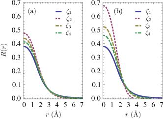
Figure 1: Radial component of the Si-$2p$ pseudo-atomic orbitals corresponding to the 4 $\zeta$ basis (4Z). (a) Multiple $\zeta$’s generated using a split norm of 0.15. In this case the additional basis functions are very similar to the first and second $\zeta$ and it is not advantageous to increase the basis size. (b) Multiple $\zeta$’s generated using a split norm of 0.5. In these case the additional orbitals are significantly different from the first and second $\zeta$ and we can expect that an increase of the basis size will improve the accuracy of the calculation.

For comparison we also perform standard planewaves calculations using the ABINIT packageGonze et al. (2009) and the YAMBO codeMarini et al. (2009), using the same Brillouin-zone grids and pseudopotentials. In the planewaves calculations dielectric matrices are obtained within the random-phase approximation using the Adler-Wiser formulation.Adler (1962); Wiser (1963) In all cases the calculations are found to be converged by using 92 unoccupied electronic states. We use planewaves cutoffs of 20 Ry for silicon and germanium and 60 Ry for diamond for the ground-state calculations. The corresponding planewaves cutoffs for the dielectric matrices are 12 Ry, 6.9 Ry, and 6.9 Ry for diamond, silicon, and germanium, respectively.

While we carefully set all the parameters of the plane-waves calculations in order to make the comparison as accurate as possible, there remains one systematic difference in how the long-wavelength limit $\mathbf{q}\rightarrow 0$ is taken in the calculation of the dielectric constant. We obtain this limit by considering a small but finite wavevector ($q=0.01\,2\pi/a$, $a$ being the lattice parameter), while the YAMBO code calculates this limit analytically. The two treatments are in principle equivalent, but we cannot rule out that this difference might result in small differences between the results presented in the following section.

IV Results and discussion

The purpose of this section is to study the convergence of the calculated dielectric matrices with the size and type of the local orbital basis, and to perform a systematic comparison with reference planewaves calculations. We discuss our results for the dielectric matrices of diamond, silicon, and germanium. We start with silicon since this has been the benchmark semiconductor in a number of previous studies of dielectric screening and quasiparticle methods.

IV.1 Macroscopic dielectric constants

IV.1.1 Silicon

Figure 2(a) shows the calculated macroscopic dielectric constant of silicon as a function of basis size, for a split norm of 0.15. The smallest possible basis includes 4 orbitals per atoms (1 $s$ orbital and 3 $p$ orbitals) and is referred to as the single-$\zeta$ basis (SZ). The basis sets with and without polarization orbitals appear to converge to different asymptotic values. The plateau of the polarized basis set is $\epsilon_{0}=12.41$ and is reached with the TZP basis (17 orbitals per atom). This value is within 3% of our reference planewaves result $\epsilon_{0}=12.85$. Interestingly the minimal polarized basis (SZP, 9 orbitals per atom) yields values which are within 10% of the reference planewaves result.

Figure 2(b) shows the effect of the split norm on the convergence of the macroscopic dielectric constant as a function of basis size. We observe that by increasing the split norm the calculated dielectric constant converges to the planewaves value more rapidly. We assign this trend to the fact that a larger split norm leads to a wider range of localization radii spanned by the additional basis functions, and hence improves the completeness of the basis set.

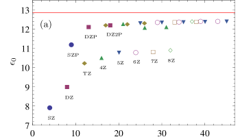
Figure 2: (a): Calculated macroscopic dielectric constant of silicon as a function of basis size, given in terms of orbitals per atom. The reference planewaves calculation is indicated by the horizontal red line. The datapoints cluster around two distinct curves: the upper curve corresponds to polarized basis sets, the lower curve to unpolarized basis sets. The number of $\zeta$ functions included is indicated by the labels SZ, DZ, TZ etc. The number of polarization orbitals for a given number of $\zeta$’s increases towards the right-hand side, as indicated for the case of the DZ basis. The energy shift is 10 meV and the split norm is 0.15. (b): Calculated macroscopic dielectric constant of silicon as a function of basis size, for two different values of the split norm.

IV.1.2 Diamond

Figure 3(a) shows the calculated macroscopic dielectric constant of diamond for a split norm of 0.15. The trend is similar to the case of silicon discussed in Sec. IV.1.1. Also in this case basis sets without polarization orbitals lead to a slower convergence rate as a function of basis size, and converge to a value significantly smaller than the reference planewaves result. The converged value for the polarized basis set is $\epsilon_{0}=5.49$ for the 4Z4P basis, which includes 36 orbitals per atom. This value agrees very well with corresponding planewaves result $\epsilon_{0}=5.47$. As in the case of silicon a reasonably converged value ($\epsilon_{0}=5.41$, 1% smaller than the planewaves result) is already obtained using the TZP basis.

Figure 3(b) shows the effect of the split norm on the convergence of the macroscopic dielectric constant as a function of basis size. In this case the trend is less clear than in Fig. 2(b), however the same general conclusions apply: by increasing the split norm the dielectric constant converges more rapidly and a plateau can be identified.

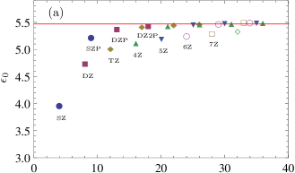
Figure 3: (a): Calculated macroscopic dielectric constant of diamond as a function of basis size, given in terms of orbitals per atom. The reference planewaves calculation is indicated by the horizontal red line. The datapoints cluster around two distinct curves: the upper curve corresponds to polarized basis sets, the lower curve to unpolarized basis sets. The number of $\zeta$ functions included is indicated by the labels SZ, DZ, TZ etc. The number of polarization orbitals for a given number of $\zeta$’s increases towards the right-hand side, as indicated for the case of the DZ basis. The energy shift is 10 meV and the split norm is 0.15. (b): Calculated macroscopic dielectric constant of diamond as a function of basis size, for two different values of the split norm.

IV.1.3 Germanium

Figure 4(a) shows the calculated macroscopic dielectric constant of germanium (split norm 0.15). Also in this case the basis sets with and without polarization orbitals appear to converge to different asymptotic values. Similarly to the case of silicon and diamond the polarized basis sets converge to a higher dielectric constant, $\epsilon_{0}=18.57$. This value is 3% larger than the reference planewave result of $\epsilon_{0}=17.94$. Also in this case we observe that the TZP basis yields a dielectric constant close to the fully converged value ($\epsilon_{0}=18.27$).

Figure 4(b) shows the effect of the split norm on the convergence of the macroscopic dielectric constant as a function of basis size. As in the other two cases, by increasing the split norm the calculated dielectric constant converges more rapidly to its asymptotic value.

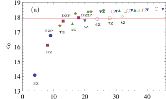
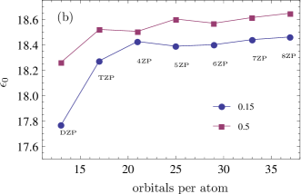
Figure 4: (a): Calculated macroscopic dielectric constant of germanium as a function of basis size, given in terms of orbitals per atom. The reference planewaves calculation is indicated by the horizontal red line. The datapoints cluster around two distinct curves: the upper curve corresponds to polarized basis sets, the lower curve to unpolarized basis sets. The number of $\zeta$ functions included is indicated by the labels SZ, DZ, TZ etc. The number of polarization orbitals for a given number of $\zeta$’s increases towards the right-hand side, as indicated for the case of the DZ basis. The energy shift is 10 meV and the split norm is 0.15. (b): Calculated macroscopic dielectric constant of germanium as a function of basis size, for two different values of the split norm.

IV.2 Frequency- and wavevector-dependent dielectric functions

Figure 5 shows the frequency-dependent dielectric function of silicon $\epsilon(\omega)$ for the minimal SZ basis set, the TZP basis set, and the reference planewaves calculation. The SZ basis performs very poorly, the spectral weight being incorrectly transferred from the main absorption peak to higher energy. This is consistent with the small value of the macroscopic dielectric constant obtained with the SZ basis in Fig. 2.

The TZP basis yields results in reasonable agreement with our reference planewaves result. The location of the main peaks and shoulders are correctly reproduced. We note, however, some transfer of spectral weight from the main peak at $\sim$4 eV to the shoulder at $\sim$3 eV, and a blueshift of the high-energy peaks.

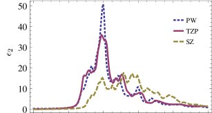
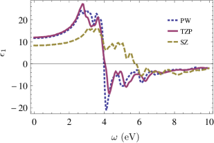
Figure 5: Calculated dielectric function of silicon: calculations using the SZ basis (dashed line), the TZP basis (solid line), and the reference planewaves result (dotted line). A Gaussian smearing of width 0.1 eV is used.

Figures 6 and 7 show the frequency-dependent dielectric functions of diamond and germanium, respectively. Also in these cases we compare the performance of the SZ basis and the TZP basis with the reference planewaves calculation. Conclusions similar to the case of silicon can be drawn: the SZ basis misses the main peak and yields a blueshift of the other peaks, while the TZP basis is in better agreement with the reference planewaves calculation.

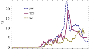
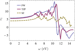
Figure 6: Calculated dielectric function of diamond: calculations using the SZ basis (dashed line), the TZP basis (solid line), and the reference planewaves result (dotted line). A Gaussian smearing of width 0.1 eV is used.

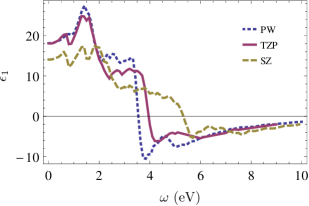
Figure 7: Calculated dielectric function of germanium: calculations using the SZ basis (dashed line), the TZP basis (solid line), and the reference planewaves result (dotted line). A Gaussian smearing of width 0.1 eV is used.

Figure 8 shows the wavevector dependence of the dielectric function $\epsilon(\mathbf{q},\omega=0)$ for silicon, diamond, and germanium, comparing the performance of the SZ and the TZP basis sets. In all cases the wavevector dependence shows the correct behavior,Walter and Cohen (1970) although the SZ basis yields a smaller dielectric function across the full range of wavevectors.

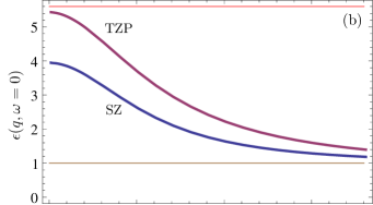
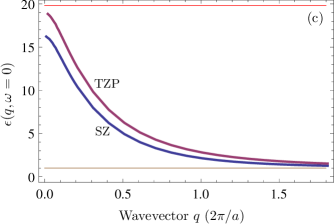
Figure 8: Wavevector dependence of the dielectric function of (a) silicon, (b) diamond, and (c) germanium. We compare the performance of the SZ and TZP basis sets. The upper horizontal line in each panel represents the static planewaves value $\epsilon_{0}$ and the lower horizontal line indicates the vacuum dielectric constant $\epsilon_{\rm vac}=1$.

V Conclusions

We reported a systematic study of the performance of numerical pseudo-atomic orbital basis sets of the SIESTA code in the calculation of dielectric matrices in extended systems using the self-consistent Sternheimer approach of Refs. Giustino et al., 2010; Hübener et al., 2012. In order to cover a range of systems from more insulating to more metallic character we presented results for the three semiconductors diamond, silicon, and germanium.

Dielectric matrices, converged within the multi-$\zeta$ and polarization scheme, fall within 3% of reference planewaves calculations, demonstrating that this method is promising. We observed that the TZP basis already yields results very close to fully converged values. This information may prove useful for practical calculations of electronic excitations using pseudo-atomic orbital basis sets as in the SIESTA code. In particular the TZP basis yields the correct spectral features in the long-wavelength frequency-dependent dielectric function.

We observed a consistent performance of the TZP basis across the three systems considered, regardless of their more insulating (diamond) or metallic (germanium) character. This may result from the different localization radii which already account for the varying degree of localization of the density matrix in each material.

We also noted that polarization orbitals are critical for achieving good agreement with reference planewaves calculations. This is somewhat expected since polarization orbitals precisely describe the response to external fields.

We have investigated how the choice of the split norm influences the convergence of the results. The increase of the split norm leads to multiple-$\zeta$ orbitals with a wider distribution of localization radii and effectively improves the completeness of the basis.

We point out that the localization radii of the basis sets discussed here are rather large and therefore are not optimal for practical calculations. Our choice was motivated by the need to systematically explore basis sets with many $\zeta$’s. We expect that similar conclusions will be obtained by augmenting the basis using diffuse numerical orbitals with similar localization radii as those considered here.Ciofini and Adamo (2007); García-Gil et al. (2009) The study of the performance of diffuse orbitals deserves further investigation.

By providing a systematic assessment of the performance of pseudo-atomic orbital basis sets including multiple-$\zeta$’s and polarization, the present work sets the ground for future studies of dielectric screening and electronic excitations in extended systems using local orbitals.

Acknowledgments

The authors would like to thank E. Artacho for fruitful discussions. This work is funded by the European Research Council under the European Community’s Seventh Framework Programme, Grant No. 239578, and Spanish MICINN Grant FIS2009-12721-C04-01.

Appendix A Bloch phase factors in the variation of the density matrix for periodic systems

The evaluation of the variation $\Delta n_{[\mathbf{q},\mathbf{r},\omega]}$ of the density matrix using Eq. (27) requires the introduction of the Bloch phase factors ${\rm exp}(i\mathbf{k}\cdot\mathbf{R})$, ${\rm exp}(i\mathbf{q}\cdot\mathbf{R})$, and ${\rm exp}(i\mathbf{q}\cdot\mathbf{r})$ at various stages. We proceed as follows.

First we merge into a single index $I$ the basis index $i$ and the unit cell vector $\mathbf{R}_{I}$ of the cell for each orbital $\phi_{i}(\mathbf{r}^{\prime}-\mathbf{R}_{I})$: $I=(i,\mathbf{R}_{I})$ and $\phi_{I}(\mathbf{r}^{\prime})=\phi_{i}(\mathbf{r}^{\prime}-\mathbf{R}_{I})$. Using this notation we rewrite Eq. (27) as follows:

$$\Delta n_{[\mathbf{q},\mathbf{r},\omega]}(\mathbf{r}^{\prime})=\frac{2}{N_{\mathbf{k}}}\sum_{v\mathbf{k}\sigma=\pm}\sum_{IJ}c^{*}_{vi\mathbf{k}}\Delta c^{\sigma}_{vj\mathbf{k}[\mathbf{q},\mathbf{r},\omega]}$$

$$\times e^{-i\mathbf{k}\cdot(\mathbf{R}_{I}-\mathbf{R}_{J})}e^{i\mathbf{q}\cdot\mathbf{R}_{J}}e^{-i\mathbf{q}\cdot\mathbf{r}^{\prime}}\phi_{I}(\mathbf{r}^{\prime})\phi_{J}(\mathbf{r}^{\prime}),$$ (28)

where $i$ in $c^{*}_{vi\mathbf{k}}$ is still the orbital component of the composite indices $I=(i,\mathbf{R}_{I})$, and similarly for $j$. In order to evaluate Eq. (28) we first calculate the matrix

$$\Delta n^{(1)}_{ij\mathbf{k}[\mathbf{q},\mathbf{r},\omega]}=2\sum_{v\sigma=\pm}c^{*}_{vi\mathbf{k}}\Delta c^{\sigma}_{vj\mathbf{k}[\mathbf{q},\mathbf{r},\omega]}.$$ (29)

Second, we perform the sum over the wavevectors $\mathbf{k}$ and introduce the phase factors ${\rm exp}[i\mathbf{k}\cdot(\mathbf{R}_{I}-\mathbf{R}_{J})]$:

$$\Delta n^{(2)}_{IJ[\mathbf{q},\mathbf{r},\omega]}=\frac{1}{N_{\mathbf{k}}}\sum_{\mathbf{k}}\Delta n^{(1)}_{ij\mathbf{k}[\mathbf{q},\mathbf{r},\omega]}e^{-i\mathbf{k}\cdot(\mathbf{R}_{I}-\mathbf{R}_{J})}.$$ (30)

Third, we include the phase factor ${\rm exp}(i\mathbf{q}\cdot\mathbf{R}_{J})$:

$$\Delta n^{(3)}_{[\mathbf{q},\mathbf{r},\omega]}(\mathbf{r}^{\prime})=\sum_{IJ}\Delta n^{(2)}_{IJ[\mathbf{q},\mathbf{r},\omega]}e^{i\mathbf{q}\cdot\mathbf{R}_{J}}\phi_{I}(\mathbf{r}^{\prime})\phi_{J}(\mathbf{r}^{\prime}),$$ (31)

and finally we introduce the factor ${\rm exp}(-i\mathbf{q}\cdot\mathbf{r})$:

$$\Delta n_{[\mathbf{q},\mathbf{r},\omega]}(\mathbf{r}^{\prime})=e^{-i\mathbf{q}\cdot\mathbf{r}}\Delta n^{(3)}_{[\mathbf{q},\mathbf{r},\omega]}(\mathbf{r}^{\prime}).$$ (32)

This final phase factor is added only after the real space density response has been evaluated on the grid.

The reason for proceeding as described here becomes evident if we make the observation that we only need to calculate the density variation inside the fundamental unit cell. This implies that we only need to work with basis orbitals belonging to the fundamental unit cell or which are nonvanishing in this cell. As a consequence we can calculate Eq. (30) only for those $I,J$ which lead to finite overlap with the fundamental cell. Furthermore, it is convenient to calculate $\Delta n^{(2)}_{IJ[\mathbf{q},\mathbf{r},\omega]}$ only for the index $I$ belonging to the fundamental unit cell [i.e. $I=(i,0)$] and the index $J$ over the orbitals with finite overlap with this cell: $J=(j^{\prime},\mathbf{R}_{J})$. This allows us to rewrite Eq. (30) as:

$$\Delta n^{(2)}_{ij^{\prime}[\mathbf{q},\mathbf{r},\omega]}=\frac{1}{N_{\mathbf{k}}}\sum_{\mathbf{k}}\Delta n^{(1)}_{ij\mathbf{k}[\mathbf{q},\mathbf{r},\omega]}e^{-i\mathbf{k}\cdot\mathbf{R}_{ij^{\prime}}},$$ (33)

where $\mathbf{R}_{ij^{\prime}}=\mathbf{R}_{I}-\mathbf{R}_{J}$ is the vector pointing from orbital $I$ to $J$ and $I$ is still $I=(i,0)$. The matrix $\Delta n^{(2)}_{ij^{\prime}[\mathbf{q},\mathbf{r},\omega]}$ in Eq. (33) has the first dimension equal to the number of orbitals in the unit cell, and the second dimension equal to the number of orbitals that are non-zero in the fundamental unit cell. This is a sparse matrix and it is stored using the sparse matrix representation of SIESTA.

The reason for evaluating Eqs. (31) and (32) separately is that the phase factor ${\rm exp}(i\mathbf{q}\cdot\mathbf{R}_{J})$ cannot be added in the same way as the $\mathbf{k}$-dependent factor into Eq. (33), since it depends on the absolute position of the cell $\mathbf{R}_{J}$ and not on the relative position of the orbitals $\mathbf{R}_{J}-\mathbf{R}_{I}$. Using this alternative notation we can rewrite Eq. (31) as:

$$\Delta n^{(3)}_{[\mathbf{q},\mathbf{r},\omega]}(\mathbf{r}^{\prime})=\sum_{i^{\prime}j^{\prime}}\Delta n^{(2)}_{ij^{\prime}[\mathbf{q},\mathbf{r},\omega]}e^{i\mathbf{q}\cdot\mathbf{R}_{j^{\prime}}}\phi_{i^{\prime}}(\mathbf{r}^{\prime})\phi_{j^{\prime}}(\mathbf{r}^{\prime}),$$ (34)

where $i^{\prime},j^{\prime}$ refer to orbitals which are non-zero in the unit cell, and $i$ is the replica of $i^{\prime}$ belonging to the fundamental unit cell.

Our procedure allows us to use the the sparse matrix $\Delta n^{(2)}_{ij^{\prime}[\mathbf{q},\mathbf{r},\omega]}$ as the working quantity for the self-consistent cycle (i.e. for charge-density mixing and convergence tests). The scheme outlined here uses the sparse matrix representation built in SIESTA and requires only small changes to existing subroutines that manage the evaluation on the real space grid. It can therefore easily make use of subroutines that manage the density matrix during the scf procedure, such as density-mixing. Furthermore, these steps ensure that the computational overhead of our procedure is minimal.

References

- Soler et al. (2002) J. M. Soler, E. Artacho, J. D. Gale, A. García, J. Junquera, P. Ordejón, and D. Sánchez-Portal, J. Phys. Condens. Matter 14, 2745 (2002).
- Skylaris et al. (2005) C.-K. Skylaris, P. D. Haynes, A. A. Mostofi, and M. C. Payne, J. Chem. Phys. 122, 084119 (2005).
- Bowler and Miyazaki (2010) D. R. Bowler and T. Miyazaki, J. Phys. Condens. Matter 22, 074207 (2010).
- Kohn (1996) W. Kohn, Phys. Rev. Lett. 76, 3168 (1996).
- Ordejón et al. (1993) P. Ordejón, D. A. Drabold, M. P. Grumbach, and R. M. Martin, Phys. Rev. B 48, 14646 (1993).
- Mauri et al. (1993) F. Mauri, G. Galli, and R. Car, Phys. Rev. B 47, 9973 (1993).
- Ordejón et al. (1996) P. Ordejón, E. Artacho, and J. M. Soler, Phys. Rev. B 53, R10441 (1996).
- Goedecker (1999) S. Goedecker, Rev. Mod. Phys. 71, 1085 (1999).
- Hedin (1965) L. Hedin, Phys. Rev. 139, A796 (1965).
- Hybertsen and Louie (1986) M. S. Hybertsen and S. G. Louie, Phys. Rev. B 34, 5390 (1986).
- Ihm et al. (1979) J. Ihm, A. Zunger, and M. L. Cohen, J. Phys. C: Solid State Phys. 12, 4409 (1979).
- Chelikowsky et al. (1994) J. R. Chelikowsky, N. Troullier, and Y. Saad, Phys. Rev. Lett. 72, 1240 (1994).
- Bruneval and Gonze (2008) F. Bruneval and X. Gonze, Phys. Rev. B 78, 085125 (2008).
- Berger et al. (2010) J. A. Berger, L. Reining, and F. Sottile, Phys. Rev. B 82, 041103 (2010).
- Wilson et al. (2008) H. F. Wilson, F. Gygi, and G. Galli, Phys. Rev. B 78, 113303 (2008).
- Wilson et al. (2009) H. F. Wilson, D. Lu, F. Gygi, and G. Galli, Phys. Rev. B 79, 245106 (2009).
- Giustino et al. (2010) F. Giustino, M. L. Cohen, and S. G. Louie, Phys. Rev. B 81, 115105 (2010).
- Umari et al. (2010) P. Umari, G. Stenuit, and S. Baroni, Phys. Rev. B 81, 115104 (2010).
- Hübener et al. (2012) H. Hübener, M. A. Pérez-Osorio, P. Ordejón, and F. Giustino, (2012), arXiv:1202.XXXX.
- Baroni et al. (1987) S. Baroni, P. Giannozzi, and A. Testa, Phys. Rev. Lett. 58, 1861 (1987).
- Baroni et al. (2001) S. Baroni, S. de Gironcoli, A. Dal Corso, and P. Giannozzi, Rev. Mod. Phys. 73, 515 (2001).
- Aryasetiawan and Gunnarsson (1994) F. Aryasetiawan and O. Gunnarsson, Phys. Rev. B 49, 16214 (1994).
- Rohlfing et al. (1995) M. Rohlfing, P. Krüger, and J. Pollmann, Phys. Rev. B 52, 1905 (1995).
- Blase and Ordejón (2004) X. Blase and P. Ordejón, Phys. Rev. B 69, 085111 (2004).
- Koval et al. (2010) P. Koval, D. Foerster, and O. Coulaud, Phys. Status Solidi B 247, 1841–1848 (2010).
- Foerster et al. (2011) D. Foerster, P. Koval, and D. Sanchez-Portal, J. Chem. Phys. 135, 074105 (2011).
- Blase et al. (2011) X. Blase, C. Attaccalite, and V. Olevano, Phys. Rev. B 83, 115103 (2011).
- Troullier and Martins (1991) N. Troullier and J. L. Martins, Phys. Rev. B 43, 1993 (1991).
- Artacho et al. (1999) E. Artacho, D. Sánchez-Portal, P. Ordejón, A. García, and J. M. Soler, Phys. Status Solidi B 215, 809 (1999).
- Sánchez-Portal et al. (1996) D. Sánchez-Portal, E. Artacho, and J. M. Soler, J. Phys. Condens. Matter 8, 3859 (1996).
- Junquera et al. (2001) J. Junquera, O. Paz, D. Sánchez-Portal, and E. Artacho, Phys. Rev. B 64, 235111 (2001).
- Ceperley and Alder (1980) D. M. Ceperley and B. J. Alder, Phys. Rev. Lett. 45, 566 (1980).
- Perdew and Zunger (1981) J. P. Perdew and A. Zunger, Phys. Rev. B 23, 5048 (1981).
- Hybertsen and Louie (1987) M. S. Hybertsen and S. G. Louie, Phys. Rev. B 35, 5585 (1987).
- Gonze et al. (2009) X. Gonze, B. Amadon, P.-M. Anglade, J.-M. Beuken, F. Bottin, P. Boulanger, F. Bruneval, D. Caliste, R. Caracas, M. Côté, T. Deutsch, L. Genovese, P. Ghosez, M. Giantomassi, S. Goedecker, D. Hamann, P. Hermet, F. Jollet, G. Jomard, S. Leroux, M. Mancini, S. Mazevet, M. Oliveira, G. Onida, Y. Pouillon, T. Rangel, G.-M. Rignanese, D. Sangalli, R. Shaltaf, M. Torrent, M. Verstraete, G. Zerah, and J. Zwanziger, Comput. Phys. Commun. 180, 2582 (2009).
- Marini et al. (2009) A. Marini, C. Hogan, M. Grüning, and D. Varsano, Comput. Phys. Commun. 180, 1392 (2009).
- Note (1) We note that there is a small difference between SIESTA and ABINIT in how the local part of the pseudopotential is constructed.
- Adler (1962) S. L. Adler, Phys. Rev. 126, 413 (1962).
- Wiser (1963) N. Wiser, Phys. Rev. 129, 62 (1963).
- Walter and Cohen (1970) J. P. Walter and M. L. Cohen, Phys. Rev. B 2, 1821 (1970).
- Ciofini and Adamo (2007) I. Ciofini and C. Adamo, J. Phys. Chem. A 111, 5549 (2007).
- García-Gil et al. (2009) S. García-Gil, A. García, N. Lorente, and P. Ordejón, Phys. Rev. B 79, 075441 (2009).