Dielectric screening in extended systems
using the self-consistent Sternheimer equation and localized basis sets

Abstract

We develop a first-principles computational method for investigating the dielectric screening in extended systems using the self-consistent Sternheimer equation and localized non-orthogonal basis sets. Our approach does not require the explicit calculation of unoccupied electronic states, only uses two-center integrals, and has a theoretical scaling of order $O(N^{3})$. We demonstrate this method by comparing our calculations for silicon, germanium, diamond, and LiCl with reference planewaves calculations. We show that accuracy comparable to planewaves calculations can be achieved via a systematic optimization of the basis set.

Quasiparticle calculations based on the $GW$ method Hedin (1965); Hedin and Lundqvist (1969); Hybertsen and Louie (1986); Aryasetiawan and Gunnarsson (1998); Aulbur et al. (2000); Onida et al. (2002) and calculations of optical spectra using the Bethe-Salpeter equation Onida et al. (1995); Rohlfing and Louie (1998); Onida et al. (2002) have emerged as state-of-the-art first-principles computational methods for the study of electronic and optical excitations both in extended solids and in nanoscale systems. While in many cases these methods can reproduce and even predict experimental photoemission and optical data with remarkable accuracy, the associated computational complexity limits their application to relatively small systems, typically in the range of ten to a hundred atoms. The main bottleneck in these calculations is the evaluation of the irreducible polarization propagator in the random-phase approximation (RPA), which is used for constructing the screened Coulomb interaction of the $GW$ self-energy, and the electron-hole interaction kernel in the Bethe-Salpeter equation. The calculation of this propagator is performed using an expansion over unoccupied Kohn-Sham states Hybertsen and Louie (1986); Rohlfing et al. (1993, 1995); Aryasetiawan and Gunnarsson (1998); Aulbur et al. (2000); Onida et al. (2002); Blase et al. (2011), and has a theoretical scaling of $O(N^{4})$, $N$ being the number of atoms in the system Giustino et al. (2010) . In addition the polarization propagator is commonly calculated by expanding the Kohn-Sham states using planewaves basis sets Ihm et al. (1979). While planewaves have several obvious advantages, large systems can become intractable due to the very large basis size. These observations clearly point to the need for new methods to study the dielectric screening in complex systems which (i) do not require the explicit calculation of unoccupied electronic states, (ii) use small basis sets, and (iii) exhibit a more favorable scaling with system size.

Several methods have been proposed in order to avoid the explicit calculation of unoccupied electronic states in the study of electronic excitations Levine and Allan (1989, 1991); Reining et al. (1997); Andrade et al. (2007); Wilson et al. (2008); Bruneval and Gonze (2008); Wilson et al. (2009); Rocca et al. (2010); Giustino et al. (2010); Umari et al. (2010); Berger et al. (2010). Some of these methods rely on the Sternheimer equation Levine and Allan (1989, 1991); Reining et al. (1997); Andrade et al. (2007); Giustino et al. (2010), which is routinely used in density-functional perturbation theory Baroni et al. (2001), and closely related to the coupled-perturbed Hartree-Fock method found in the quantum chemistry literature McWeeny (1962); Gerratt (1968); Liang et al. (2005). In particular, in Ref. Giustino et al. (2010) the Sternheimer method is used self-consistently in order to calculate the full frequency-dependent inverse dielectric function in extended systems, and an empirical pseudopotential implementation is described as a proof-of-concept.

In order to reduce the computational complexity of Sternheimer-type approaches it appears advantageous to adapt these methods to the case of localized basis sets. Indeed, electronic structure codes based on localized representations are successfully employed to study very large systems, up to several thousands of atoms Soler et al. (2002); Skylaris et al. (2005); Bowler and Miyazaki (2010). The key advantage of these basis sets is that they exploit the electron localization in the insulating state Kohn (1996) in order to obtain a sparse representation of the ground-state density matrix. However, since these basis sets are optimized for providing an accurate description of the occupied Kohn-Sham manifold, it is not clear a priori what their performance would be in the case of excited state calculations.

In this work we demonstrate a first-principles pseudopotential scheme for calculating the inverse dielectric matrix in extended systems using non-orthogonal localized basis sets. Our scheme includes both local-field effects and the frequency-dependence of the inverse dielectric matrix, and does not require the explicit calculation of unoccupied Kohn-Sham states. This is achieved by adapting the self-consistent Sternheimer method of Ref. Giustino et al. (2010) to the case of a basis set of localized pseudo-atomic orbitals as implemented in the SIESTA code Sánchez-Portal et al. (1996); Artacho et al. (1999); Soler et al. (2002). Here we illustrate the formalism and report calculations of the inverse dielectric matrix for prototypical semiconductors and insulators. We perform a systematic comparison with reference planewaves calculations, and we investigate the convergence of our results with the size of the local orbital basis set. A detailed report with extensive benchmarks and implementation details is provided elsewhere Hübener et al. (2012).

We calculate the inverse dielectric matrix in the random-phase approximation following Ref. Giustino et al. (2010). The frequency-dependent variation of the density matrix $\Delta n(\mathbf{r},\mathbf{r}^{\prime},\omega)$ corresponding to the non-local bare Coulomb potential $v(\mathbf{r},\mathbf{r}^{\prime})$ is given by:

$$\Delta n(\mathbf{r},\mathbf{r}^{\prime},\omega)=2\!\sum_{v,\sigma=\pm}\psi^{*}_{v}(\mathbf{r}^{\prime})\Delta\psi_{v}(\mathbf{r},\mathbf{r}^{\prime},\sigma\omega),$$ (1)

where $\psi_{v}$ is an occupied Kohn-Sham state of energy $\epsilon_{v}$ and spin-unpolarized systems are considered for simplicity. The variations $\Delta\psi_{v}(\mathbf{r},\mathbf{r}^{\prime},\pm\omega)$ of the single-particle states are solutions of the Sternheimer equations:

$$(\hat{H}-\epsilon_{v}\pm\omega)\Delta\psi_{v}(\mathbf{r},\mathbf{r}^{\prime},\pm\omega)=-(1-\hat{P}_{v})W(\mathbf{r},\mathbf{r}^{\prime},\omega)\psi_{v}(\mathbf{r}^{\prime}),$$ (2)

where Kohn-Sham Hamiltonian $\hat{H}$ and the projector $\hat{P}_{v}$ on the occupied manifold act on the variable $\mathbf{r}^{\prime}$, and $W(\mathbf{r},\mathbf{r}^{\prime},\omega)$ is the RPA frequency-dependent screened Coulomb interaction. In order to obtain the screened Coulomb interaction we use the change $\Delta V_{H}$ of the Hartree potential resulting from the variation of the density matrix:

$$\Delta V_{H}(\mathbf{r},\mathbf{r}^{\prime},\omega) = \int d\mathbf{r}^{\prime\prime}\Delta n(\mathbf{r},\mathbf{r}^{\prime\prime},\omega)v(\mathbf{r}^{\prime\prime},\mathbf{r}^{\prime}),$$ (3)

$$W(\mathbf{r},\mathbf{r}^{\prime},\omega) = v(\mathbf{r},\mathbf{r}^{\prime})+\Delta V_{H}(\mathbf{r},\mathbf{r}^{\prime},\omega).$$ (4)

Equations (1)-(4) need to be solved self-consistently. In the following we use this formalism in order to directly calculate the inverse dielectric matrix $\epsilon^{-1}(\mathbf{r},\mathbf{r}^{\prime},\omega)$. This is done by replacing $W$ in Eq. (2) by $\epsilon^{-1}$, and by using the following relation instead of Eq. (4):

$$\epsilon^{-1}(\mathbf{r},\mathbf{r}^{\prime},\omega)=\delta(\mathbf{r},\mathbf{r}^{\prime})+\Delta V_{H}(\mathbf{r},\mathbf{r}^{\prime},\omega).$$ (5)

In this case the self-consistent calculation is started by initializing the inverse dielectric matrix to the Dirac delta $\delta(\mathbf{r},\mathbf{r}^{\prime})$. A derivation of the connection with the sum-over-states approach and details on this formalism can be found in Refs. Giustino et al. (2010); Hübener et al. (2012) respectively.

We now move to a localized basis representation. We first make the choice of treating the variables $\mathbf{r}$ and $\omega$ in the Sternheimer equation Eq. (2) as parameters. The variable $\mathbf{r}$ will be represented on a real-space grid. Then we expand the quantities dependent on $\mathbf{r}^{\prime}$ in the basis of local orbitals $\phi_{i}(\mathbf{r}^{\prime})$:

$$\psi_{v}(\mathbf{r}^{\prime}) = \sum_{i}c_{vi}\phi_{i}(\mathbf{r}^{\prime})$$ (6)

$$\Delta\psi^{\pm}_{v[\mathbf{r},\omega]}(\mathbf{r}^{\prime}) = \sum_{i}\Delta c^{\pm}_{vi[\mathbf{r},\omega]}\phi_{i}(\mathbf{r}^{\prime}).$$ (7)

By replacing Eqs. (6),(7) in Eq. (2) and projecting both sides onto $\phi_{j}(\mathbf{r}^{\prime})$ we obtain the Sternheimer equation in matrix representation:

$$\left[\mathbf{H}-(\epsilon_{v}\pm\omega)\mathbf{S}\right]\Delta\mathbf{c}^{\pm}_{v[\mathbf{r},\omega]}=-\left[\mathbf{1}-\mathbf{S}\mbox{\boldmath$\rho$}^{T}\right]\Delta\mathbf{V}_{[\mathbf{r},\omega]}\mathbf{c}_{v}.$$ (8)

Here $\mathbf{H}$, $\mathbf{S}$ and $\rho$ are the Kohn-Sham Hamiltonian, the overlap, and the density matrices, respectively. The matrix elements of $\Delta\mathbf{V}_{[\mathbf{r},\omega]}$ in Eq. (8) are defined as:

$$\Delta V_{ij[\mathbf{r},\omega]}=\int d\mathbf{r}^{\prime}\phi^{*}_{i}(\mathbf{r}^{\prime})\Delta V_{[\mathbf{r},\omega]}(\mathbf{r}^{\prime})\phi_{j}(\mathbf{r}^{\prime}).$$ (9)

The solution of Eq. (8) yields the coefficients $\Delta\mathbf{c}^{\pm}_{v[\mathbf{r},\omega]}$ which are used to construct the variation of the density matrix from Eq. (1):

$$\Delta n_{ij[\mathbf{r},\omega]}=2\sum_{v,\sigma=\pm}c^{*}_{vi}\Delta c^{\sigma}_{vj[\mathbf{r},\omega]}.$$ (10)

At this point it is possible to explicitly calculate $\Delta n(\mathbf{r},\mathbf{r}^{\prime},\omega)$ on a real-space grid, and then perform the integral in Eq. (3) on the same grid. Equation (4) is also evaluated on the real space grid, and the resulting potential is projected on the local orbital basis using Eq. (9). This procedure is repeated until self-consistency is achieved, and is carried out independently for each value of the parameters $\mathbf{r}$ and $\omega$.

For the purpose of comparison with standard planewaves calculations it is convenient to specialize this formalism to the case of crystalline solids. We proceed as follows: we incorporate the Bloch phase factors in the basis orbitals $\phi_{i\mathbf{k}}(\mathbf{r}^{\prime})$

$$\phi_{i\mathbf{k}}(\mathbf{r}^{\prime})=\sum_{\mathbf{R}}e^{-i\mathbf{k}\cdot(\mathbf{r}-\mathbf{R})}\phi_{i}(\mathbf{r}^{\prime}-\mathbf{R}),$$ (11)

where $\mathbf{k}$ is a wavevector in the Brillouin zone, and $\mathbf{R}$ is a lattice vector. The orbitals $\phi_{i}$ in Eq. (11) are the same as in Eq. (6), except that now the index $i$ runs over the orbitals spanning one unit cell only. Equation (11) defines a basis of periodic functions and is used to expand the cell-periodic part $u_{v\mathbf{k}}$ of the Bloch states $\psi_{v\mathbf{k}}(\mathbf{r}^{\prime})=e^{i\mathbf{k}\cdot\mathbf{r}^{\prime}}u_{v\mathbf{k}}(\mathbf{r}^{\prime})$. By using a similar expansion for the variations of the wavefunctions in Eq. (7), and by projecting both sides of Eq. (2) on the basis orbitals, we obtain the Sternheimer equation for periodic systems:

$$\begin{split}&\left[\mathbf{H}_{\mathbf{k}+\mathbf{q}}-(\epsilon_{v\mathbf{k}}\pm\omega)\mathbf{S}_{\mathbf{k}+\mathbf{q}}\right]\Delta\mathbf{c}^{\pm}_{v\mathbf{k}[\mathbf{q},\mathbf{r},\omega]}=\\ &\qquad\qquad\;-\left[\mathbf{1}-\mathbf{S}_{\mathbf{k}+\mathbf{q}}\mathbf{\mbox{\boldmath$\rho$}}^{T}_{\mathbf{k}+\mathbf{q}}\right]\Delta\mathbf{V}_{\mathbf{k}[\mathbf{q},\mathbf{r},\omega]}\mathbf{c}_{v\mathbf{k}},\end{split}$$ (12)

which is analogous to Eq. (8). In this case the Hamiltonian, overlap, and density matrices, as well as the coefficient vectors, are all resolved in momentum space. A detailed derivation of these equations is provided in Ref. Hübener et al. (2012).

In the present formalism the dependence on the real-space variable $\mathbf{r}^{\prime}$ is represented on the local orbital basis, while the dependence on $\mathbf{r}$ is represented on a real-space grid. This choice carries the following advantages: (i) we do not use a product-basis expansion for non-local quantities, therefore we avoid issues related to the representability of the screened Coulomb interaction in localized basis sets. (ii) We only have two-center integrals in our formulation, therefore we do not need the three and four-center integrals arising in product basis expansions Rohlfing et al. (1995); Blase and Ordejón (2004); Koval et al. (2010); Foerster et al. (2011); Blase et al. (2011). (iii) The self-consistent calculation of the inverse dielectric matrix avoids from the outset the issues associated with the inversion of response functions represented in local orbital basis sets Gidopoulos and Lathiotakis (2011). (iv) Since Eq. (8) can be solved using sparse linear algebra and needs to be performed for every occupied state and every $\mathbf{r}$ on the real-space grid, this method has a theoretical scaling of $O(N^{3})$.

The key approximation in our formulation is the expansion of the variation $\Delta\psi^{\pm}_{v[\mathbf{r},\omega]}$ of the single-particle states in the basis of local orbital [cf. Eq.(7)]. In fact local orbital basis sets are typically optimized to accurately describe the occupied states manifold, while the variation of the density matrix arises from the components of $\Delta\psi^{\pm}_{v[\mathbf{r},\omega]}$ in the manifold of unoccupied states Baroni et al. (2001). This clearly points to the need of carefully optimizing the local orbital basis sets for calculations of the dielectric screening. A systematic assessment of the performance of multiple-$\zeta$ polarized pseudo-atomic orbital basis sets is provided in Ref. Hübener et al. (2012).

Our implementation is based on the SIESTA code, and uses a basis of strictly localized numerical pseudo-atomic orbitals Sánchez-Portal et al. (1996); Artacho et al. (1999); Soler et al. (2002). In the following we discuss benchmark results for silicon, diamond, germanium and LiCl. Calculations are performed within the local-density approximation (LDA) to density-functional theory Ceperley and Alder (1980); Perdew and Zunger (1981), and with norm-conserving pseudopotentials Troullier and Martins (1991). The inverse dielectric matrices are calculated by sampling the Brillouin zone using a shifted 10$\times$10$\times$10 grid for diamond, silicon and LiCl, and a shifted 12$\times$12$\times$12 grid for germanium. We use the lattice parameters 5.43 Å, 3.56 Å, 5.65 Å, and 5.13 Å for silicon, diamond, germanium, and LiCl, respectively Hybertsen and Louie (1987). Using a standard triple-$\zeta$ polarized (TZP) basis we obtain direct band gaps of 2.55 eV (Si), 5.60 eV (diamond), 0.04 eV (Ge), 5.99 eV (LiCl), in line with standard LDA results. In order to generate basis sets for silicon with a large number of $\zeta$’s we use an energy-shift parameter Artacho et al. (1999) of 10 meV. This shift leads to localization radius of 9.3 Å for silicon which is slightly larger than those adopted in standard ground-state calculations using SIESTA. We compare our results with planewaves calculations performed using ABINIT Gonze et al. (2009) and YAMBO Marini et al. (2009) software packages, with same the pseudopotentials and Brillouin-zone sampling for consistency . Planewaves calculations are carried out using kinetic energy cutoffs of 20 Ry for Si and Ge, and of 60 Ry for diamond and LiCl. The RPA dielectric matrices are calculated using 92 conduction bands and kinetic energy cutoffs of 6.9 Ry for silicon, germanium and LiCl, and of 12 Ry for diamond.

Figure 1 shows the calculated static macroscopic dielectric constant of silicon as a function of basis set size. The size of the basis is increased by including additional $\zeta$’s using the split-norm procedure, as well as polarization orbitals Artacho et al. (1999). We find that the single-$\zeta$ polarized (SZP) basis already gives results which are within 10% of the reference planewaves calculation. This suggests that a suitably optimized basis with a few orbitals should be able to yield converged results. We also observe a monotonic convergence with the number of basis orbitals, and a consistently superior performance of the basis sets including polarization orbitals (Fig. 1).

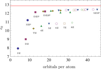
Figure 1: Calculated macroscopic dielectric constant of silicon $\epsilon_{0}=1/\epsilon^{-1}_{{\bf 0}{\bf 0}}({\bf q}\rightarrow 0,\omega=0)$ as a function of basis size, given in terms of orbitals per atom [we use ${\bf q}=2\pi/a(0.01,0,0)$, $a$ being the Si lattice constant]. The number of $\zeta$ functions included in each basis set is indicated by the labels SZ, DZ, TZ, etc. The number of polarization orbitals included in each basis set increases towards the right-hand side, as indicated for the case of the DZ basis. The reference planewaves calculation is indicated by the horizontal line.

We can rationalize the convergence of the dielectric constant with basis size shown in Fig. 1 by considering the Penn model for the dielectric constants of semiconductors Penn (1962). In this simple model the dielectric constant is related to the Penn gap $E_{\rm P}$ and to the plasma frequency $\omega_{\rm p}$ by $\epsilon_{0}=1+(\hbar\omega_{\rm p}/E_{\rm P})^{2}$. In our calculations we extract the Penn gap for each basis set considered in Fig. 1 using the main peak in the joint density of states (JDOS) Cardona and Yu (1999) . Figure 2 shows that $\epsilon_{0}-1$ is approximately a linear function of $1/E_{\rm P}^{2}$. In particular the values calculated using the unpolarized basis sets nicely fall on the line obtained using the plasma frequency of silicon $\hbar\omega_{\rm p}$ =16.6 eV. For comparison, the inset of Fig. 2 shows that the calculated dielectric constants do not correlate with the direct band gap of silicon. These observations lead us to conclude that the Penn gap, and more generally the low-energy structure of the JDOS, is a good indicator of the quality of the basis set for calculating dielectric constants. This is helpful for a quick assessment of the quality of a basis set without explicitly calculating the screening.

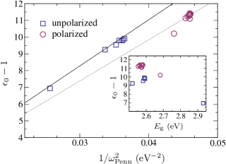
Figure 2: Macroscopic dielectric constant of silicon vs. Penn gap, plotted as $\epsilon_{0}-1$ vs. $1/E_{\rm P}^{2}$, with unpolarized (squares) and polarized (circles) basis sets. The slope of the solid line corresponds to the square of the plasma frequency of silicon, the dotted line is a guide to the eye. Inset: macroscopic dielectric constant vs. the direct band gap $E_{\rm g}$.

Table 1 shows the first few elements of the inverse dielectric matrix $\epsilon^{-1}_{{\bf G}{\bf G}^{\prime}}({\bf q}\rightarrow 0,\omega=0)$ for several local orbital basis sets. We observe that the calculated values for the first few shells compare well with the reference planewaves calculation, similarly to the head of the dielectric matrix. For higher shells, however, the relative agreement of the basis sets worsens slightly. This may indicate a systematic deficiency in the local orbital basis in case of the higher Fourier components of dielectric matrix, and clearly deserves further investigation.

$\mathbf{G}$	$\mathbf{G}^{\prime}$	SZ	TZP	CZ4P	PW
(0,0,0)	(0,0,0)	0.125	0.081	0.080	0.077
(1,1,1)	(1,1,1)	0.822	0.617	0.600	0.637
(1,1,1)	(2,0,0)	-0.037	-0.040	-0.036	-0.038
(2,0,0)	(2,0,0)	0.839	0.686	0.664	0.766
(2,2,2)	(2,2,2)	0.984	0.952	0.937	0.984
(2,2,2)	(1,1,1)	-0.009	-0.030	-0.034	-0.020
(2,2,2)	(2,0,0)	-0.003	0.003	0.005	0.002

Table 1: Fourier components of the symmetrized inverse dielectric matrix $\epsilon^{-1}_{{\bf G}{\bf G}^{\prime}}({\bf q}\rightarrow 0,\omega=0)$ of silicon, calculated using the SZ basis (4 orbitals per atom), TZP (17 orbitals per atom), the CZ4P basis (40 orbitals per atom), and a planewaves (PW) basis set. The reciprocal lattice vectors are given in units of $2\pi/a$, $a$ being the Si lattice parameter.

Figure 3 shows the frequency-dependent dielectric function of silicon calculated using our method, together with a reference planewaves calculation. We observe that, as expected, the performance of the minimal single-$\zeta$ basis is poor. In fact, spectral weight is incorrectly transferred from the main absorption peak to higher energies. On the contrary, the TZP basis (17 orbitals per atom) performs quite well, with all the main features of the planewaves spectra correctly reproduced. We still observe however some small transfer of spectral weight and a slight blueshift of the high-energy peaks.

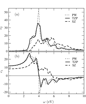
Figure 3: Macroscopic dielectric function of silicon $\epsilon(\omega)=\epsilon^{-1}_{{\bf 0}{\bf 0}}({\bf q}\rightarrow 0,\omega)$ as a function of frequency: (a) imaginary part $\epsilon_{2}(\omega)$, and (b) real part $\epsilon_{1}(\omega)$. We compare our calculations performed using the SZ basis (dashed lines) and the TZP basis (solid lines) with reference planewaves calculations (dotted lines). We use an energy broadening of 0.1 eV.

In order to demonstrate the generality of of our approach we present in Tab. 2 our calculated dielectric constants for germanium, diamond, and LiCl. The values shown in Tab. 2 are obtained by using standard SIESTA settings for the basis . Table 2 provides further support to our previous finding by showing that the TZP basis provides results which lie within 1-5% of the reference planewaves calculations. We expect further improvement upon designing basis sets specifically optimized for the Sternheimer scheme proposed in this work. In particular the use of numerical diffuse orbitals Ciofini and Adamo (2007); García-Gil et al. (2009) deserves a systematic assessment.

	SZ	TZP	PW	Expt.
Si	8.41	12.25	12.84	11.7a
Ge	15.38	18.15	17.92	15.8a
Diamond	3.94	5.43	5.47	5.5a
LiCl	1.69	2.68	2.82	2.8b

^(a) Ref. Kittel (1986).

^(b) Ref. Ashcroft and Mermin (1976).

Table 2: Dielectric constants of Si, Ge, diamond, and LiCl calculated using our Sternheimer approach, and compared to reference planewaves calculations and experimental data. We report both our results obtained using the minimal SZ basis and the TZP basis, as generated using the standard settings of SIESTA.

In conclusion, we have introduced and demonstrated a method for calculating the inverse dielectric matrix of extended systems combining localized non-orthogonal basis sets with the self-consistent Sternheimer equation. Our method does not require the calculation of unoccupied electronic states, does not require the explicit inversion of the dielectric matrix, uses only two-center integrals, and has a theoretical scaling with system size of $O(N^{3})$. Our implementation based on the pseudo-atomic orbitals of the SIESTA code shows that results with accuracy comparable to planewaves calculations can be obtained upon optimization of the localized basis set. Our formulation is completely general and there should be no difficulties in adapting our method to other local basis implementations. We believe this work represents a stepping stone towards quasiparticle $GW$ calculations for large and complex systems using localized basis sets.

The authors would like to thank E. Artacho for fruitful discussions. This work is funded by the European Research Council under the European Community’s Seventh Framework Programme, Grant No. 239578, and Spanish MICINN Grant FIS2009-12721-C04-01.

References

- Hedin (1965) L. Hedin, Phys. Rev. 139, A796 (1965).
- Hedin and Lundqvist (1969) L. Hedin and S. Lundqvist, Solid State Physics, edited by F. Seitz, D. Turnbull, and A. Ehrenreich, Vol. 23 (Academic Press, New York, 1969) p. 1.
- Hybertsen and Louie (1986) M. S. Hybertsen and S. G. Louie, Phys. Rev. B 34, 5390 (1986).
- Aryasetiawan and Gunnarsson (1998) F. Aryasetiawan and O. Gunnarsson, Rep. Prog. Phys. 61, 237 (1998).
- Aulbur et al. (2000) W. G. Aulbur, L. Jönsson, and J. W. Wilkins, Solid State Physics, edited by A. Ehrenreich and F. Spaepen, Vol. 54 (Academic, San Diego, 2000) p. 1.
- Onida et al. (2002) G. Onida, L. Reining, and A. Rubio, Rev. Mod. Phys. 74, 601 (2002).
- Onida et al. (1995) G. Onida, L. Reining, R. W. Godby, R. Del Sole, and W. Andreoni, Phys. Rev. Lett. 75, 818 (1995).
- Rohlfing and Louie (1998) M. Rohlfing and S. G. Louie, Phys. Rev. Lett. 81, 2312 (1998).
- Rohlfing et al. (1993) M. Rohlfing, P. Krüger, and J. Pollmann, Phys. Rev. B 48, 17791 (1993).
- Rohlfing et al. (1995) M. Rohlfing, P. Krüger, and J. Pollmann, Phys. Rev. B 52, 1905 (1995).
- Blase et al. (2011) X. Blase, C. Attaccalite, and V. Olevano, Phys. Rev. B 83, 115103 (2011).
- Giustino et al. (2010) F. Giustino, M. L. Cohen, and S. G. Louie, Phys. Rev. B 81, 115105 (2010).
- Note (1) By using planewaves basis sets and fast Fourier transform techniques a scaling can be obtained.
- Ihm et al. (1979) J. Ihm, A. Zunger, and M. L. Cohen, J. Phys. C: Solid State Phys. 12, 4409 (1979).
- Levine and Allan (1989) Z. H. Levine and D. C. Allan, Phys. Rev. Lett. 63, 1719 (1989).
- Levine and Allan (1991) Z. H. Levine and D. C. Allan, Phys. Rev. B 43, 4187 (1991).
- Reining et al. (1997) L. Reining, G. Onida, and R. W. Godby, Phys. Rev. B 56, R4301 (1997).
- Andrade et al. (2007) X. Andrade, S. Botti, M. A. L. Marques, and A. Rubio, J. Chem. Phys. 126, 184106 (2007).
- Wilson et al. (2008) H. F. Wilson, F. Gygi, and G. Galli, Phys. Rev. B 78, 113303 (2008).
- Bruneval and Gonze (2008) F. Bruneval and X. Gonze, Phys. Rev. B 78, 085125 (2008).
- Wilson et al. (2009) H. F. Wilson, D. Lu, F. Gygi, and G. Galli, Phys. Rev. B 79, 245106 (2009).
- Rocca et al. (2010) D. Rocca, D. Lu, and G. Galli, J. Chem. Phys. 133, 164109 (2010).
- Umari et al. (2010) P. Umari, G. Stenuit, and S. Baroni, Phys. Rev. B 81, 115104 (2010).
- Berger et al. (2010) J. A. Berger, L. Reining, and F. Sottile, Phys. Rev. B 82, 041103 (2010).
- Baroni et al. (2001) S. Baroni, S. de Gironcoli, A. Dal Corso, and P. Giannozzi, Rev. Mod. Phys. 73, 515 (2001).
- McWeeny (1962) R. McWeeny, Phys. Rev. 126, 1028 (1962).
- Gerratt (1968) J. Gerratt, J. Chem. Phys. 49, 1719 (1968).
- Liang et al. (2005) W. Liang, Y. Zhao, and M. Head-Gordon, J. Chem. Phys. 123, 194106 (2005).
- Soler et al. (2002) J. M. Soler, E. Artacho, J. D. Gale, A. García, J. Junquera, P. Ordejón, and D. Sánchez-Portal, J. Phys. Condens. Matter 14, 2745 (2002).
- Skylaris et al. (2005) C.-K. Skylaris, P. D. Haynes, A. A. Mostofi, and M. C. Payne, J. Chem. Phys. 122, 084119 (2005).
- Bowler and Miyazaki (2010) D. R. Bowler and T. Miyazaki, J. Phys. Condens. Matter 22, 074207 (2010).
- Kohn (1996) W. Kohn, Phys. Rev. Lett. 76, 3168 (1996).
- Sánchez-Portal et al. (1996) D. Sánchez-Portal, E. Artacho, and J. M. Soler, J. Phys. Condens. Matter 8, 3859 (1996).
- Artacho et al. (1999) E. Artacho, D. Sánchez-Portal, P. Ordejón, A. García, and J. M. Soler, Phys. Status Solidi B 215, 809 (1999).
- Hübener et al. (2012) H. Hübener, M. A. Pérez-Osorio, P. Ordejón, and F. Giustino, (2012), arXiv:1202.XXXX.
- Blase and Ordejón (2004) X. Blase and P. Ordejón, Phys. Rev. B 69, 085111 (2004).
- Koval et al. (2010) P. Koval, D. Foerster, and O. Coulaud, Phys. Status Solidi B 247, 1841–1848 (2010).
- Foerster et al. (2011) D. Foerster, P. Koval, and D. Sanchez-Portal, J. Chem. Phys. 135, 074105 (2011).
- Gidopoulos and Lathiotakis (2011) N. I. Gidopoulos and N. N. Lathiotakis, (2011), arXiv:1107.6007.
- Ceperley and Alder (1980) D. M. Ceperley and B. J. Alder, Phys. Rev. Lett. 45, 566 (1980).
- Perdew and Zunger (1981) J. P. Perdew and A. Zunger, Phys. Rev. B 23, 5048 (1981).
- Troullier and Martins (1991) N. Troullier and J. L. Martins, Phys. Rev. B 43, 1993 (1991).
- Hybertsen and Louie (1987) M. S. Hybertsen and S. G. Louie, Phys. Rev. B 35, 5585 (1987).
- Gonze et al. (2009) X. Gonze, B. Amadon, P.-M. Anglade, J.-M. Beuken, F. Bottin, P. Boulanger, F. Bruneval, D. Caliste, R. Caracas, M. Côté, T. Deutsch, L. Genovese, P. Ghosez, M. Giantomassi, S. Goedecker, D. Hamann, P. Hermet, F. Jollet, G. Jomard, S. Leroux, M. Mancini, S. Mazevet, M. Oliveira, G. Onida, Y. Pouillon, T. Rangel, G.-M. Rignanese, D. Sangalli, R. Shaltaf, M. Torrent, M. Verstraete, G. Zerah, and J. Zwanziger, Comput. Phys. Commun. 180, 2582 (2009).
- Marini et al. (2009) A. Marini, C. Hogan, M. Grüning, and D. Varsano, Comput. Phys. Commun. 180, 1392 (2009).
- Note (2) We note that there is a small difference between SIESTA and ABINIT in how the local part of the pseudopotential is constructed.
- Penn (1962) D. R. Penn, Phys. Rev. 128, 2093 (1962).
- Cardona and Yu (1999) M. Cardona and P. Y. Yu, Fundamentals of Semiconductors: Physics and Materials Properties (Springer, 1999).
- Note (3) For a reference basis set we choose the Penn gap as the energy of the main peak of the JDOS. The cumulative integral of the JDOS from the absorption threshold to this energy is then used to define unambiguously the Penn gap for the other basis sets.
- Note (4) In this table we use a split-norm of 0.15 and an energy shift of 200 meV for silicon, diamond and germanium, and end nergy shift of 70 meV for LiCl. This choice leads to small localization radii, for instance we obtain a radius of 6.4 Å in the case of Si.
- Ciofini and Adamo (2007) I. Ciofini and C. Adamo, J. Phys. Chem. A 111, 5549 (2007).
- García-Gil et al. (2009) S. García-Gil, A. García, N. Lorente, and P. Ordejón, Phys. Rev. B 79, 075441 (2009).
- Kittel (1986) C. Kittel, Introduction to Solid State Physics (Wiley, New York, 1986) p. 207.
- Ashcroft and Mermin (1976) N. W. Ashcroft and N. D. Mermin, Solid State Physics (Harcourt, New York, 1976) p. 553.