Generalized transversality conditions
for the Hahn quantum variational calculus

Abstract

We prove optimality conditions for generalized quantum variational problems with a Lagrangian depending on the free end-points. Problems of calculus of variations of this type cannot be solved using the classical theory.

39A13, 39A70, 49J05, 49K05, 49K15.

1 Introduction

The (classical) calculus of variations is an old branch of mathematics that has many applications in physics, geometry, engineering, dynamics, control theory, and economics. The basic problem of calculus of variations can be formulated as follows: among all differentiable functions $y:[a,b]\rightarrow\mathbb{R}$ such that $y(a)=\alpha$ and $y(b)=\beta$, where $\alpha,\beta$ are fixed real numbers, find the ones that minimize (or maximize) the functional

$$\mathcal{L}[y]=\int_{a}^{b}L(t,y(t),y^{\prime}(t))dt.$$

It can be proved that the candidates to be minimizers or maximizers to this basic problem must satisfy the differential equation

$$\frac{d}{dt}\partial_{3}L(t,y(t),y^{\prime}(t))=\partial_{2}L(t,y(t),y^{\prime}(t))$$

called the Euler–Lagrange equation (where $\partial_{i}L$ denotes the partial derivative of $L$ with respect to its $i$th argument). If the boundary condition $y(a)=\alpha$ is not present in the problem, then to find the candidates for extremizers we have to add another necessary condition: $\partial_{3}L(a,y(a),y^{\prime}(a))=0$; if $y(b)=\beta$ is not present, then $\partial_{3}L(b,y(b),y^{\prime}(b))=0$. These two conditions are usually called natural boundary conditions.

However, many important physical phenomena are described by nondifferentiable functions. Several different approaches to deal with nondifferentiable functions are proposed in the literature of variational calculus. In this paper we follow the new Hahn quantum variational approach [20, 10].

The Hahn difference operator, $D_{q,\omega}$, was introduced in 1949 by Hahn [17] and is defined by

$$D_{q,\omega}\left[f\right]\left(t\right):=\frac{f\left(qt+\omega\right)-f\left(t\right)}{\left(q-1\right)t+\omega},\quad t\neq\omega_{0}$$

where $q\in]0,1[$ and $\omega>0$ are real fixed numbers, $\omega_{0}:=\displaystyle\frac{\omega}{1-q}$, and $f$ is a real function defined on an interval $I$ containing $\omega_{0}$.

The Hahn difference operator has been applied successfully in the construction of families of ortogonal polynomials as well as in approximation problems [5, 13, 28]. However, during 60 years, the construction of the proper inverse of Hahn’s difference operator remained as an open question. The problem was solved in 2009 by Aldwoah [1] (see also [2]).

The Hahn quantum variational calculus was started in 2010 with the work [20]. In that paper, among other results, the authors formulated the basic and isoperimetric problems of the calculus of variations with the Hahn derivative and obtained the respective Euler–Lagrange equations. The Euler–Lagrange equation for quantum variational problems involving Hahn’s derivatives of higher-order was obtained in [10]. The purpose of this paper is to present optimality conditions for generalized quantum variational problems. The work is motivated by an economic problem which is explained in [18]. Briefly the economic nature of the problem lies in the effect of permitting the royalty in the profit maximizing firm problem. This more general form leads naturally to new kind of problems in calculus of variations and can be formulated in the following way: what are the necessary optimality conditions for the problem of the calculus of variations with a free end-point $y(b)$ but whose Lagrangian depends explicitly on $y(b)$? Terminal conditions, which are also known as the transversality conditions are important in economic policy models (for a deeper discussion we refer the reader to [29]): the optimal control or decision rules are not unique without these boundary conditions. Our object here is to state the natural boundary conditions for a dynamic adjustment model. Assuming that due to some constraints of economical nature the dynamic does not depend on the usual derivative or the forward difference operator, but on the Hahn quantum difference operator $D_{q,\omega}$, we present the Euler–Lagrange equation and the natural boundary conditions for this model. Our assumption is connected with a moot question: what kind of “time” (continuous or discrete) should be used in the construction of dynamic models in economics? Although individual economic decisions are generally made at discrete time intervals, it is difficult to believe that they are perfectly synchronized as postulated by discrete models. The usual assumption that the economic activity takes place continuously, is a convenient abstraction in many applications. In others, such as the ones studied in financial market equilibrium, the assumption of continuous trading corresponds closely to reality.
One of the approaches proposed in the literature to deal with the question of time mentioned above, is the time scale approach, which typically deals with delta-differentiable (or nabla-differentiable) functions [6, 7, 9, 15, 16, 22, 23, 24, 25, 26]. The origins of this idea dates back to the late 1980’s when S. Hilger introduced this notion in his Ph.D. thesis (directed by B. Aulbach) and showed how to unify continuous time and discrete time dynamical systems [8]. However, the Hahn quantum calculus is not covered by the Hilger time scale theory. This is well explained in the 2009 Ph.D. thesis of Aldwoah [1] (see also [2]). Here we just note the following: the main advantage of the Hahn quantum variational calculus is that we are able to deal with nondifferentiable functions, even discontinuous functions. Variational problems in the time scale setting are formulated for functions that are delta-differentiable (or nabla-differentiable). It is well known that delta-differentiable functions are necessarily continuous. This is not the case in the Hahn quantum calculus: see Example 2.3 (also Subsection 3.3 in [10]), where a discontinuous function is $q,\omega$-differentiable in all the real interval $[-1,1]$.

The paper is organized as follows. In Section 2 we summarize all the necessary definitions and properties of the Hahn difference operator and the associated $q,\omega$-integral. In Section 3 we formulate the more general problem of the calculus of variations with a Lagrangian that may also depend on the unspecified end-points $y(a)$ and $y(b)$. Then, we prove our main results: the Euler–Lagrange equation (Theorem 3.4), natural boundary conditions (Theorem 3.9), necessary optimality conditions for isoperimetric problems (Theorem 3.15 and Theorem 3.17), and a sufficient optimality condition for variational problems (Theorem 3.22). Section 4 provides concrete examples of application of our results. We end with Section 5 of conclusions and future perspectives.

2 Preliminaries

Let $q\in]0,1[$ and $\omega\geq 0$. Define

$$\omega_{0}:=\frac{\omega}{1-q}$$

and let $I$ be a real interval containing $\omega_{0}$. For a function $f$ defined on $I$, the Hahn difference operator of $f$ is given by

$$D_{q,\omega}[f](t):=\begin{cases}\displaystyle\frac{f(qt+\omega)-f(t)}{(q-1)t+\omega}&\text{ if }t\neq\omega_{0}\\ &\\ \displaystyle f^{\prime}(\omega_{0})&\text{ if }t=\omega_{0}\end{cases}$$

provided that $f$ is differentiable at $\omega_{0}$ (where $f^{\prime}$ denotes the Fréchet derivative of $f$). $D_{q,\omega}\left[f\right]$ is called the $q,\omega$-derivative of $f$, and $f$ is said to be $q,\omega$-differentiable on $I$ if $D_{q,\omega}\left[f\right]\left(\omega_{0}\right)$ exists.

Remark 2.1.

Note that when $q\rightarrow 1$ we obtain the forward $h$-difference operator

$$\Delta_{h}\left[f\right]\left(t\right):=\frac{f\left(t+h\right)-f\left(t\right)}{h},$$

and when $\omega=0$ we obtain the Jackson $q$-difference operator

$$D_{q,0}[f](t):=\begin{cases}\displaystyle\frac{f(qt)-f(t)}{(q-1)t}&\text{ if }t\neq 0\\ &\\ \displaystyle f^{\prime}(0)&\text{ if }t=0\end{cases}$$

provided $f^{\prime}\left(0\right)$ exists. Hence, we can state that the $D_{q,\omega}$ operator generalizes the forward $h$-difference and the Jackson $q$-difference operators [14, 27].

Notice also that, under appropriate conditions,

$$\lim_{q\rightarrow 1}D_{q,0}\left[f\right]\left(t\right)=f^{\prime}\left(t\right).$$

Example 2.2.

([20, 10]) Let $q=\omega=1/2$. In this case $\omega_{0}=1$. It is easy to see that $f:[-1,1]\rightarrow\mathbb{R}$ given by

$$f(t)=\begin{cases}-t&\text{ if }t\in]-1,0[\cup]0,1]\\ 0&\text{ if }t=-1\\ 1&\text{ if }t=0\end{cases}$$

is not a continuous function but is $q,\omega$-differentiable in $[-1,1]$ with

$$D_{q,\omega}[f](t)=\begin{cases}-1&\text{ if }t\in]-1,0[\cup]0,1]\\ 1&\text{ if }t=-1\\ -3&\text{ if }t=0.\end{cases}$$

Example 2.3.

([20]) Let $q\in]0,1[$, $\omega=0$, and

$$f(t)=\begin{cases}t^{2}&\text{ if }t\in\mathbb{Q}\\ -t^{2}&\text{ if }t\in\mathbb{R}\setminus\mathbb{Q}.\end{cases}$$

Note that $f$ is only Fréchet differentiable in zero, but since $\omega_{0}=0$, $f$ is $q,\omega$-differentiable on the entire real line.

The Hahn difference operator has the following properties:

Theorem 2.4.

([1, 2]) If $f,g:I\rightarrow\mathbb{R}$ are $q,\omega$-differentiable and $t\in I$, then:

1. $D_{q,\omega}[f](t)\equiv 0$ on $I$ if and only if $f$ is constant;

2. $D_{q,\omega}\left[f+g\right]\left(t\right)=D_{q,\omega}\left[f\right]\left(t\right)+D_{q,\omega}\left[g\right]\left(t\right)$;

3. $D_{q,\omega}\left[fg\right]\left(t\right)=D_{q,\omega}\left[f\right]\left(t\right)g\left(t\right)+f\left(qt+\omega\right)D_{q,\omega}\left[g\right]\left(t\right)$;

4. $\displaystyle D_{q,\omega}\left[\frac{f}{g}\right]\left(t\right)=\frac{D_{q,\omega}\left[f\right]\left(t\right)g\left(t\right)-f\left(t\right)D_{q,\omega}\left[g\right]\left(t\right)}{g\left(t\right)g\left(qt+\omega\right)}$ if $g\left(t\right)g\left(qt+\omega\right)\neq 0$;

5. $f\left(qt+\omega\right)=f\left(t\right)+\left(t\left(q-1\right)+\omega\right)D_{q,\omega}\left[f\right]\left(t\right)$.

Proposition 2.5.

([1]) Let $a,b\in\mathbb{R}$. We have

$$D_{q,\omega}(at+b)^{n}=a\sum_{k=0}^{n-1}(a(qt+\omega)+b)^{k}(at+b)^{n-k-1},$$

for $n\in\mathbb{N}$ and $t\neq\omega_{0}$.

Let $\sigma\left(t\right)=qt+\omega$, for all $t\in I$. Note that $\sigma$ is a contraction, $\sigma(I)\subseteq I$, $\sigma\left(t\right)<t$ for $t>\omega_{0}$, $\sigma\left(t\right)>t$ for $t<\omega_{0}$, and $\sigma\left(\omega_{0}\right)=\omega_{0}$.

We use the following standard notation of $q$-calculus: for $k\in\mathbb{N}_{0}:=\mathbb{N}\cup\left\{0\right\}$, $\displaystyle\left[k\right]_{q}:=\frac{1-q^{k}}{1-q}$.

Lemma 2.6.

([1]) Let $k\in\mathbb{N}$ and $t\in I$. Then,

1. $\sigma^{k}\left(t\right)=\underset{k\text{-times}}{\underbrace{\sigma\circ\sigma\circ\cdots\circ\sigma}}\left(t\right)=q^{k}t+\omega\left[k\right]_{q}$;

2. $\displaystyle\left(\sigma^{k}\left(t\right)\right)^{-1}=\sigma^{-k}\left(t\right)=\frac{t-\omega\left[k\right]_{q}}{q^{k}}.$

Following [1, 2] we define the notion of $q,\omega$-integral (also known as the Jackson–Nörlund integral) as follows:

Definition 2.7.

Let $a,b\in I$ and $a<b$. For $f:I\rightarrow\mathbb{R}$ the $q,\omega$-integral of $f$ from $a$ to $b$ is given by

$$\int_{a}^{b}f\left(t\right)d_{q,\omega}t:=\int_{\omega_{0}}^{b}f\left(t\right)d_{q,\omega}t-\int_{\omega_{0}}^{a}f\left(t\right)d_{q,\omega}t\text{,}$$

where

$$\int_{\omega_{0}}^{x}f\left(t\right)d_{q,\omega}t:=\left(x\left(1-q\right)-\omega\right)\sum_{k=0}^{+\infty}q^{k}f\left(xq^{k}+\omega\left[k\right]_{q}\right)\text{, }x\in I\,,$$

provided that the series converges at $x=a$ and $x=b$. In that case, $f$ is called $q,\omega$-integrable on $\left[a,b\right]$. We say that $f$ is $q,\omega$-integrable over $I$ if it is $q,\omega$-integrable over $[a,b]$ for all $a,b\in I$.

Remark 2.8.

The $q,\omega$-integral generalizes the Jackson $q$-integral and the Nörlund sum [27]. When $\omega=0$, we obtain the Jackson $q$-integral

$$\int_{a}^{b}f\left(t\right)d_{q}t:=\int_{0}^{b}f\left(t\right)d_{q}t-\int_{0}^{a}f\left(t\right)d_{q}t\text{,}$$

where

$$\int_{0}^{x}f\left(t\right)d_{q}t:=x\left(1-q\right)\sum_{k=0}^{+\infty}q^{k}f\left(xq^{k}\right)\text{.}$$

When $q\rightarrow 1$, we obtain the Nörlund sum

$$\int_{a}^{b}f\left(t\right)\Delta_{\omega}t:=\int_{+\infty}^{b}f\left(t\right)\Delta_{\omega}t-\int_{+\infty}^{a}f\left(t\right)\Delta_{\omega}t,$$

where

$$\int_{+\infty}^{x}f\left(t\right)\Delta_{\omega}t:=-\omega\sum_{k=0}^{+\infty}f\left(x+k\omega\right)\text{.}$$

It can be shown that if $f:I\rightarrow\mathbb{R}$ is continuous at $\omega_{0}$, then $f$ is $q,\omega$-integrable over $I$ (see [1, 2] for the proof).

Theorem 2.9.

([1] Fundamental Theorem of Hahn’s Calculus) Assume that $f:I\rightarrow\mathbb{R}$ is continuous at $\omega_{0}$ and, for each $x\in I$, define

$$F\left(x\right):=\int_{\omega_{0}}^{x}f\left(t\right)d_{q,\omega}t\text{.}$$

Then $F$ is continuous at $\omega_{0}$. Furthermore, $D_{q,\omega}\left[F\right]\left(x\right)$ exists for every $x\in I$ and $D_{q,\omega}\left[F\right]\left(x\right)=f\left(x\right)$. Conversely, $\int_{a}^{b}D_{q,\omega}\left[f\right]\left(t\right)d_{q,\omega}t=f\left(b\right)-f\left(a\right)$ for all $a,b\in I$.

Aldwoah proved that the $q,\omega$-integral has the following properties:

Theorem 2.10.

([1, 2]) Let $f,g:I\rightarrow\mathbb{R}$ be $q,\omega$-integrable on $I$, $a,b,c\in I$ and $k\in\mathbb{R}$. Then,

1. $\displaystyle\int_{a}^{a}f\left(t\right)d_{q,\omega}t=0$;

2. $\displaystyle\int_{a}^{b}kf\left(t\right)d_{q,\omega}t=k\int_{a}^{b}f\left(t\right)d_{q,\omega}t$;

3. $\displaystyle\int_{a}^{b}f\left(t\right)d_{q,\omega}t=-\int_{b}^{a}f\left(t\right)d_{q,\omega}t$;

4. $\displaystyle\int_{a}^{b}f\left(t\right)d_{q,\omega}t=\int_{a}^{c}f\left(t\right)d_{q,\omega}t+\int_{c}^{b}f\left(t\right)d_{q,\omega}t$;

5. $\displaystyle\int_{a}^{b}\left(f\left(t\right)+g\left(t\right)\right)d_{q,\omega}t=\int_{a}^{b}f\left(t\right)d_{q,\omega}t+\int_{a}^{b}g\left(t\right)d_{q,\omega}t$;

6. Every Riemann integrable function $f$ on $I$ is $q,\omega$-integrable on $I$;

7. If $f,g:I\rightarrow\mathbb{R}$ are $q,\omega$-differentiable and $a,b\in I$, then

   $$\int_{a}^{b}f\left(t\right)D_{q,\omega}\left[g\right]\left(t\right)d_{q,\omega}t=\Big{[}f\left(t\right)g\left(t\right)\Big{]}_{a}^{b}-\int_{a}^{b}D_{q,\omega}\left[f\right]\left(t\right)g\left(qt+\omega\right)d_{q,\omega}t.$$

Property 7 of Theorem 2.10 is known as $q,\omega$-integration by parts formula.

Lemma 2.11.

(cf. [1]) Let $b\in I$ and $f$ be $q,\omega$-integrable over $I$. Suppose that

$$f(t)\geq 0,\quad\forall t\in\left\{q^{n}b+\omega\left[n\right]_{q}:n\in\mathbb{N}_{0}\right\}.$$

1. If $\omega_{0}\leq b$, then

   $$\int_{\omega_{0}}^{b}f(t)d_{q,\omega}t\geq 0.$$

2. If $\omega_{0}>b$, then

   $$\int_{b}^{\omega_{0}}f(t)d_{q,\omega}t\geq 0.$$

Remark 2.12.

As noted in [10] there is an inconsistency in [1]. Indeed, Lemma 6.2.7 of [1] is only valid if $b\geq\omega_{0}$ and $a\leq b$.

Remark 2.13.

In general, the Jackson–Nörlund integral does not satisfies the following inequality (for a counterexample see [1]):

$$\left|\int_{a}^{b}f\left(t\right)d_{q,\omega}t\right|\leq\int_{a}^{b}|f\left(t\right)|d_{q,\omega}t,\ \ \ a,b\in I.$$

For $s\in I$ we define

$$\left[s\right]_{q,\omega}:=\left\{q^{n}s+\omega\left[n\right]_{q}:n\in\mathbb{N}_{0}\right\}\cup\left\{\omega_{0}\right\}\text{.}$$

The following definition and lemma are important for our purposes.

Definition 2.14.

Let $s\in I$, $s\neq\omega_{0}$ and $g:I\times]-\bar{\theta},\bar{\theta}[\rightarrow\mathbb{R}$. We say that $g\left(t,\cdot\right)$ is differentiable at $\theta_{0}$ uniformly in $\left[s\right]_{q,\omega}$ if for every $\varepsilon>0$ there exists $\delta>0$ such that

$$0<\left|\theta-\theta_{0}\right|<\delta\Rightarrow\left|\frac{g\left(t,\theta\right)-g\left(t,\theta_{0}\right)}{\theta-\theta_{0}}-\partial_{2}g\left(t,\theta_{0}\right)\right|<\varepsilon$$

for all $t\in\left[s\right]_{q,\omega}$, where $\displaystyle\partial_{2}g=\frac{\partial g}{\partial\theta}$.

Lemma 2.15.

([20]) Let $s\in I$, $s\neq\omega_{0}$, and assume that $g:I\times]-\bar{\theta},\bar{\theta}[\rightarrow\mathbb{R}$ is differentiable at $\theta_{0}$ uniformly in $\left[s\right]_{q,\omega}$, $\displaystyle G\left(\theta\right):=\int_{\omega_{0}}^{s}g\left(t,\theta\right)d_{q,\omega}t$ for $\theta$ near $\theta_{0}$, and $\displaystyle\int_{\omega_{0}}^{s}\partial_{2}g\left(t,\theta_{0}\right)d_{q,\omega}t$ exist. Then, $G\left(\theta\right)$ is differentiable at $\theta_{0}$ with $G^{\prime}\left(\theta_{0}\right)=\displaystyle\int_{\omega_{0}}^{s}\partial_{2}g\left(t,\theta_{0}\right)d_{q,\omega}t$.

Let $a,b\in I$ with $a<b$. Recall that $I$ is an interval containing $\omega_{0}$. We define the $q,\omega$-interval by

$$[a,b]_{q,\omega}:=\{q^{n}a+\omega[n]_{q}:n\in\mathbb{N}_{0}\}\cup\{q^{n}b+\omega[n]_{q}:n\in\mathbb{N}_{0}\}\cup\{\omega_{0}\},$$

i.e., $[a,b]_{q,\omega}=\left[a\right]_{q,\omega}\cup\left[b\right]_{q,\omega}$.

For $r\in\mathbb{N}$ we introduce the linear space $\mathcal{Y}^{r}=\mathcal{Y}^{r}\left(\left[a,b\right],\mathbb{R}\right)$ by

$$\mathcal{Y}^{r}:=\left\{y:I\rightarrow\mathbb{R}\,|\,D_{q,\omega}^{i}[y],i=0,\ldots,r,\text{ are bounded on $[a,b]$ and continuous at }\omega_{0}\right\}$$

endowed with the norm

$$\left\|y\right\|_{r,\infty}:=\sum_{i=0}^{r}\left\|D_{q,\omega}^{i}\left[y\right]\right\|_{\infty},$$

where $\left\|y\right\|_{\infty}:=\sup_{t\in\left[a,b\right]}\left|y\left(t\right)\right|$.

Lemma 2.16.

([20] Fundamental Lemma of the Hahn quantum variational calculus) Let $f\in\mathcal{Y}^{0}.$ One has $\int_{a}^{b}f(t)h(qt+\omega)d_{q,\omega}t=0$ for all functions $h\in\mathcal{Y}^{0}$ with $h(a)=h(b)=0$ if and only if $f(t)=0$ for all $t\in[a,b]_{q,\omega}$.

3 Main results

The main purpose of this paper is to generalize the Hahn Calculus of Variations [20] by considering the following $q,\omega$-variational problem

$$\mathcal{L}\left[y\right]=\int_{a}^{b}L\left(t,y\left(qt+\omega\right),D_{q,\omega}\left[y\right]\left(t\right),y(a),y(b)\right)d_{q,\omega}t\longrightarrow\textrm{extr}\\$$ (1)

where “extr” denotes “extremize” (i.e., minimize or maximize). In Subsection 3.1 we obtain the Euler–Lagrange equation for problem (1) in the class of functions $y\in\mathcal{Y}^{1}$ satisfying the boundary conditions

$$y(a)=\alpha\quad\mbox{ and }\quad y(b)=\beta$$ (2)

for some fixed $\alpha,\beta\in\mathbb{R}$. The transversality conditions for problem (1) are obtained in Subsection 3.2. In Subsection 3.3 we prove necessary optimality conditions for isoperimetric problems. A sufficient optimality condition under an appropriate convexity assumption is given in Subsection 3.4

Definition 3.1.

A function $y\in\mathcal{Y}^{1}$ is said to be admissible for (1)–(2) if it satisfies the endpoint conditions (2). We say that $h\in\mathcal{Y}^{1}$ is an admissible variation for (1)–(2) if $h(a)=h(b)=0$.

In the sequel we assume that the Lagrangian $L$ satisfies the following hypotheses:

1. $(u_{0},\ldots,u_{3})\rightarrow L(t,u_{0},\ldots,u_{3})$ is a $C^{1}(\mathbb{R}^{4},\mathbb{R})$ function for any $t\in I$;

2. $t\rightarrow L(t,y(qt+\omega),D_{q,\omega}\left[y\right](t),y(a),y(b))$ is continuous at $\omega_{0}$ for any $y\in\mathcal{Y}^{1}$;

3. functions $t\rightarrow\partial_{i+2}L(t,y(qt+\omega),D_{q,\omega}\left[y\right](t),y(a),y(b))$, $i=0,\cdots,3$ belong to $\mathcal{Y}^{1}$ for all $y\in\mathcal{Y}^{1}$.

Definition 3.2.

We say that $y_{\ast}$ is a local minimizer (resp. local maximizer) for problem (1)–(2) if $y_{\ast}$ is an admissible function and there exists $\delta>0$ such that

$$\mathcal{L}\left[y_{\ast}\right]\leq\mathcal{L}\left[y\right]\text{ \ \ (resp. }\mathcal{L}\left[y_{\ast}\right]\geq\mathcal{L}\left[y\right]\text{) }$$

for all admissible $y$ with $\left\|y_{\ast}-y\right\|_{1,\infty}<\delta$.

For fixed $y,h\in\mathcal{Y}^{1}$, we define the real function $\phi$ by

$$\phi(\varepsilon):=\mathcal{L}[y+\varepsilon h].$$

The first variation for problem (1) is defined by

$$\delta\mathcal{L}[y,h]:=\phi^{\prime}(0).$$

Observe that,

$$\begin{split}\mathcal{L}&[y+\varepsilon h]=\int_{a}^{b}L(t,y(qt+\omega)+\varepsilon h(qt+\omega),D_{q,\omega}[y](t)+\varepsilon D_{q,\omega}[h](t),y(a)+\varepsilon h(a),\\ &y(b)+\varepsilon h(b))d_{q,\omega}t=\int_{\omega_{0}}^{b}L(t,y(qt+\omega)+\varepsilon h(qt+\omega),D_{q,\omega}[y](t)+\varepsilon D_{q,\omega}[h](t),\\ &y(a)+\varepsilon h(a),y(b)+\varepsilon h(b))d_{q,\omega}t-\int_{\omega_{0}}^{a}L(t,y(qt+\omega)+\varepsilon h(qt+\omega),D_{q,\omega}[y](t)\\ &+\varepsilon D_{q,\omega}[h](t),y(a)+\varepsilon h(a),y(b)+\varepsilon h(b))d_{q,\omega}t.\end{split}$$

Writing

$$\begin{split}\mathcal{L}_{b}&[y+\varepsilon h]=\int_{\omega_{0}}^{b}L(t,y(qt+\omega)+\varepsilon h(qt+\omega),D_{q,\omega}[y](t)+\varepsilon D_{q,\omega}[h](t),y(a)+\varepsilon h(a),\\ &y(b)+\varepsilon h(b))d_{q,\omega}t\end{split}$$

and

$$\begin{split}\mathcal{L}_{a}&[y+\varepsilon h]=\int_{\omega_{0}}^{a}L(t,y(qt+\omega)+\varepsilon h(qt+\omega),D_{q,\omega}[y](t)+\varepsilon D_{q,\omega}[h](t),y(a)+\varepsilon h(a),\\ &y(b)+\varepsilon h(b))d_{q,\omega}t,\end{split}$$

we have

$$\mathcal{L}[y+\varepsilon h]=\mathcal{L}_{b}[y+\varepsilon h]-\mathcal{L}_{a}[y+\varepsilon h].$$

Therefore,

$$\delta\mathcal{L}[y,h]=\delta\mathcal{L}_{b}[y,h]-\delta\mathcal{L}_{a}[y,h].$$ (3)

In order to simplify expressions, we introduce the operator $\{\cdot\}$ defined in the following way:

$$\{y\}(t):=(t,y(qt+\omega),D_{q,\omega}[y](t),y(a),y(b))$$

where $y\in\mathcal{Y}^{1}$.

Knowing (3), the following lemma is a direct consequence of Lemma 2.15.

Lemma 3.3.

For fixed $y,h\in\mathcal{Y}^{1}$ let

$$g(t,\varepsilon)=L(t,y(qt+\omega)+\varepsilon h(qt+\omega),D_{q,\omega}[y](t)+\varepsilon D_{q,\omega}[h](t),y(a)+\varepsilon h(a),y(b)+\varepsilon h(b))$$

for $\varepsilon\in]-\overline{\varepsilon},\overline{\varepsilon}[$, for some $\overline{\varepsilon}>0$, i.e.,

$$g(t,\varepsilon)=L\{y+\varepsilon h\}(t).$$

Assume that:

• $g(t,\cdot)$ is differentiable at $0$ uniformly in $t\in[a,b]_{q,\omega}$;

• $\mathcal{L}_{a}[y+\varepsilon h]=\displaystyle\int_{\omega_{0}}^{a}g\left(t,\epsilon\right)d_{q,\omega}t$ and $\mathcal{L}_{b}[y+\varepsilon h]=\displaystyle\int_{\omega_{0}}^{b}g\left(t,\epsilon\right)d_{q,\omega}t$ exist for $\varepsilon\approx 0$;

• $\displaystyle\int_{\omega_{0}}^{a}\partial_{2}g(t,0)d_{q,\omega}t$ and $\displaystyle\int_{\omega_{0}}^{b}\partial_{2}g(t,0)d_{q,\omega}t$ exist.

Then,

$$\begin{split}\delta\mathcal{L}&[y,h]=\int_{a}^{b}\Big{(}\partial_{2}L\{y\}(t)\cdot h(qt+\omega)+\partial_{3}L\{y\}(t)\cdot D_{q,\omega}[h](t)+\partial_{4}L\{y\}(t)\cdot h(a)\\ &+\partial_{5}L\{y\}(t)\cdot h(b)\Big{)}d_{q,\omega}t.\end{split}$$

3.1 The Hahn Quantum Euler–Lagrange equation

Theorem 3.4.

(Necessary optimality condition to (1)–(2)) Under hypotheses (H1)–(H3) and conditions (i)–(iii) of Lemma 3.3 on the Lagrangian $L$, if $\tilde{y}$ is a local minimizer or local maximizer to problem (1)–(2), then $\tilde{y}$ satisfies the Euler–Lagrange equation

$$\partial_{2}L\{y\}(t)-D_{q,\omega}[\partial_{3}L]\{y\}(t)=0$$ (4)

for all $t\in\left[a,b\right]_{q,\omega}$.

Proof 3.5.

Suppose that $\mathcal{L}$ has a local extremum at $\tilde{y}$. Let $h$ be any admissible variation and define a function $\phi:\,]-\bar{\varepsilon},\bar{\varepsilon}[\rightarrow\mathbb{R}$ by $\phi(\varepsilon)=\mathcal{L}[\tilde{y}+\varepsilon h]$. A necessary condition for $\tilde{y}$ to be an extremizer is given by $\phi^{\prime}(0)=0$. Note that

$$\begin{split}\phi^{\prime}(0)&=\int_{a}^{b}\Big{(}\partial_{2}L\{\tilde{y}\}(t)\cdot h(qt+\omega)+\partial_{3}L\{\tilde{y}\}(t)\cdot D_{q,\omega}[h](t)+\partial_{4}L\{\tilde{y}\}(t)\cdot h(a)\\ &+\partial_{5}L\{\tilde{y}\}(t)\cdot h(b)\Big{)}d_{q,\omega}t.\end{split}$$

Since $h(a)=h(b)=0$, then

$$\phi^{\prime}(0)=\int_{a}^{b}\Big{(}\partial_{2}L\{\tilde{y}\}(t)\cdot h(qt+\omega)+\partial_{3}L\{\tilde{y}\}(t)\cdot D_{q,\omega}[h](t)\Big{)}d_{q,\omega}t.$$

Integration by parts gives

$$\int_{a}^{b}\partial_{3}L\{\tilde{y}\}(t)\cdot D_{q,\omega}[h](t)d_{q,\omega}t=\Big{[}\partial_{3}L\{\tilde{y}\}(t)\cdot h(t)\Big{]}^{b}_{a}-\int_{a}^{b}D_{q,\omega}[\partial_{3}L]\{\tilde{y}\}(t)\cdot h(qt+\omega)d_{q,\omega}t$$

and since $h(a)=h(b)=0$, then

$$\phi^{\prime}(0)=0\Leftrightarrow\int_{a}^{b}\Big{(}\partial_{2}L\{\tilde{y}\}(t)-D_{q,\omega}[\partial_{3}L]\{\tilde{y}\}(t)\Big{)}\cdot h(qt+\omega)d_{q,\omega}t=0.$$

Thus, by Lemma 2.16, we have

$$\partial_{2}L\{\tilde{y}\}(t)-D_{q,\omega}[\partial_{3}L]\{\tilde{y}\}(t)=0$$

for all $t\in[a,b]_{q,\omega}$.

Remark 3.6.

Under appropriate conditions, when $(\omega,q)\rightarrow(0,1)$, we obtain a corresponding result in the classical context of the calculus of variations [12] (see also [19]):

$$\frac{d}{dt}\partial_{3}L(t,y(t),y^{\prime}(t),y(a),y(b))=\partial_{2}L(t,y(t),y^{\prime}(t),y(a),y(b)).$$

Remark 3.7.

In the basic problem of the calculus of variations, $L$ does not depend on $y(a)$ and $y(b)$, and equation (4) reduces to the Hahn quantum Euler–Lagrange equation presented in [20].

Remark 3.8.

In practical terms the hypotheses of Theorem 3.4 are not easy to verify a priori. However, we can assume that all hypotheses are satisfied and apply the $q,\omega$-Euler–Lagrange equation (4) heuristically to obtain a candidate. If such a candidate is, or not, a solution to the variational problem is a different question that require further analysis (see §3.4 and Section 4).

3.2 Natural boundary conditions

Theorem 3.9.

(Natural boundary conditions to (1)) Under hypotheses (H1)–(H3) and conditions (i)–(iii) of Lemma 3.3 on the Lagrangian $L$, if $\tilde{y}$ is a local minimizer or local maximizer to problem (1), then $\tilde{y}$ satisfies the Euler–Lagrange equation (4) and

1. if $y(a)$ is free, then the natural boundary condition

   $$\partial_{3}L\{\tilde{y}\}(a)=\int_{a}^{b}\partial_{4}L\{\tilde{y}\}(t)d_{q,\omega}t$$ (5)

   holds;

2. if $y(b)$ is free, then the natural boundary condition

   $$\partial_{3}L\{\tilde{y}\}(b)=-\int_{a}^{b}\partial_{5}L\{\tilde{y}\}(t)d_{q,\omega}t$$ (6)

   holds.

Proof 3.10.

Suppose that $\tilde{y}$ is a local minimizer (resp. maximizer) to problem (1). Let $h$ be any $\mathcal{Y}^{1}$ function. Define a function $\phi:\,]-\bar{\varepsilon},\bar{\varepsilon}[\rightarrow\mathbb{R}$ by $\phi(\varepsilon)=\mathcal{L}[\tilde{y}+\varepsilon h]$. It is clear that a necessary condition for $\tilde{y}$ to be an extremizer is given by $\phi^{\prime}\left(0\right)=0$. From the arbitrariness of $h$ and using similar arguments as the ones used in the proof of Theorem 3.4, it can be proved that $\tilde{y}$ satisfies the Euler–Lagrange equation (4).

1. Suppose now that $y(a)$ is free. If $y(b)=\beta$ is given, then $h(b)=0$; if $y(b)$ is free, then we restrict ourselves to those $h$ for which $h(b)=0$. Therefore,

   $$\begin{split}0&=\phi^{\prime}(0)\\ &=\int_{a}^{b}\Big{(}\partial_{2}L\{\tilde{y}\}(t)-D_{q,\omega}[\partial_{3}L]\{\tilde{y}\}(t)\Big{)}\cdot h(qt+\omega)d_{q,\omega}t\\ &\quad+\displaystyle\Big{(}\int_{a}^{b}\partial_{4}L\{\tilde{y}\}(t)d_{q,\omega}t-\partial_{3}L\{\tilde{y}\}(a)\Big{)}\cdot h(a)=0.\end{split}$$ (7)

   Using the Euler–Lagrange equation (4) into (7) we obtain

   $$\Big{(}\int_{a}^{b}\partial_{4}L\{\tilde{y}\}(t)d_{q,\omega}t-\partial_{3}L\{\tilde{y}\}(a)\Big{)}\cdot h(a)=0.$$

   From the arbitrariness of $h$ it follows that

   $$\partial_{3}L\{\tilde{y}\}(a)=\int_{a}^{b}\partial_{4}L\{\tilde{y}\}(t)d_{q,\omega}t.$$

2. Suppose now that $y(b)$ is free. If $y(a)=\alpha$, then $h(a)=0$; if $y(a)$ is free, then we restrict ourselves to those $h$ for which $h(a)=0$. Thus,

   $$\begin{split}0&=\phi^{\prime}(0)\\ &=\int_{a}^{b}\Big{(}\partial_{2}L\{\tilde{y}\}(t)-D_{q,\omega}[\partial_{3}L]\{\tilde{y}\}(t)\Big{)}\cdot h(qt+\omega)d_{q,\omega}t\\ &\quad+\displaystyle\Big{(}\int_{a}^{b}\partial_{5}L\{\tilde{y}\}(t)d_{q,\omega}t+\partial_{3}L\{\tilde{y}\}(b)\Big{)}\cdot h(b)=0.\end{split}$$ (8)

   Using the Euler–Lagrange equation (4) into (8), and from the arbitrariness of $h$, it follows that

   $$\partial_{3}L\{\tilde{y}\}(b)=-\int_{a}^{b}\partial_{5}L\{\tilde{y}\}(t)d_{q,\omega}t.$$

In the case where $L$ does not depend on $y(a)$ and $y(b)$, under appropriate assumptions on the Lagrangian $L$ (cf. [20]), we obtain the following result.

Corollary 3.11.

If $\tilde{y}$ is a local minimizer or local maximizer to problem

$$\mathcal{L}\left[y\right]=\int_{a}^{b}L\left(t,y\left(qt+\omega\right),D_{q,\omega}\left[y\right]\left(t\right)\right)d_{q,\omega}t\longrightarrow\textrm{extr}\\$$

then $\tilde{y}$ satisfies the Euler–Lagrange equation

$$\partial_{2}L\left(t,y\left(qt+\omega\right),D_{q,\omega}\left[y\right]\left(t\right)\right)-D_{q,\omega}[\partial_{3}L]\left(t,y\left(qt+\omega\right),D_{q,\omega}\left[y\right]\left(t\right)\right)=0$$

for all $t\in\left[a,b\right]_{q,\omega}$, and

1. if $y(a)$ is free, then the natural boundary condition

   $$\partial_{3}L\left(t,\widetilde{y}\left(qa+\omega\right),D_{q,\omega}\left[\widetilde{y}\right]\left(a\right)\right)=0$$ (9)

   holds;

2. if $y(b)$ is free, then the natural boundary condition

   $$\partial_{3}L\left(t,\widetilde{y}\left(bt+\omega\right),D_{q,\omega}\left[\widetilde{y}\right]\left(b\right)\right)=0$$ (10)

   holds.

Remark 3.12.

Under appropriate conditions, when $(\omega,q)\rightarrow(0,1)$ equations (9) and (10) reduce to the well-known natural boundary conditions for the basic problem of the calculus of variations

$$\partial_{3}L(a,\tilde{y}(a),\tilde{y}^{\prime}(a))=0\quad\mbox{ and }\quad\partial_{3}L(b,\tilde{y}(b),\tilde{y}^{\prime}(b))=0,$$

respectively.

3.3 Isoperimetric problem

We now study quantum isoperimetric problems. Both normal and abnormal extremizers are considered. One of the earliest problem involving such a constraint is that of finding the geometric figure with the largest area that can be enclosed by a curve of some specified length. Isoperimetric problems have found a broad class of important applications throughout the centuries. Areas of application include also economy (see, e.g., [3, 11] and the references given there). In the context of the quantum calculus we mention, e.g., [4]. The isoperimetric problem consists of minimizing or maximizing the functional

$$\mathcal{L}\left[y\right]=\int_{a}^{b}L\left(t,y\left(qt+\omega\right),D_{q,\omega}\left[y\right]\left(t\right),y(a),y(b)\right)d_{q,\omega}t$$ (11)

in the class of functions $y\in\mathcal{Y}^{1}$ satisfying the integral constraint

$$\mathcal{J}\left[y\right]=\int_{a}^{b}F\left(t,y\left(qt+\omega\right),D_{q,\omega}\left[y\right]\left(t\right),y(a),y(b)\right)d_{q,\omega}t=\gamma$$ (12)

for some $\gamma\in\mathbb{R}$.

Definition 3.13.

We say that $\tilde{y}\in\mathcal{Y}^{1}$ is a local minimizer (resp. local maximizer) for the isoperimetric problem (11)–(12) if there exists $\delta>0$ such that $\mathcal{L}[\tilde{y}]\leq\mathcal{L}[y]$ (resp. $\mathcal{L}[\tilde{y}]\geq\mathcal{L}[y]$) for all $y\in\mathcal{Y}^{1}$ satisfying the isoperimetric constraint (12) and $\left\|\widetilde{y}-y\right\|_{1,\infty}<\delta$.

Definition 3.14.

We say that $y\in\mathcal{Y}^{1}$ is an extremal to $\mathcal{J}$ if $y$ satisfies the Euler–Lagrange equation (4) relatively to $\mathcal{J}$. An extremizer (i.e., a local minimizer or a local maximizer) to problem (11)–(12) that is not an extremal to $\mathcal{J}$ is said to be a normal extremizer; otherwise, the extremizer is said to be abnormal.

Theorem 3.15.

(Necessary optimality condition for normal extremizers to (11)–(12)) Suppose that $L$ and $F$ satisfy hypotheses (H1)–(H3) and conditions (i)–(iii) of Lemma 3.3, and suppose that $\widetilde{y}\in\mathcal{Y}^{1}$ gives a local minimum or a local maximum to the functional $\mathcal{L}$ subject to the integral constraint (12). If $\widetilde{y}$ is not an extremal to $\mathcal{J}$, then there exists a real $\lambda$ such that $\widetilde{y}$ satisfies the equation

$$\partial_{2}H\{y\}(t)-D_{q,\omega}[\partial_{3}H]\{y\}(t)=0$$ (13)

for all $t\in[a,b]_{q,\omega}$, where $H=L-\lambda F$ and

1. if $y(a)$ is free, then the natural boundary condition

   $$\partial_{3}H\{\tilde{y}\}(a)=\int_{a}^{b}\partial_{4}H\{\tilde{y}\}(t)d_{q,\omega}t$$ (14)

   holds;

2. if $y(b)$ is free, then the natural boundary condition

   $$\partial_{3}H\{\tilde{y}\}(b)=-\int_{a}^{b}\partial_{5}H\{\tilde{y}\}(t)d_{q,\omega}t$$ (15)

   holds.

Proof 3.16.

Suppose that $\widetilde{y}\in\mathcal{Y}^{1}$ is a normal extremizer to problem (11)–(12). Define the real functions $\phi,\psi:\mathbb{R}^{2}\rightarrow\mathbb{R}$ by

$$\phi(\epsilon_{1},\epsilon_{2})=\mathcal{L}[\widetilde{y}+\epsilon_{1}h_{1}+\epsilon_{2}h_{2}],$$

$$\psi(\epsilon_{1},\epsilon_{2})=\mathcal{J}[\widetilde{y}+\epsilon_{1}h_{1}+\epsilon_{2}h_{2}]-\gamma,$$

where $h_{2}\in\mathcal{Y}^{1}$ is fixed (that we will choose later) and $h_{1}\in\mathcal{Y}^{1}$ is an arbitrary fixed function.

Note that

$$\begin{split}\frac{\partial\psi}{\partial\epsilon_{2}}(0,0)&=\displaystyle\int_{a}^{b}\Big{(}\partial_{2}F\{\widetilde{y}\}(t)\cdot h_{2}(qt+\omega)+\partial_{3}F\{\widetilde{y}\}(t)\cdot D_{q,\omega}[h_{2}](t)+\partial_{4}F\{\widetilde{y}\}(t)\cdot h_{2}(a)\\ &+\partial_{5}F\{\widetilde{y}\}(t)\cdot h_{2}(b)\Big{)}d_{q,\omega}t.\end{split}$$

Using integration by parts formula we get

$$\frac{\partial\psi}{\partial\epsilon_{2}}(0,0)=\displaystyle\int_{a}^{b}\Big{(}\partial_{2}F\{\widetilde{y}\}(t)-D_{q,\omega}[\partial_{3}F]\{\widetilde{y}\}(t)\Big{)}\cdot h_{2}(qt+\omega)d_{q,\omega}t\\ +\displaystyle\int_{a}^{b}\Big{(}\partial_{4}F\{\widetilde{y}\}(t)\cdot h_{2}(a)+\partial_{5}F\{\widetilde{y}\}(t)\cdot h_{2}(b)\Big{)}d_{q,\omega}t+\Big{[}\partial_{3}F\{\widetilde{y}\}(t)\cdot h_{2}(t)\Big{]}_{a}^{b}.$$

Restricting $h_{2}$ to those such that $h_{2}(a)=h_{2}(b)=0$ we obtain

$$\frac{\partial\psi}{\partial\epsilon_{2}}(0,0)=\displaystyle\int_{a}^{b}\Big{(}\partial_{2}F\{\widetilde{y}\}(t)-D_{q,\omega}[\partial_{3}F]\{\widetilde{y}\}(t)\Big{)}\cdot h_{2}(qt+\omega)d_{q,\omega}t.\\$$

Since $\widetilde{y}$ is not an extremal to $\mathcal{J}$, then we can choose $h_{2}$ such that $\displaystyle\frac{\partial\psi}{\partial\epsilon_{2}}(0,0)\neq 0$. We keep $h_{2}$ fixed. Since $\psi(0,0)=0$, by the Implicit Function Theorem there exists a function $g$ defined in a neighborhood $V$ of zero, such that $g(0)=0$ and $\psi(\epsilon_{1},g(\epsilon_{1}))=0$, for any $\epsilon_{1}\in V$, that is, there exists a subset of variation curves $y=\widetilde{y}+\epsilon_{1}h_{1}+g(\epsilon_{1})h_{2}$ satisfying the isoperimetric constraint. Note that $(0,0)$ is an extremizer of $\phi$ subject to the constraint $\psi=0$ and

$$\nabla\psi(0,0)\neq(0,0).$$

By the Lagrange multiplier rule, there exists some constant $\lambda\in\mathbb{R}$ such that

$$\nabla\phi(0,0)=\lambda\nabla\psi(0,0).$$ (16)

Restricting $h_{1}$ to those such that $h_{1}(a)=h_{1}(b)=0$ we get

$$\frac{\partial\phi}{\partial\epsilon_{1}}(0,0)=\displaystyle\int_{a}^{b}\Big{(}\partial_{2}L\{\widetilde{y}\}(t)-D_{q,\omega}[\partial_{3}L]\{\widetilde{y}\}(t)\Big{)}\cdot h_{1}(qt+\omega)d_{q,\omega}t$$

and

$$\frac{\partial\psi}{\partial\epsilon_{1}}(0,0)=\displaystyle\int_{a}^{b}\Big{(}\partial_{2}F\{\widetilde{y}\}(t)-D_{q,\omega}[\partial_{3}F]\{\widetilde{y}\}(t)\Big{)}\cdot h_{1}(qt+\omega)d_{q,\omega}t.$$

Using (16) it follows that

$$\int_{a}^{b}\Bigl{(}\partial_{2}L\{\widetilde{y}\}(t)-D_{q,\omega}[\partial_{3}L]\{\widetilde{y}\}(t)-\lambda\Big{(}\partial_{2}F\{\widetilde{y}\}(t)-D_{q,\omega}[\partial_{3}F]\{\widetilde{y}\}(t)\Big{)}\Bigr{)}\cdot h_{1}(qt+\omega)d_{q,\omega}t=0.$$

Using the Fundamental Lemma of the Hahn quantum variational calculus (Lemma 2.16), and recalling that $h_{1}$ is arbitrary, we conclude that

$$\partial_{2}L\{\widetilde{y}\}(t)-D_{q,\omega}[\partial_{3}L]\{\widetilde{y}\}(t)-\lambda\Big{(}\partial_{2}F\{\widetilde{y}\}(t)-D_{q,\omega}[\partial_{3}F]\{\widetilde{y}\}(t)\Big{)}=0$$

for all $t\in[a,b]_{q,\omega}$, proving that $H=L-\lambda F$ satisfies the Euler–Lagrange condition (13).

1. Suppose now that $y(a)$ is free. If $y(b)=\beta$ is given, then $h_{1}(b)=0$; if $y(b)$ is free, then we restrict ourselves to those $h_{1}$ for which $h_{1}(b)=0$. Therefore,

   $$\begin{split}&\frac{\partial\phi}{\partial\epsilon_{1}}(0,0)=\displaystyle\int_{a}^{b}\Big{(}\partial_{2}L\{\widetilde{y}\}(t)-D_{q,\omega}[\partial_{3}L]\{\widetilde{y}\}(t)\Big{)}\cdot h_{1}(qt+\omega)d_{q,\omega}t\\ &\quad+\displaystyle\Big{(}\int_{a}^{b}\partial_{4}L\{\tilde{y}\}(t)d_{q,\omega}t-\partial_{3}L\{\tilde{y}\}(a)\Big{)}\cdot h_{1}(a)\end{split}$$ (17)

   and

   $$\begin{split}&\frac{\partial\psi}{\partial\epsilon_{1}}(0,0)=\displaystyle\int_{a}^{b}\Big{(}\partial_{2}F\{\widetilde{y}\}(t)-D_{q,\omega}[\partial_{3}F]\{\widetilde{y}\}(t)\Big{)}\cdot h_{1}(qt+\omega)d_{q,\omega}t\\ &\quad+\displaystyle\Big{(}\int_{a}^{b}\partial_{4}F\{\tilde{y}\}(t)d_{q,\omega}t-\partial_{3}F\{\tilde{y}\}(a)\Big{)}\cdot h_{1}(a).\end{split}$$ (18)

   Using (16) and the Euler–Lagrange equation (13) we obtain

   $$\Big{(}\int_{a}^{b}\partial_{4}L\{\tilde{y}\}(t)d_{q,\omega}t-\partial_{3}L\{\tilde{y}\}(a)\Big{)}\cdot h_{1}(a)=\lambda\Big{(}\int_{a}^{b}\partial_{4}F\{\tilde{y}\}(t)d_{q,\omega}t-\partial_{3}F\{\tilde{y}\}(a)\Big{)}\cdot h_{1}(a).$$

   Hence

   $$\Big{(}\int_{a}^{b}\partial_{4}H\{\tilde{y}\}(t)d_{q,\omega}t-\partial_{3}H\{\tilde{y}\}(a)\Big{)}\cdot h_{1}(a)=0$$

   and from the arbitrariness of $h_{1}$ we conclude that

   $$\partial_{3}H\{\tilde{y}\}(a)=\int_{a}^{b}\partial_{4}H\{\tilde{y}\}(t)d_{q,\omega}t.$$

2. Suppose now that $y(b)$ is free. If $y(a)=\alpha$, then $h_{1}(a)=0$; if $y(a)$ is free, then we restrict ourselves to those $h_{1}$ for which $h_{1}(a)=0$. Using similar arguments as the ones used in (1), we obtain that

   $$\partial_{3}H\{\tilde{y}\}(b)=-\int_{a}^{b}\partial_{5}H\{\tilde{y}\}(t)d_{q,\omega}t.$$

Introducing an extra multiplier $\lambda_{0}$ we can also deal with abnormal extremizers to the isoperimetric problem (11)–(12).

Theorem 3.17.

(Necessary optimality condition for normal and abnormal extremizers to (11)–(12)) Suppose that $L$ and $F$ satisfy hypotheses (H1)–(H3) and conditions (i)–(iii) of Lemma 3.3, and suppose that $\widetilde{y}\in\mathcal{Y}^{1}$ gives a local minimum or a local maximum to the functional $\mathcal{L}$ subject to the integral constraint (12). Then there exist two constants $\lambda_{0}$ and $\lambda$, not both zero, such that $\widetilde{y}$ satisfies the equation

$$\partial_{2}H\{y\}(t)-D_{q,\omega}[\partial_{3}H]\{y\}(t)=0$$ (19)

for all $t\in[a,b]_{q,\omega}$, where $H=\lambda_{0}L-\lambda F$ and

1. if $y(a)$ is free, then the natural boundary condition

   $$\partial_{3}H\{\tilde{y}\}(a)=\int_{a}^{b}\partial_{4}H\{\tilde{y}\}(t)d_{q,\omega}t$$ (20)

   holds;

2. if $y(b)$ is free, then the natural boundary condition

   $$\partial_{3}H\{\tilde{y}\}(b)=-\int_{a}^{b}\partial_{5}H\{\tilde{y}\}(t)d_{q,\omega}t$$ (21)

   holds.

Proof 3.18.

The proof is similar to the proof of Theorem 3.15. Since $(0,0)$ is an extremizer of $\phi$ subject to the constraint $\psi=0$, the abnormal Lagrange multiplier rule (cf., e.g., [30]) guarantees the existence of two reals $\lambda_{0}$ and $\lambda$, not both zero, such that

$$\lambda_{0}\nabla\phi=\lambda\nabla\psi.$$

Remark 3.19.

Note that if $\widetilde{y}$ is a normal extremizer then, by Theorem 3.15, one can choose $\lambda_{0}=1$ in Theorem 3.17. The condition $(\lambda_{0},\lambda)\neq(0,0)$ guarantees that Theorem 3.17 is a useful necessary condition.

In the case where $L$ and $F$ do not depend on $y(a)$ and $y(b)$, under appropriate assumptions on Lagrangians $L$ and $F$, we obtain the following result.

Corollary 3.20.

If $\tilde{y}$ is a local minimizer or local maximizer to the problem

$$\mathcal{L}\left[y\right]=\int_{a}^{b}L\left(t,y\left(qt+\omega\right),D_{q,\omega}\left[y\right]\left(t\right)\right)d_{q,\omega}t\longrightarrow\textrm{extr}\\$$

subject to the integral constraint

$$\mathcal{J}\left[y\right]=\int_{a}^{b}F\left(t,y\left(qt+\omega\right),D_{q,\omega}\left[y\right]\left(t\right)\right)d_{q,\omega}t=\gamma$$

for some $\gamma\in\mathbb{R}$, then there exist two constants $\lambda_{0}$ and $\lambda$, not both zero, such that $\widetilde{y}$ satisfies the following equation

$$\partial_{2}H(t,y(qt+\omega),D_{q,\omega}[y](t))-D_{q,\omega}[\partial_{3}H](t,y(qt+\omega),D_{q,\omega}[y](t))=0$$

for all $t\in[a,b]_{q,\omega}$, where $H=\lambda_{0}L-\lambda F$ and

1. if $y(a)$ is free, then the natural boundary condition

   $$\partial_{3}H(t,\widetilde{y}(qa+\omega),D_{q,\omega}[\widetilde{y}](a))=0$$

   holds;

2. if $y(b)$ is free, then the natural boundary condition

   $$\partial_{3}H(t,\widetilde{y}(qb+\omega),D_{q,\omega}[\widetilde{y}](b))=0$$

   holds.

3.4 Sufficient condition for optimality

In this subsection we prove a sufficient optimality condition for problem (1). Similar to the classical calculus of variations we assume the lagrangian function to be convex (or concave).

Definition 3.21.

Given a function $f:I\times\mathbb{R}^{4}\rightarrow\mathbb{R}$, we say that $f(t,u_{1},\ldots,u_{4})$ is jointly convex (resp. concave) in $(u_{1},\ldots,u_{4})$ if $\partial_{i}f$, $i=2,\ldots,5$, are continuous and verify the following condition:

$$f(t,u_{1}+\bar{u}_{1},\ldots,u_{4}+\bar{u}_{4})-f(t,u_{1},\ldots,u_{4})\geq(resp.\leq)\sum_{i=2}^{5}\partial_{i}f(t,u_{1},\ldots,u_{4})\bar{u}_{i-1}$$

for all $(t,u_{1}+\bar{u}_{1},\ldots,u_{4}+\bar{u}_{4})$,$(t,u_{1},\ldots,u_{4})\in I\times\mathbb{R}^{4}$.

Theorem 3.22.

Let $L(t,u_{1},\ldots,u_{4})$ be jointly convex (resp. concave) in $(u_{1},\ldots,u_{4})$. If $\tilde{y}$ satisfies conditions (4), (5) and (6), then $\tilde{y}$ is a global minimizer (resp. maximizer) to problem (1).

Proof 3.23.

We give the proof for the convex case. Since $L$ is jointly convex in $(u_{1},\ldots,u_{4})$, then for any $h\in\mathcal{Y}^{1}$,

$$\begin{split}\mathcal{L}&[\tilde{y}+h]-\mathcal{L}[\tilde{y}]=\int_{a}^{b}\left(L\{\tilde{y}+h\}(t)-L\{\tilde{y}\}(t)\right)d_{q,\omega}t\\ &\geq\int_{a}^{b}\Big{(}\partial_{2}L\{\tilde{y}\}(t)\cdot h(qt+\omega)+\partial_{3}L\{\tilde{y}\}(t)\cdot D_{q,\omega}[h](t)+\partial_{4}L\{\tilde{y}\}(t)\cdot h(a)\\ &+\partial_{5}L\{\tilde{y}\}(t)\cdot h(b)\Big{)}d_{q,\omega}t.\end{split}$$

Proceeding analogously as in the proof of Theorem 3.4 and since $\tilde{y}$ satisfies conditions (4), (5) and (6), we obtain $\mathcal{L}(\tilde{y}+h)-\mathcal{L}(\tilde{y})\geq 0$, proving the desired result.

4 Illustrative examples and applications

We provide some examples in order to illustrate our main results.

Example 4.1.

Let $q\in]0,1[$ and $\omega\geq 0$ be fixed real numbers, and $I$ be an interval of $\mathbb{R}$ such that $\omega_{0},0,1\in I$. Consider the problem

$$\mathcal{L}[y]=\int_{0}^{1}\left(y(qt+\omega)+\frac{1}{2}(D_{q,\omega}[y](t))^{2}\right)d_{q,\omega}t\longrightarrow\textrm{min}$$ (22)

over all $y\in\mathcal{Y}^{1}$ satisfying the boundary condition $y(1)=1$. If $\widetilde{y}$ is a local minimizer to problem (22), then by Corollary 3.11 it satisfies the following conditions:

$$D_{q,\omega}[D_{q,\omega}[\widetilde{y}]](t)=1,$$ (23)

for all $t\in\{\omega[n]_{q}:n\in\mathbb{N}_{0}\}\cup\{q^{n}+\omega[n]_{q}:n\in\mathbb{N}_{0}\}\cup\{\omega_{0}\}$ and

$$D_{q,\omega}[\widetilde{y}](0)=0.$$ (24)

It is easy to verify that $\widetilde{y}(t)=\frac{1}{q+1}t^{2}-(\frac{\omega}{q+1}-c)t+d$, where $c$, $d\in\mathbb{R}$, is a solution to equation (23). Using the natural boundary condition (24) we obtain that $c=0$. In order to determine $d$ we use the fixed boundary condition $y(1)=1$, and obtain that $d=\frac{q+\omega}{q+1}$. Hence

$$\widetilde{y}(t)=\frac{1}{q+1}t^{2}-\frac{\omega}{q+1}t+\frac{q+\omega}{q+1}$$

is a candidate to be a minimizer to problem (22). Moreover, since $L$ is jointly convex, by Theorem 3.22, $\widetilde{y}$ is a global minimizer to problem (22).

Example 4.2.

Let $q\in]0,1[$ and $\omega\geq 0$ be fixed real numbers, and $I$ be an interval of $\mathbb{R}$ such that $\omega_{0},0,1\in I$. Consider the problem

$$\mathcal{L}[y]=\int_{0}^{1}\left(y(qt+\omega)+\frac{1}{2}(D_{q,\omega}[y](t))^{2}+\gamma\frac{1}{2}(y(1)-1)^{2}+\nu\frac{1}{2}y^{2}(0)\right)d_{q,\omega}t\longrightarrow\textrm{min}$$ (25)

where $\gamma$, $\nu\in\mathbb{R}^{+}$. If $\widetilde{y}$ is a local minimizer to problem (25), then by Theorem 3.9 it satisfies the following conditions:

$$D_{q,\omega}[D_{q,\omega}[\widetilde{y}]](t)=1,$$ (26)

for all $t\in\{\omega[n]_{q}:n\in\mathbb{N}_{0}\}\cup\{q^{n}+\omega[n]_{q}:n\in\mathbb{N}_{0}\}\cup\{\omega_{0}\}$, and

$$D_{q,\omega}[\widetilde{y}](0)=\int_{0}^{1}\nu\widetilde{y}(0)d_{q,\omega}t,$$ (27)

$$D_{q,\omega}[\widetilde{y}](1)=-\int_{0}^{1}\gamma(\widetilde{y}(1)-1)d_{q,\omega}t.$$ (28)

As in Example 4.1, $\widetilde{y}(t)=\frac{1}{q+1}t^{2}-(\frac{\omega}{q+1}-c)t+d$, where $c$, $d\in\mathbb{R}$, is a solution to equation (26). In order to determine $c$ and $d$ we use the natural boundary conditions (27) and (28). This gives

$$\widetilde{y}(t)=\frac{1}{q+1}t^{2}-\frac{\omega(\nu+\gamma)-\nu(\gamma-1)(q+1)+\gamma\nu}{(q+1)(\gamma+\nu\gamma+\nu)}t+\frac{(\gamma-1)(q+1)-\gamma(1-\omega)}{(q+1)(\gamma+\nu\gamma+\nu)}$$ (29)

as a candidate to be a minimizer to problem (25). Moreover, since $L$ is jointly convex, by Theorem 3.22 it is a global minimizer. The minimizer (29) is represented in Figure 1 for fixed $\gamma=\nu=2$, $q=0.99$ and different values of $\omega$.

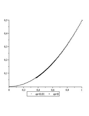
Figure 1: The minimizer (29) of Example 4.2 for fixed $\gamma=\nu=2$, $q=0.99$ and different values of $\omega$.

We note that in the limit, when $\gamma,\nu\rightarrow+\infty$, $\widetilde{y}(t)=\frac{1}{q+1}t^{2}+\frac{q}{q+1}t$ and coincides with the solution of the following problem with fixed initial and terminal points (cf. [20]):

$$\quad\mathcal{L}[y]=\int_{0}^{1}\left(y(qt+\omega)+\frac{1}{2}(D_{q,\omega}[y](t))^{2}\right)d_{q,\omega}t\longrightarrow\textrm{min}$$

subject to the boundary conditions

$$y(0)=0,\quad y(1)=1.$$

Expression $\gamma\frac{1}{2}(y(1)-1)^{2}+\nu\frac{1}{2}y^{2}(0)$ added to the Lagrangian $y(qt+\omega)+\frac{1}{2}(D_{q,\omega}[y](t))^{2}$ works like a penalty function when $\gamma$ and $\nu$ go to infinity. The penalty function itself grows, and forces the merit function (25) to increase in value when the constraints $y(0)=0$ and $y(1)=1$ are violated, and causes no growth when constraints are fulfilled. The minimizer (29) is represented in Figure 2 for fixed $q=0.5$, $\omega=1$ and different values of $\gamma$ and $\nu$.

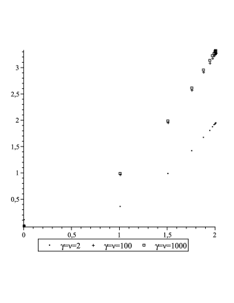
Figure 2: The minimizer (29) of Example 4.2 for fixed $q=0.5$, $\omega=1$ and different values of $\gamma$ and $\nu$.

Remark 4.3.

Let

$$\mathcal{L}[y]=\int_{0}^{1}\left(y(qt+\omega)+\frac{1}{2}(D_{q,\omega}[y](t))^{2}\right)d_{q,\omega}t$$

and

$$\widetilde{y}_{1}(t)=\frac{1}{q+1}t^{2}-\frac{\omega}{q+1}t+\frac{q+\omega}{q+1}\quad\mbox{and}\quad\widetilde{y}_{2}(t)=\frac{1}{q+1}t^{2}+\frac{q}{q+1}t.$$

Comparing Example 4.1 and Example 4.2, we can conclude that

$$\mathcal{L}[\widetilde{y}_{1}]<\mathcal{L}[\widetilde{y}_{2}].$$

In the next example we analyze an adjustment model in economics. For a deeper discussion of this model we refer the reader to [29].

Example 4.4.

Consider the dynamic model of adjustment

$$\mathcal{J}[y]=\sum_{t=1}^{T}r^{t}\left[\alpha(y(t)-\bar{y}(t))^{2}+(y(t)-y(t-1))^{2})\right]\longrightarrow\textrm{min},$$

where $y(t)$ is the output (state) variable, $r>1$ is the exogenous rate of discount and $\bar{y}(t)$ is the desired target level, and $T$ is the horizon. The first component of the loss function above is the disequilibrium cost due to deviations from desired target and the second component characterizes the agent s aversion to output fluctuations. In the continuous case the objective function has the form

$$\mathcal{J}[y]=\int_{1}^{T}e^{(r-1)t}\left[\alpha(y(t)-\bar{y}(t))^{2}+(y^{\prime}(t))^{2})\right]\longrightarrow\textrm{min}.$$

Let $q\in]0,1[$ and $\omega\geq 0$ be fixed real numbers, and $I$ be an interval of $\mathbb{R}$ such that $\omega_{0},0,T\in I$. The quantum model in terms of the Hahn operators which we wish to minimize is

$$\mathcal{J}[y]=\int_{0}^{T}E(1-r,t)\left[\alpha(y(qt+\omega)-\bar{y}(qt+\omega))^{2}+(D_{q,\omega}[y](t))^{2}\right]d_{q,\omega}t\longrightarrow\textrm{min},$$ (30)

where $E\left(z,\cdot\right)$ is the $q,\omega$-exponential function defined by

$$E\left(z,t\right):=\prod_{k=0}^{\infty}(1+zq^{k}(t(1-q)-\omega))$$

for $z\in\mathbb{C}$. Several nice properties of the $q,\omega$-exponential function can be found in [1, 2]. By Theorem 3.9, a solution to problem (30) should satisfy the following conditions

$$E(1-r,t)\left[\alpha(y(qt+\omega)-\bar{y}(qt+\omega))\right]=D_{q,\omega}\left[E(1-r,\cdot)D_{q,\omega}[y]\right](t),$$ (31)

for all $t\in\{\omega[n]_{q}:n\in\mathbb{N}_{0}\}\cup\{Tq^{n}+\omega[n]_{q}:n\in\mathbb{N}_{0}\}\cup\{\omega_{0}\}$; and

$$\left.E(1-r,t)D_{q,\omega}[y](t)\right|_{t=0}=0,\quad\left.E(1-r,t)D_{q,\omega}[y](t)\right|_{t=T}=0.$$ (32)

Taking the $q,\omega$-derivative of the right side of (31) and applying properties of the $q,\omega$-exponential function, for $t$ such that $|t-\omega_{0}|<\frac{1}{(r-1)(1-q)}$, we can rewrite (31) and (32) as

$$\left[1-(r-1)(t(1-q)-\omega)\right]\alpha(y(qt+\omega)-\bar{y}(qt+\omega))=(r-1)D_{q,\omega}[y](t)+D_{q,\omega}[D_{q,\omega}[y]](t),$$ (33)

$$\left.D_{q,\omega}[y](t)\right|_{t=0}=0,\quad\left.D_{q,\omega}[y](t)\right|_{t=T}=0.$$ (34)

Note that for $(q,\omega)\rightarrow(1,0)$ equations (33) and (34) reduce to

$$\alpha(y(t)-\bar{y}(t))=(r-1)y^{\prime}(t)+y^{\prime\prime}(t),$$

$$\left.y^{\prime}(t)\right|_{t=0}=0,\quad\left.y^{\prime}(t)\right|_{t=T}=0,$$

which are necessary optimality conditions for the continuous model.

5 Conclusions

In this paper we prove optimality conditions for quantum variational problems with a Lagrangian depending on the unspecified end-points $y(a)$, $y(b)$. Our approach uses the quantum derivative in the forward sense:

$$D_{q,\omega}\left[f\right]\left(t\right):=\frac{f\left(qt+\omega\right)-f\left(t\right)}{\left(q-1\right)t+\omega},\quad t\neq\omega_{0}$$

where $q\in]0,1[$ and $\omega\geq 0$, which corresponds to the delta approach in the time scale context. However, sometimes with respect to applications (see [6, 7, 22, 21]) the backward approach is preferable. In this sense the quantum operator

$$D_{q,\omega}\left[f\right]\left(t\right):=\frac{f\left(qt+\omega\right)-f\left(t\right)}{\left(q-1\right)t+\omega},\quad t\neq\omega_{0}$$

where $q\in]0,1[$ and $\omega<0$, could be considered. Other interesting open question consists of finding a solution of equation (33). As we have observed choosing particular values of $r$, $\alpha$, and a target function, a numerical method should be used in order to solve the Euler-Lagrange equation for the problem in Example 4.4. Those issues need to be examined further and will be considered in the future.

References

- [1] K. A. Aldwoah, Generalized time scales and associated difference equations, PhD thesis, Cairo University, 2009.
- [2] K. A. Aldwoah and A. E. Hamza, Difference time scales, Int. J. Math. Stat. 9 (2011), no. A11, pp. 106–125.
- [3] R. Almeida and D. F. M. Torres, Isoperimetric problems on time scales with nabla derivatives, J. Vib. Control 15 (2009), pp. 951–958. arXiv:0811.3650
- [4] R. Almeida and D. F. M. Torres, Hölderian variational problems subject to integral constraints J. Math. Anal. Appl. 359 (2009), no. 2, pp. 674–681. arXiv:0807.3076
- [5] R. Álvarez-Nodarse, On characterizations of classical polynomials, J. Comput. Appl. Math. 196 (2006), no. 1, pp. 320–337.
- [6] F. M. Atici and F. Uysal, A production-inventory model of HMMS on time scales, Appl. Math. Lett. 21 (2008), no. 3, pp. 236–243.
- [7] F. M. Atici and C. S. McMahan, (2009) A comparison in the theory of calculus of variations on time scales with an application to the Ramsey Model, Nonlinear Dyn. Syst. Theory 9 (2009), no. 1, pp. 1–10.
- [8] B. Aulbach and S. Hilger,(1990) A unified approach to continuous and discrete dynamics, in: em Qualitative theory of differential equations, B. Sz-Nagy and L. Hatvani, eds., North-Holland, Amsterdam, 1990, pp. 37–56.
- [9] Z. Bartosiewicz, N. Martins and D. F. M. Torres, The second Euler-Lagrange equation of variational calculus on time scales, Eur. J. Control 17 (2011), no. 1, pp. 9–18. arXiv:1003.5826
- [10] A. M. C. Brito da Cruz, and N. Martins and D. F. M. Torres, Higher-order Hahn’s quantum variational calculus, Nonlinear Anal. 75 (2012), no. 3, 1147–1157. arXiv:1101.3653
- [11] M. R. Caputo, Foundations of Dynamic Economic Analysis: Optimal Control Theory and Applications, Cambridge University Press, Cambridge, 2005.
- [12] P. A. F. Cruz, D. F. M. Torres and A. S. I. Zinober, A non-classical class of variational problems, Int. J. Mathematical Modelling and Numerical Optimisation 1 (2010), no. 3, pp. 227–236. arXiv:0911.0353
- [13] A. Dobrogowska and A. Odzijewicz, Second order -difference equations solvable by factorization method, J. Comput. Appl. Math. 193 (2006), no. 1, pp. 319–346. arXiv:math-ph/0312057
- [14] T. Ernst, The different tongues of -calculus, Proc. Est. Acad. Sci. 57 (2008), no. 2, pp. 81–99.
- [15] R. A. C. Ferreira and D. F. M. Torres Higher-order calculus of variations on time scales, in Mathematical control theory and finance, Springer, Berlin, 2008, pp. 149–159. arXiv:0706.3141
- [16] R. A. C. Ferreira, A. B. Malinowska and D. F. M. Torres, Optimality conditions for the calculus of variations with higher-order delta derivatives, Appl. Math. Lett. 24 (2011), no. 1, pp. 87–92. arXiv:1008.1504
- [17] W. Hahn, Über Orthogonalpolynome, die -Differenzengleichungen genügen, Math. Nachr. 2 (1949), pp. 4–34.
- [18] K. Kaivant and A. Zinober, Optimal production subject to piecewise continuous royalty payment obligations, submitted.
- [19] A. B. Malinowska and D. F. M. Torres, Natural boundary conditions in the calculus of variations, Math. Methods Appl. Sci. 33 (2010), pp. 1712–1722, DOI:10.1002/mma.1289. arXiv:0812.0705
- [20] A. B. Malinowska and D. F. M. Torres, The Hahn quantum variational calculus, J. Optim. Theory Appl. 147 (2010), no. 3, pp. 419–442, DOI: 10.1007/s10957-010-9730-1. arXiv:1006.3765
- [21] A. B. Malinowska and D. F. M. Torres, A general backwards calculus of variations via duality, Optim. Lett. 5 (2011), no. 4, 587–599. arXiv:1007.1679
- [22] A. B. Malinowska and D. F. M. Torres, Backward variational approach on time scales with an action depending on the free endpoints, Z. Naturforsch. A 66a (2011), no. 6, 401–410. arXiv:1101.0694
- [23] A. B. Malinowska, N. Martins and D. F. M. Torres, Transversality conditions for infinite horizon variational problems on time scales, Optim. Lett. 5 (2011), no. 1, pp. 41–53. arXiv:1003.3931
- [24] N. Martins and D. F. M. Torres, Calculus of variations on time scales with nabla derivatives, Nonlinear Anal. 71 (2009), no. 12, pp. e763–e773. arXiv:0807.2596
- [25] N. Martins and D. F. M. Torres, Noether’s symmetry theorem for nabla problems of the calculus of variations, Appl. Math. Lett. 23 (2010), pp. 1432–1438, DOI: 10.1016/j.aml.2010.07.013. arXiv:1007.5178
- [26] N. Martins and D. F. M. Torres, Generalizing the variational theory on time scales to include the delta indefinite integral, Comput. Math. Appl. 61 (2011), no. 9, 2424–2435. arXiv:1102.3727
- [27] V. Kac and P. Cheung, Quantum calculus, Springer, New York, 2002.
- [28] J. Petronilho, Generic formulas for the values at the singular points of some special monic classical -orthogonal polynomials, J. Comput. Appl. Math. 205 (2007), no. 1, pp. 314–324.
- [29] J. K. Sengupta, Recent models in dynamic economics: problems of estimating terminal conditions, Int. J. Syst. Sci. 28, (1997), pp. 857–864.
- [30] B. van Brunt, The calculus of variations, Springer, New York, 2004.