Robust Hedging of Withdrawal Guarantees
(Extended Version)

Abstract

Withdrawal guarantees ensure the periodical deduction of a constant dollar-amount from a fund investment for a fixed number of periods. If the fund depletes before the last withdrawal, the guarantor has to finance the outstanding withdrawals. We derive a robust hedging strategy which leads to closed form solutions for the guarantee value.

1 Introduction

In the life insurance industry, withdrawal guarantees have emerged during the last decades as a guarantee feature in variable annuity products. In typical withdrawal guarantee products, so-called guaranteed minimum withdrawal benefit (GMWB) policies, the initial annuitization amount is invested into a fund (mostly with a significant equity component) and then fixed withdrawal payments are periodically deducted from the fund. These periodical withdrawals are guaranteed up to a specified maturity; if the fund depletes beforehand, the guarantor has to finance the outstanding withdrawal payments. See [1, 6] and the references therein for further details on GMWB products.

The withdrawal process is conceptually different from consumption models in standard portfolio optimization approaches, see e.g. [4], where a constant fraction of the current fund value is permanently consumed. The latter consumes less when the fund value has decreased and more when the fund has outperformed. Withdrawal guarantee products, on the contrary, always consume the same absolute dollar-amount, which leads to a fundamentally different kind of path dependency.

This paper analyzes semi-static hedging strategies for withdrawal guarantees and uses heavily techniques from static hedging theory, which was originated by Breeden and Litzenberger [2] and has been further developed by Carr et al. [3]. The hedging strategies consist in rolling over portfolios of short-dated put options with different strikes but with common maturity equal to the subsequent withdrawal time. The hedge portfolios are constructed to finance either all outstanding withdrawals if the fund depletes or otherwise the roll-over into the new hedge portfolio of short-dated put options.

If the market dynamics (here the underlying asset price) is driven by a one-factor Markov process, the semi-static hedging strategy leads to a perfect replication. This applies in particular for the local volatility model. We show how the weights of the single put options with specific strikes in the hedging portfolio can be derived backward recursively.

If an additional stochastic market factor comes into play, such as stochastic volatility, then the semi-static hedging strategy becomes sensitive with respect to moves in this additional factor. Hence the replication might not be perfect. We analyze in a Black-Scholes setting the forward vega and volga sensitivities of the withdrawal guarantee after forward vega hedge and discover a long volga position if the guarantee is not too far out-of- or in-the-money. Hence, any move of the forward volatility works in favor of the hedger. As stochastic volatility models account for systematic hedging gains due to the volatility of volatility, they are expected to value at-the-money withdrawal guarantees at a lower price and vice versa if the guarantee is far out-of- or in-the-money case. This expectation is verified for the Heston model by comparing it against the local volatility model.

If the asset price process has independent returns, i.e. is of exponential Lévy type, the expressions for the withdrawal guarantee value and the option weights in the semi-static hedging strategy simplify considerably. We show that the option weights for the different time steps can be represented as density of a process that evolves backwards in time. This process is identified as value process of a multi-contribution fund to which constant money amounts are periodically contributed (rather than deducted as in the withdrawal fund case). This fund is driven by an asset process that is reverse $\Gamma$-adjoint to the underlying asset process of the withdrawal guarantee. The withdrawal guarantee value can then be represented as a call option on the adjoint multi-contribution fund. The duality between withdrawal guarantee and multi-contribution fund also holds vice versa: a put option on a multi-contribution fund is semi-statically hedgeable and can be interpreted as a call option on the adjoint withdrawal fund.

We also show that the static hedging representation can be extended to withdrawal guarantees with roll-up feature (also known as ratchet feature) that increases the guaranteed withdrawal level when the fund has outperformed.

The paper is organized as follows: section 2 gives a more detailed description of withdrawal guarantees. In section 3, the main ideas for deriving the static hedging strategy are outlined for the simple two-period case and the effects of stochastic volatility are analyzed. Section 4 generalizes for the multi-period case, exhibits the duality between withdrawal guarantees and multi-contribution funds and extends to the roll-up case.

2 Formalizing the Withdrawal Guarantee

We denote by $X_{0}$ the initial capital (i.e. the initial annuity reserve) which is invested into an asset with price process $(S_{t})_{t\geq 0}$. Let $0=T_{0}<T_{1}<\dots<T_{N}=T^{*}$ denote the schedule of withdrawal times with maturity $T^{*}$ and equidistant time intervals $\Delta T:=T^{*}/N$. At each time $T_{t}$, the fixed withdrawal amount $w>0$ is deducted from the fund. We denote by $X_{t}$ the fund value at withdrawal time $T_{t}$, $t=1,\dots,N$, after the withdrawal amount has been deducted. Analogously, we write short-hand $S_{t}$ for the asset price at time $T_{t}$, and we assume for simplicity $S_{0}=1$ for the initial asset price.

The fund value process obeys the obvious recursion relation

$$X_{t+1}=X_{t}\cdot S_{t+1}/S_{t}-w\,,\qquad t=0,\dots,N-1\,.$$ (1)

Iterating the recursion yields

$$X_{t}=S_{t}\cdot\left(X_{0}-w\cdot\sum_{u=1}^{t}\frac{1}{S_{u}}\right)=S_{t}\cdot\left(X_{0}-\varpi\cdot\sum_{u\,:\,0<T_{u}\leq T_{t}}\frac{\Delta T}{S_{u}}\right)\qquad(t=1,\dots,N)\,,$$ (2)

where $\varpi$ denotes the annualized withdrawal rate, i.e. $\varpi=w/\Delta T$. The sum expression is known as the harmonic average functional of the asset price $S$.

The withdrawal guarantee works as follows: the withdrawal payments until maturity $T^{*}$ are guaranteed to the investor (or policy holder) even if the fund depletes before $T^{*}$. In this case, the guarantor must finance the outstanding withdrawals.

We denote by $\tau$ the depletion time of the fund, which is the first time when the fund value is not sufficient to finance the current withdrawal amount $w$, i.e. $\tau:=\inf\{t:X_{t}\leq 0\}$.

The total withdrawal guarantee can be decomposed into contingent guarantee claims $Z^{(t)}$, $t=1,\dots,N$. The single claim $Z^{(t)}$ is due at withdrawal time $T_{t}$ and can be expressed as follows: if the fund is already depleted before time $T_{t}$, the guarantor has to finance the complete withdrawal amount $w$. If the ruin of the fund happens at time $T_{t}$, the guarantor has to pay only that part of $w$ that can no more be financed by the fund, i.e. the negative part $X_{t}^{-}:=-\min(0,X_{t})$ of the fund value $X_{t}$ after withdrawal of the full amount $w$. Hence, $Z^{(t)}$ can be written as

$$Z^{(0)}=0\,,\qquad Z^{(t)}=w\cdot{\rm\bf 1}_{\tau\leq t-1}+X_{t}^{-}\cdot{\rm\bf 1}_{\tau=t}\,,\qquad t=1,\dots,N\,.$$ (3)

Here, ${\rm\bf 1}_{\tau=t}$ denotes the indicator function of the set $\{\tau=t\}$. The contingent guarantee payments are visualized in figure 1.

[Figure 1 should be inserted here]

For simplicity reasons, we assume zero interest rates. If the market consistent pricing measure is given by the equivalent martingale measure ${\mathbb{Q}}$, then the market value $V_{t}$ at time $T_{t}$ of all guarantee claims payable at time $T_{t}$ or later reads

$$V_{t}:={\mathbb{E}}_{t}^{\mathbb{Q}}\left[\sum_{u=t}^{N}Z^{(u)}\right]\,,\qquad t=0,\dots,N\,,$$ (4)

where ${\mathbb{E}}_{t}^{\mathbb{Q}}$ denotes conditional expectation with respect to the filtration ${\mathcal{F}}_{t}$ which contains all probability information observed until time $T_{t}$.

By inspection of (3) the value $V_{0}$ at time $T_{0}$ of the total withdrawal guarantee can also be written as

$$V_{0}={\mathbb{E}}^{\mathbb{Q}}[w\cdot(N-\tau)^{+}+X_{\tau}^{-}\cdot{\rm\bf 1}_{\tau\leq N}]\,,$$

and reads essentially as a put option on the depletion time $\tau$.

Multi-Contribution Fund and Continuous Time Limit

The withdrawal guarantee is closely related to the dynamics of a multi-contribution fund $Y$ on an underlying asset $\tilde{S}$, to which a constant money amount $p>0$ is periodically contributed. If the schedule of contributions coincides with that of the withdrawal case, $Y$ follows a recursion relation analog to (1)

$$Y_{0}:=p\,,\qquad Y_{t+1}=Y_{t}\cdot\tilde{S}_{t+1}/\tilde{S}_{t}+p\quad(t=0,\dots,N-1)\,.$$ (5)

Iterating this recursion yields

$$Y_{t}=\pi\cdot\tilde{S}_{t}\cdot\sum_{u=0}^{t}\frac{\Delta T}{\tilde{S}_{u}}\,,$$ (6)

where $\pi$ denotes the annualized contribution rate, i.e. $\pi=p/\Delta T$.

In the continuous time limit, the number of withdrawals $N$ tends to infinity and $\Delta T\to 0$. It follows immediately from (2) that the withdrawal fund process $X$ and the multi-contribution fund process $Y$ converge to the processes

$$\bar{X}_{T}=S_{T}\cdot\left(X_{0}-\varpi\int_{0}^{T}\frac{du}{S_{u}}\right)\,,\quad\bar{Y}_{T}=\pi\cdot\tilde{S}_{T}\cdot\int_{0}^{T}\frac{du}{\tilde{S}_{u}}\qquad(0\leq T\leq T^{*})\,.$$ (7)

The recursion relations (1) and (5) translate into the Itô differential equations $d\bar{X}_{t}=\frac{\bar{X}_{t}}{S_{t}}\,dS_{t}-\varpi\,dt$ and $d\bar{Y}_{t}=\frac{\bar{Y}_{t}}{\tilde{S}_{t}}\,d\tilde{S}_{t}+\pi\,dt$, respectively.

Further notations: $X_{t-}:=X_{t}+w$ denotes the fund value at time $T_{t}$ before deduction of the withdrawal. Setting $\zeta_{t}:=X_{t}/S_{t}$, we obtain $X_{t}=\zeta_{t-1}S_{t}-w$ and $\zeta_{t}=\zeta_{t-1}-w/S_{t}$ by the recursion relation (1). We denote by $P_{t,t^{\prime}}(K)$ the (forward) value of a vanilla put option on $S$ at time $T_{t}$ with maturity $T_{t^{\prime}}$ and strike $K$. If $T_{t^{\prime}}=T_{t+1}$, we write $P_{t}(K)$. When we wish to emphasize the dependence of the option value on the spot value $S_{t}$, we write $P_{t}(K|\,S_{t})$. We denote by $\Delta_{t}(K|S_{t})$ the first and by $\Gamma_{t}(K|S_{t})$ the second derivative of the put $P_{t}(K|S_{t})$ with respect to the spot $S_{t}$, the first and second derivative in strike dimension is denoted by $\partial_{\mathcal{K}}P_{t}(K)$ and $\partial_{\mathcal{K}}^{2}P_{t}(K)$.

3 The Two-Period Case

We illustrate the main ideas of hedging withdrawal guarantees in the two-period case when only two withdrawals are guaranteed at times $T_{1}$ and $T_{2}$.

We can rewrite the claim $Z^{(1)}$ due at time $T_{1}$ as follows

$$Z^{(1)}=X_{1}^{-}=-\min\left(0,\zeta_{0}S_{1}-w\right)=\zeta_{0}\left(w/\zeta_{0}-S_{1}\right)^{+}\,.$$ (8)

Hence $Z^{(1)}$ could be perfectly hedged as of time $T_{0}$ by purchasing $\zeta_{0}$ units of the put $P_{0}(w/\zeta_{0})$.

Hedging the claim $Z^{(2)}$ due at time $T_{2}$ in addition to $Z^{(1)}$ is more challenging. We will work backwards in time. At time $T_{1}$, the asset price $S_{1}$ and hence also the fund value $X_{1}$ is known. In particular, it is clear whether the fund is already depleted or not. Depletion has happened if $X_{1}<0$, or equivalently $S_{1}<w/\zeta_{0}$. In this case, the guarantor knows that they need to pay $w-\zeta_{0}S_{1}$ at time $T_{1}$ and one period later, at $T_{2}$, the full withdrawals amount $w$, in total the amount $2w-\zeta_{0}S_{1}$. If the fund is not depleted, the guarantor must buy protection for the case that the fund at time $T_{2}$ can not fully finance the second withdrawal. This protection consists in purchasing $\zeta_{1}$ units of the put $P_{1}(w/\zeta_{1}|S_{1})$ at time $T_{1}$ which follows from rewriting the claim $Z^{(2)}$ analogously to (8).

Hence the value $V_{1}$ at time $T_{1}$ of the outstanding guarantee claims, i.e. the costs to finance $Z^{(1)}$ and the protection against $Z^{(2)}$ one period later, can be summarized as

$$V_{1}=\left\{\begin{array}[]{lll}2w-\zeta_{0}S_{1}&&\mbox{if }S_{1}\leq w/\zeta_{0}\,,\\ \zeta_{1}P_{1}\left(w/\zeta_{1}|S_{1}\right)=(\zeta_{0}-\frac{w}{S_{1}})\cdot P_{1}\left(\frac{w}{\zeta_{0}-\frac{w}{S_{1}}}\,\big{|}\,S_{1}\right)&&\mbox{if }S_{1}>w/\zeta_{0}\,.\\ \end{array}\right.$$ (11)

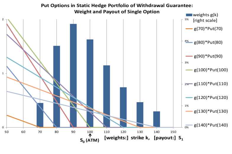
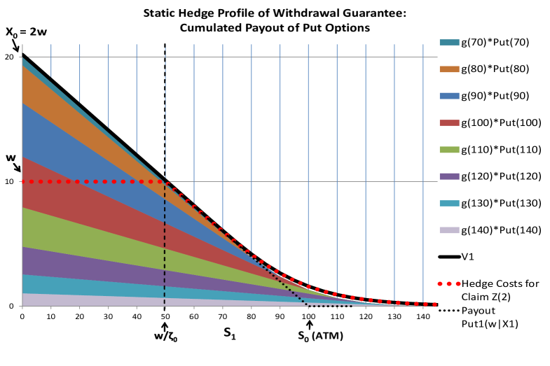
Figure 2: Discrete version of the static hedge portfolio for the two-period withdrawal guarantee in a Black-Scholes setting with volatility set to $0.25$. Top: weights $g(k)$ of the single put option $P_{0}(k)$ and payout profile of the weighted options. Bottom: cumulated payout of the weighted put options, which matches closely the profile of the hedging costs $V_{1}=V_{1}(S_{1})$ at time $T_{1}$ (black solid line). The red dotted line shows only that part of $V_{1}$ which corresponds to the hedging costs for the claim $Z^{(2)}$.

The function $V_{1}$ is visualized by the black solid line in the bottom graph of figure 2. The red dotted line shows only that part of $V_{1}$ which corresponds to the hedging costs at time $T_{1}$ for the claim $Z^{(2)}$. Note that the function $V_{1}$ is continuous at $S_{1}=w/\zeta_{0}$.

[Figure 2 should be inserted here]

Static Hedging

The withdrawal guarantee would be perfectly hedged if the costs for the put option in $V_{1}$ could be locked in at time $T_{0}$ already. However, it is generally not possible to perfectly hedge the forward put $P_{1}(w/\zeta_{1}\,|S_{1})$ as of today using vanilla hedging instruments, since the put depends on the future implied volatility at time $T_{1}$ with moneyness $(w/\zeta_{1})/S_{1}=w/X_{1}$, which is not fixed before time $T_{1}$.

If the value of the forward put at time $T_{1}$ depends only on the asset price $S_{1}$, then classical static hedging theory can be applied.

Let us recall the famous Breeden-Litzenberger formula: the risk neutral density of the asset price $S_{1}$ can be inferred from market quotes by differentiating vanilla put option prices twice with respect to the strike, i.e. ${\mathbb{Q}}(S_{1}\in dk)=\partial_{\mathcal{K}}^{2}P_{0}(k)dk$. Hence, any European option with payout $\phi(S_{1})$ at time $T_{1}$ can be statically hedged by a portfolio of vanilla put options with different strikes. If the function $\phi$ is twice differentiable, the static hedge portfolio is obtained by applying twice partial integration on the option value:

$${\mathbb{E}}^{\mathbb{Q}}[\phi(S_{1})] = \int_{0}^{\infty}\phi(k)\,{\mathbb{Q}}(S_{1}\in dk)=\int_{0}^{\infty}\phi(k)\,\partial_{\mathcal{K}}^{2}P_{0}(k)dk$$ (12)

$$= \left[\phi(k)\partial_{\mathcal{K}}P_{0}(k)\right]_{k=0}^{\infty}-\left[\phi^{\prime}(k)P_{0}(k)\right]_{k=0}^{\infty}+\int_{0}^{\infty}\phi^{\prime\prime}(k)\,P_{0}(k)dk\,.$$

To ensure the prerequisites for static hedging, the following assumptions are imposed on the asset price process, which are formulated in the more general multi-period setting:

(A1)

$(S_{t})_{t\geq 0}$ is a one-factor Markov process and every $S_{t}$ is continuously distributed.

Clearly, all one-dimensional diffusion models for the asset price dynamics (Black-Scholes, Dupire’s local volatility model, etc.) satisfy assumption (A1). The same is true for one-dimensional exponential Lévy models (such as Merton’s jump diffusion, variance gamma, normal inverse Gaussian or CGMY model), see [7] for references and further details. Note that assumption (A1) rules out stochastic volatility models.

The Markov property implies that forward put options at time $T_{t}$ written on $(S_{t})_{t\geq 0}$ depend only on the state of the market at time $T_{t}$ and hence only on the spot $S_{t}$ which is the unique market factor. Further, the regularity assumption implies that the put values $P_{t}(K|S_{t})$ are twice differentiable with respect to strike $K$ (and spot $S_{t}$) for every $t=0,\dots,N-1$.

Assumption (A1) ensures that ${V}_{1}$ depends only on the asset price $S_{1}$ at time $T_{1}$. Hence the static hedging formula (12) can be applied to the function ${V}_{1}={V}_{1}(S_{1})$. We obtain the hedging strategy that locks in the guarantee costs $V_{1}$ already as of time $T_{0}$ and hence perfectly replicates the withdrawal guarantee.

The following technical smoothness and boundary conditions on the function $V_{1}$ and its first derivative $V_{1}^{\prime}:=\partial_{S_{1}}V_{1}$ guarantee that the boundary terms in the static hedging formula (12) vanish (the proof of these conditions has been transferred to the appendix):

$${V}_{1} {V}_{1}^{\prime} w/\zeta_{0}$$ and are continuous at and take the following boundary values: (13)

	${V}_{1}(k)$	${V}_{1}^{\prime}(k)$
$k=0$	$2w$	$-1$
$k\to\infty$	$0$	$o(1/k)$

This condition implies that all boundary terms in the static hedging formula (12) vanish when we recall the boundary behavior of the put option $P_{0}(0)=0$ and $P_{0}(k)\sim k$, $\partial_{\mathcal{K}}P_{0}(k)\to 1$ as $k\to\infty$.

Keeping in mind that the function ${V}_{1}$ is linear on the interval $[0,w/\zeta_{0}]$ with zero second order derivative, the static hedging formula (12) leads to the following result:

Under assumption (A1), the two-period withdrawal guarantee can be perfectly hedged as of time $T_{0}$ by the portfolio

$$V_{0}=\int_{w/\zeta_{0}}^{\infty}\gamma(k)\,P_{0}(k)dk$$ (14)

of put options $P_{0}(k)$ with common maturity $T_{1}$ but different strikes $k>0$ that are weighted according to the function

$$\gamma(k):=V_{1}^{\prime\prime}(k)=\left[D_{S_{1}}^{2}\left\{\left(\mbox{$\zeta_{0}-\frac{w}{S_{1}}$}\right)\cdot P_{1}\Big{(}\frac{w}{\zeta_{0}-\frac{w}{S_{1}}}\,\big{|}\,S_{1}\Big{)}\right\}\right]_{S_{1}=k}\,,\qquad k>w/\zeta_{0}\,.$$ (15)

The value of the two-period withdrawal guarantee at time $T_{0}$ is hence given by $V_{0}$.

A discrete real-world version of the static hedge portfolio in a Black-Scholes setting is visualized in figure 2. The top graph displays the weights of the single put option $P_{0}(k)$ for strikes according to moneyness levels from $0.7$ to $1.4$, together with the payout profile of the correctly weighted put options. The lower graph shows the cumulated payout of the weighted put options and demonstrates that it matches closely the hedging costs $V_{1}$ at time $T_{1}$.

One-factor Exponential Lévy Case

The static hedging representation simplifies significantly if we assume that the asset-price process has independent returns, i.e. $S_{t+1}/S_{t}$ is independent of $S_{t}$ for every $t=1,\dots,N$. This assumption is equivalent to the following scaling property

(A2)

$P_{t}(\alpha K|\alpha S_{t})=\alpha P_{t}(K|S_{t})$ for every $\alpha>0$ and every $t=0,\dots,N-1$ and $K>0$.

Of course, one-factor exponential Lévy models satisfy this assumption. We do not need the assumption of stationary returns; e.g. a Black-Scholes model with deterministic time-dependent volatility would also be allowed.

Under assumption (A2), the function $V_{1}$ in (11) collapses to $V_{1}(S_{1})=P_{1}\left({w}\,|\,\zeta_{0}S_{1}-{w}\right)$ for $S_{1}>w/\zeta_{0}$. Hence the weight function $\gamma$ in (15) can be rewritten:

$$\gamma(k)=V_{1}^{\prime\prime}(k)=\zeta_{0}^{2}\cdot\Gamma_{1}\left({w}\,|\,\zeta_{0}k-{w}\right)=\zeta_{0}^{2}\cdot g\left(\zeta_{0}k\right)\,,\qquad k>w/\zeta_{0}\,,$$

with function $g$ defined as

$$g\left(k^{\prime}\right):=\Gamma_{1}\left({w}\,|\,k^{\prime}-{w}\right)\,,\qquad k^{\prime}>w\,.$$ (16)

Under the additional assumption (A2), the hedge portfolio for the two-period withdrawal guarantee in (14) hence simplifies as follows (when applying a change of integration variable $k^{\prime}=\zeta_{0}k$):

$$V_{0} = \int_{w/\zeta_{0}}^{\infty}\zeta_{0}^{2}\cdot g\left(\zeta_{0}k\right)\cdot P_{0}(k\,|\,S_{0})\,dk=\int_{w}^{\infty}g(k^{\prime})\cdot P_{0}(k^{\prime}\,|\,X_{0})\,dk^{\prime}\,.$$ (17)

Effects of Stochastic Volatility

It is evident from the perfect static hedging replication in (17) that the sensitivity of the withdrawal guarantee with respect to instantaneous shocks of the asset price (delta and gamma) stems exclusively from the portfolio of short-term put options $P_{0}(k)$, whereas the weight function $g$ does not contribute. The story is different for the sensitivity with respect to volatility shocks (vega). While the short-term vega stemming from shocks of the implied volatility with maturity $T_{1}$ is statically hedged by the portfolio of short-term puts $P_{0}(k)$, the forward put $P_{1}(w/\zeta_{1}\,|\,S_{1})$ and hence the weight function $g$ depend on the $T_{1}$-in-$T_{2}$-forward volatility $\Sigma_{1}$, which leads to a forward-vega exposure.

If the volatility is allowed to be stochastic, i.e. if the assumption (A1) is dropped, the forward-vega exposure from the weight function $g$ must also be hedged. It is intuitive to hedge this exposure with a $T_{1}$-in-$T_{2}$-forward variance swap which is only sensitive with respect to the forward volatility $\Sigma_{1}$.

The variance swap hedge is constructed to offset the first-order sensitivity of the withdrawal guarantee with respect to changes in forward volatility, but the second order forward volatility sensitivity (known as vega-gamma or volga) of the net position after hedge does not necessarily vanish. When forward volatility moves, a long volga net position works in favor of the hedger and a short volga position would produce systematic losses. Since stochastic volatility models typically account for these systematic gains or losses, they are expected to produce higher model values for guarantees with dominant short volga net position and vice versa for a long volga position.

In the remaining part of this section, we analyze in a Black-Scholes setting the volga position of the withdrawal guarantee after the forward variance swap hedge and observe long and short volga positions depending on the moneyness. We will then compare these findings with the Heston model. In particular, we analyze for different moneyness levels of the withdrawal guarantee the model value differences of the Heston and the corresponding local volatility model.

In the Black-Scholes world, the forward-vega $\partial_{\Sigma_{1}}V_{0}$ and forward-volga exposure $\partial_{\Sigma_{1}}^{2}V_{0}$ of the withdrawal guarantee can be expressed in terms of Black-Scholes formulae by means of equations (16) and (17). The forward-vega exposure of the hedge with $T_{1}$-in-$T_{2}$-forward variance swaps must match the exposure of the withdrawals guarantee, i.e. must be equal to $\partial_{\Sigma_{1}}V_{0}$. Since the payout of a variance swap is quadratic in volatility, its vega is linear in volatility and volga is constant and equals $\mbox{vega}\,/\,\mbox{volatility}$. Hence the forward-volga of the forward variance swap hedge for the withdrawal guarantee is given by $\partial_{\Sigma_{1}}V_{0}/\Sigma_{1}$ and the forward-volga of the net position after hedge reads $\partial_{\Sigma_{1}}V_{0}/\Sigma_{1}-\partial_{\Sigma_{1}}^{2}V_{0}$.

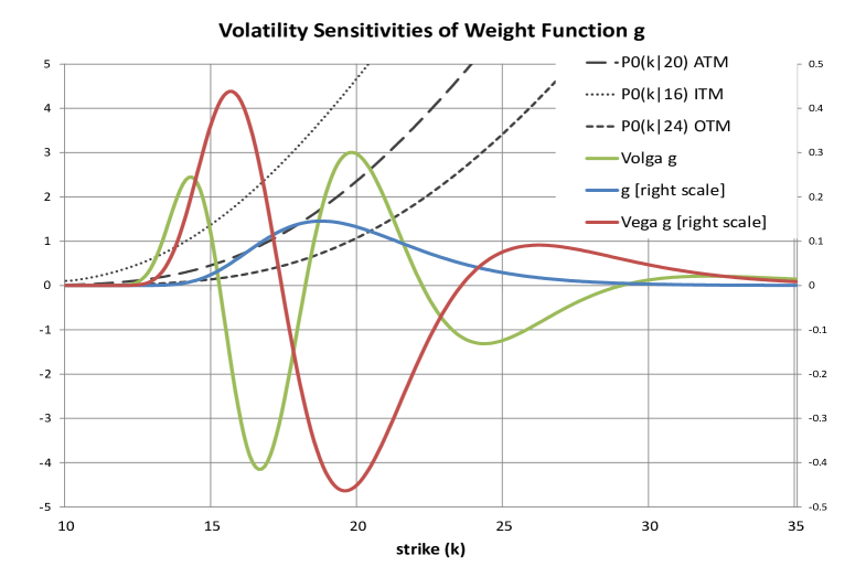
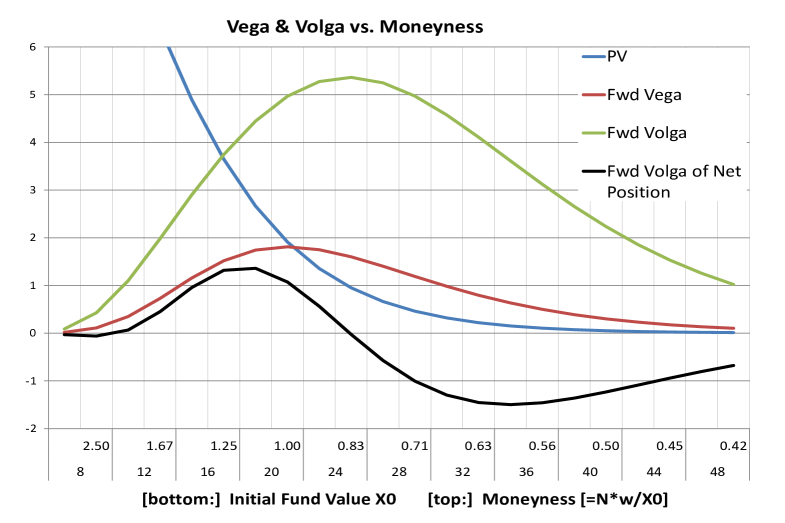
Figure 3: The top graph shows the weight function $g$ in the representation of the two-period withdrawal guarantee and its sensitivities (vega and volga) with respect to the $T_{1}$-$T_{2}$-forward volatility. Additionally, put values as a function of strike for different initial fund values are shown. Integrating the weight function or its volatility sensitivities against the put value functions gives the corresponding withdrawal guarantee values, which are shown in the bottom graph for different moneyness levels. In addition, the volga of the net position after hedge with forward starting variance swap is shown. Setting: Black-Scholes model with volatility $=0.3$, zero interest rates and dividends; withdrawal amount $w=10$.

[Figure 3 should be inserted here]

In the top graph in figure 3, the weight function $g$ defined in (16) is displayed together with its first and second derivative $\partial_{\Sigma_{1}}g$ and $\partial_{\Sigma_{1}}^{2}g$ with respect to the forward volatility $\Sigma_{1}$. As outlined in (17), we obtain the present value as well as the forward-vega and forward-volga exposure of the withdrawal guarantee by integrating these functions against the initial put prices $k\mapsto P_{0}(k|X_{0})$. The bottom graph in figure 3 visualizes these values for different initial fund values or moneyness levels, respectively, together with the volga of the net position after hedge. A long volga net position is observed for moneyness levels in a wide range around the at-the-money case. In the extreme out-of-the-money case, when the sum of the guaranteed amounts is less than ca. 70% of the initial capital, a short volga position shows up.

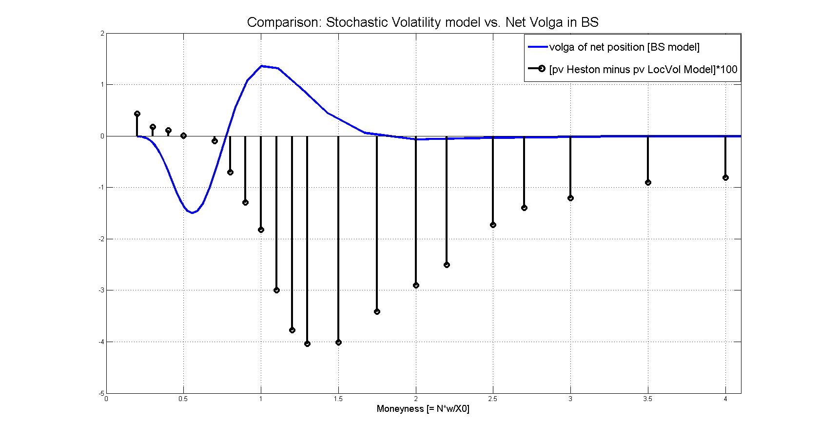
Figure 4: For the two-period withdrawal guarantee, the graph displays how the difference between Heston and local volatility model value depends on the moneyness of the guarantee and compares this dependence with the volga of the net position after hedge in the Black-Scholes setting. The Heston model value is below the local volatility model value mainly for those moneyness levels that show a long volga net position in the Black Scholes setting; vice versa for moneyness levels with short volga net position. The Heston model parameters are as follows: initial and long-term vol $=26.5\%$, mean reversion $=1.0$, vol-of-vol $=0.8$ and spot-vol-correlation $=0$. The local volatility model is calibrated to fit the Heston model value of the vanilla option market. The Black-Scholes setting for the net volga corresponds to that of figure 3.

[Figure 4 should be inserted here]

Figure 4 shows the model value differences of the Heston model and the corresponding local volatility model and compares these differences to the above volga analysis. As expected, the region of moneyness levels where the Heston model values are below the local volatility model values coincides approximately with the long volga region for the net position after hedge in the Black-Scholes setting; vice versa for the short volga region.

4 Multi-Period Setting

We extend the semi-static hedging hedging techniques to the multi-period case with guaranteed withdrawals at times $T_{1},\dots,T_{N}$.

General One-Factor Markov Case

Assuming (A1), we analyze the costs ${V}_{t}$ for settling the claim $Z^{(t)}$ at time $T_{t}$ and setting up the hedging costs for claims occurring later than $T_{t}$.

Applying the tower law for conditional expectation to definition (4) of $V_{t}$, we obtain the recursion relation

$$V_{t}=Z^{(t)}+{\mathbb{E}}_{t}^{\mathbb{Q}}[V_{t+1}]\qquad(t=0,\dots,N-1)\,.$$ (18)

Together with the recursion (1) of the fund value $X_{t}$, we deduce that the process $V$ is Markovian and that $V_{t}$ depends only on $X_{t}$ and $S_{t}$ or, equivalently, on $\zeta_{t-1}$ and $S_{t}$, i.e. $V_{t}=V_{t}(S_{t}\,|\,\zeta_{t-1})$. In addition, the propagation from $V_{t}$ to $V_{t+1}$ is fully specified by the one-period return $S_{t+1}/S_{t}$ of the underlying. Hence, if the fund does not deplete at time $T_{t}$, i.e. $\tau>t$, the conditional expectation in (18) can be written as

$${\mathbb{E}}_{t}^{\mathbb{Q}}[V_{t+1}]=\int_{0}^{\infty}V_{t+1}(k\,|\,\zeta_{t}=\zeta_{t-1}-w/S_{t})\,{\mathbb{Q}}(S_{t+1}\in dk|S_{t})\,.$$ (19)

If we now condition separately on the events $\{\tau<t\}$, $\{\tau=t\}$, and $\{\tau>t\}$ as in (11) and apply the same static hedging technique to (19) as in the two-period case, we arrive at the following backwards relation: for $t=0,\dots,N-2$,

$${V}_{t}(S_{t}\,|\,\zeta_{t-1})={\rm\bf 1}_{\tau<t}\cdot(N-t+1)w$$

$$+{\rm\bf 1}_{S_{t}\leq{w}/{\zeta_{t-1}}}\cdot\Big{[}(N-t+1)w-\zeta_{t-1}S_{t}\Big{]}$$

$$+{\rm\bf 1}_{S_{t}>{w}/{\zeta_{t-1}}}\cdot\int_{\frac{w}{\zeta_{t-1}-\frac{w}{S_{t}}}}^{\infty}P_{t}(k\,|\,S_{t})\cdot\left[D_{S_{t+1}}^{2}{V}_{t+1}\left(S_{t+1}\,\big{|}\,\zeta_{t-1}-\frac{w}{S_{t}}\right)\right]_{{S_{t+1}=k}}dk$$

with terminal condition (equivalent to relation (11) for the two-period case)

$${V}_{N-1}(S_{N-1}\,|\,\zeta_{N-2})=\mbox{$\left(\zeta_{N-2}-\frac{w}{S_{N-1}}\right)$}\cdot P_{N-1}\Big{(}\frac{w}{\zeta_{N-2}-\frac{w}{S_{N-1}}}\Big{|}S_{N-1}\Big{)}\quad\mbox{if $S_{N-1}>\frac{w}{\zeta_{N-2}}$,}$$

provided that for every $t=0,\dots,N-2$ the functions $S_{t+1}\mapsto{V}_{t+1}\left(S_{t+1}\,\big{|}\,\zeta_{t}\right)$ satisfy the smoothness and boundary conditions analogous to property (13) for the two-period case. The value $V_{0}$ of the withdrawal guarantee at time $T_{0}$ would then be given by $V_{0}=\int_{w/\zeta_{0}}^{\infty}P_{0}(k)\left[D_{S_{1}}^{2}{V}_{1}\right]_{{S_{1}=k}}dk$.

However, it is not straightforward to work out general conditions on the (local) volatility structure that guarantee the required smoothness and boundary properties analogous to (13), since these requirements are non-local and re-apply for every iteration step in a different manner. In practice however, the smoothness and boundary conditions can be verified by direct computation for every backward iteration step. It turns out that these conditions are satisfied for many observed implied volatility surfaces with not too pronounced smile behavior.

One-factor Exponential Lévy Case

We show here that the scaling property (A2) simplifies considerably the expressions for the weight functions. In addition, (A2) implies the smoothness and boundary conditions analogous to (13) for every time step $T_{t}$.

Let us define backwards recursively the sequence of weight functions ${g}_{t}=g_{t}(k)$, that indicate the weight of put options $P_{t}(k)$ with strike $k$ in the hedge portfolio at withdrawal time $T_{t}$:

$${g}_{t}(k):=\int_{w}^{\infty}\Gamma_{t+1}(k^{\prime}\,|\,k-w)\cdot{g}_{t+1}(k^{\prime})\,dk^{\prime}\qquad(t=0,\dots,N-3)\,,$$ (21)

with terminal weight function ${g}_{N-2}(k):=\Gamma_{N-1}(w\,|\,k-w)$. We already encountered this terminal weight function in the two-period case, see (16). Note that we could have started the backward recursive definition of the weights even one time step later by setting the terminal weight as ${g}_{N-1}(k)dk:=\delta_{w}$, where $\delta_{w}$ is Dirac’s point measure concentrated at $\{w\}$.

We state the following result: assume that $S$ satisfies (A1-2). Then for any $t=0,\dots,N-2$ with $\tau>t$, the hedge portfolio $V_{t}$ in (4) reads

$$V_{t}=\int_{{w}/{\zeta_{t}}}^{\infty}\zeta_{t}^{2}\cdot{g}_{t}(\zeta_{t}k^{\prime})\cdot P_{t}(k^{\prime}\,|\,S_{t})\,dk^{\prime}=\int_{w}^{\infty}{g}_{t}(k)\cdot P_{t}(k\,|\,X_{t})\,dk\,,$$ (22)

and the value $V_{0}$ of the withdrawal guarantee at time $T_{0}$ is given by $V_{0}=\int_{w}^{\infty}{g}_{0}(k)\cdot P_{t}(k\,|\,X_{0})\,dk$.

The proof of (22) can be motivated as follows: assume that the fund is not depleted at time $T_{t-1}$ and the guarantor has purchased the portfolio of put options $P_{t-1}(k|X_{t-1})$ composed according to (22). Then each put in the portfolio expires at time $T_{t}$ and pays out $(k-\mbox{$X_{t-1-}\cdot\frac{S_{t}}{S_{t-1}}$})^{+}$ $=(k-\zeta_{t-1}S_{t})^{+}$. Hence the value of the expired hedge portfolio at time $T_{t}$ is

$$V_{t-}:=\int_{w}^{\infty}{g}_{t}(k)\cdot(k-\zeta_{t-1}S_{t})^{+}\,dk\,.$$ (23)

It can be shown by iterative application of partial integration that

$$V_{t-}={V}_{t}\,,$$ (24)

i.e. the expired hedge portfolio can finance the claim $Z^{(t)}$ at time $T_{t}$ plus the hedging costs for the claims later than $T_{t}$. Details have been transferred to the appendix.

Weight Function and Adjoint Multi-Contribution Fund Process

The weight functions ${g}_{t}$ defined in (21) are plotted in figure 5 with $t$ stepping backwards from the terminal weight function ${g}_{N-1}$ that is fully concentrated at $\{w\}$. With each time step backwards, the weight functions are spread wider and their mean increases approximately by $w$. Hence the range of the strikes of the put options in the hedge portfolios becomes wider for each iteration and more and more put options with higher strikes are involved.

[Figure 5 should be inserted here]

The weight functions $(g_{t})_{t=N-1,\dots,0}$ themselves represent a stochastic process that evolves backwards in time. We will construct a process $(Y_{t})_{t=0,\dots N-1}$ on some probability space with measure $\tilde{{\mathbb{Q}}}$ that satisfies

$$\tilde{{\mathbb{Q}}}(Y_{t}\in dk):=g_{N-t-1}(k)\,dk\qquad(t=0,\dots,N-1)\,.$$ (25)

This process $Y$ is determined by the following forward recursion relation that results from rewriting the backwards regression (21) for the weight functions $g_{t}$ in terms of $Y$:

$$\tilde{{\mathbb{Q}}}(Y_{t+1}-w\in dk)=\int_{w}^{\infty}\Gamma_{N-t-1}(k^{\prime}\,|\,k)\cdot\tilde{{\mathbb{Q}}}(Y_{t}\in dk^{\prime})\qquad(t=0,\dots,N-2)\,.$$ (26)

The term $\Gamma_{N-t-1}(k^{\prime}\,|\,k)$ can be interpreted as stepwise transition density of the (shifted) process $Y$. In other words, the transition kernels of the underlying asset price process that drives $Y$ must coincide with the Gamma terms in (26).

This inspires the following definition: a positive valued asset price process $(\tilde{S}_{t})_{t=0,\dots,N}$ on $\tilde{{\mathbb{Q}}}$ is called reverse $\Gamma$-adjoint to $({S}_{t})_{t=0,\dots,N}$ (on ${\mathbb{Q}}$), if for any time pair $t<t^{\prime}\in\{0,\dots,N\}$ and $k,k^{\prime}>0$

$$\tilde{{\mathbb{Q}}}(\tilde{S}_{t^{\prime}}\in k^{\prime}+dk^{\prime}\,|\,\tilde{S}_{t}=k)=\Gamma_{N-t^{\prime},N-t}\big{(}k\,\big{|}\,S_{N-t^{\prime}}=k^{\prime}\big{)}\,dk^{\prime}\,,$$ (27)

where the Gamma expressions stem from vanilla options on $S$.

The following lemma summarizes some properties of reverse $\Gamma$-adjoint processes (the proof is transferred to the appendix).

Lemma 1.

1. The Gamma terms in (27) define probability transition kernels and satisfy the Chapman-Kolmogorov property. Hence (27) is well defined.

2. Relation (27) allows to construct a time-continuous version of a reverse $\Gamma$-adjoint process.

Let $\tilde{S}$ (on $\tilde{{\mathbb{Q}}}$) be reverse $\Gamma$-adjoint to $S$ (on ${\mathbb{Q}}$).

1. If $S$ is a ${\mathbb{Q}}$-martingale, then $\tilde{S}$ is a $\tilde{{\mathbb{Q}}}$-martingale.

2. If $S$ satisfies (A2), so does $\tilde{S}$ and its log-return density is given by

   $$\tilde{{\mathbb{Q}}}\left(\ln\mbox{$\frac{\tilde{S}_{t^{\prime}}}{\tilde{S}_{t}}$}\in\xi+d\xi\right)=e^{-\xi}\cdot{{\mathbb{Q}}}\left(\ln\mbox{$\frac{{S}_{N-t^{\prime}}}{{S}_{N-t}}$}\in-\xi+d\xi\right)\qquad(t<t^{\prime},\,\xi\in{\mathbb{R}})\,.$$ (28)

3. If $S$ satisfies (A2) and Put-Call-Symmetry, (27) reduces to $\frac{\tilde{S}_{t^{\prime}}}{\tilde{S}_{t}}\stackrel{{\scriptstyle d}}{{=}}\frac{{S}_{N-t}}{{S}_{N-t^{\prime}}}$ for every $t<t^{\prime}$. In particular, a Black-Scholes process with time-independent volatility is its own reverse $\Gamma$-adjoint process.

If the log-return of $S$ has a left-skewed density, then the log-return of the reverse $\Gamma$-adjoint process $\tilde{S}$ has a right-skewed density. Figure 7 displays this effect for the variance gamma model.

[Figure 7 should be inserted here]

Now choose a process $\tilde{S}$ (on $\tilde{{\mathbb{Q}}}$) that is reverse $\Gamma$-adjoint to $S$ (on ${\mathbb{Q}}$). Since (27) implies that $\Gamma_{N-t-1}(k\,|\,k^{\prime})\,dk^{\prime}=\tilde{{\mathbb{Q}}}(\tilde{S}_{t+1}\in dk^{\prime}\,|\,\tilde{S}_{t}=k)$, the recursion (26) of the process $Y$ has the following equivalent representation in terms of the reverse $\Gamma$-adjoint process $\tilde{S}$:

$$Y_{t+1}-w=Y_{t}\cdot{\tilde{S}_{t+1}}/{\tilde{S}_{t}}\qquad(t=0,\dots,N-2)\,.$$

Since this recursion coincides with that in (5), the process $Y$ satisfying (25) is given by a multi-contribution fund driven by $\tilde{S}$ with regular contribution $w$.

The mean of the multi-contribution fund value $Y_{t}$ is easily obtained by relation (6):

$${\mathbb{E}}^{\tilde{{\mathbb{Q}}}}[Y_{t}]=w\cdot{\mathbb{E}}^{\tilde{{\mathbb{Q}}}}\left[\sum_{u=0}^{t}\frac{\tilde{S}_{t}}{\tilde{S}_{u}}\right]=w\cdot{\mathbb{E}}^{\tilde{{\mathbb{Q}}}}\left[\sum_{u=0}^{t}{\mathbb{E}}^{\tilde{{\mathbb{Q}}}}_{u}\left[\frac{\tilde{S}_{t}}{\tilde{S}_{u}}\right]\right]=w\cdot{\mathbb{E}}^{\tilde{{\mathbb{Q}}}}\left[\sum_{u=0}^{t}\frac{\tilde{S}_{u}}{\tilde{S}_{u}}\right]=w\cdot(t+1)\,,$$

using the martingale property of the reverse $\Gamma$-adjoint process $\tilde{S}$ (due to lemma 1) and the tower law for conditional expectation.

Hence we have shown the following results: let $\tilde{S}$ (on $\tilde{{\mathbb{Q}}}$) be reverse $\Gamma$-adjoint to $S$ and let $(Y_{t})_{t=0,\dots,N}$ be the multi-contribution fund on $\tilde{S}$ according to (5) with regular contribution $w$. Then for $t=0,\dots,N-1$, the weight function $g_{t}$ defined in (21) is generated by the probability density of $Y_{N-t-1}$, i.e. relation (25) holds. Since $Y_{t}\geq w$ for every $t$ by construction, the weight function $g_{t}$ represents a probability density on $[w,\infty)$ with mean

$$m_{t} := \int_{w}^{\infty}k\cdot{g}_{t}(k)\,dk={\mathbb{E}}^{\tilde{{\mathbb{Q}}}}[Y_{N-t-1}]=(N-t)\cdot w\qquad(t=0,\dots,N-1)\,,$$ (29)

which proves the intuition from figure 5.

Assuming (A1-2), the hedging portfolio $V_{t}$ in the static hedging representation (22) for the withdrawal guarantee at time $T_{t}$ with $\tau>t$ (which coincides with the withdrawal guarantee value) conditional on the fund value $X_{t}$ reads

$$V_{t}=\int_{w}^{\infty}P_{t}(k\,|\,X_{t})\,\tilde{{\mathbb{Q}}}(Y_{N-t-1}\in dk)={\mathbb{E}}^{\tilde{{\mathbb{Q}}}}\Big{[}P_{t}(Y_{N-t-1}\,|\,X_{t})\Big{]}\qquad(t=0,\dots,N-1)\,.$$ (30)

In the continuous time limit (7), this relation reads

$$V_{t}={\mathbb{E}}^{\tilde{{\mathbb{Q}}}}\big{[}(\bar{Y}_{T^{*}-t}-\bar{X}_{t})^{+}\big{]}\qquad\left(t\in(0,T^{*}]\,\right)\,,$$

i.e. the withdrawal guarantee is a call option on the reverse adjoint multi-contribution fund.

Relation (30) allows to calculate the value of withdrawals guarantees in a very flexibel manner, that is particularly efficient for sensitivity within the risk management process. We demonstrate the flexibility of this technique by applying it to the variance gamma model. The density of the log-return of the underlying asset price process $S$ is known. Hence the corresponding log-return density of the reverse $\Gamma$-adjoint asset process $\tilde{S}$ is given by lemma 1.(d). Sampling from this density, we obtain a discrete approximation of the distribution of the associated multi-contribution fund $Y$ on $\tilde{S}$ at time $T_{N-1}$. The value of the portfolio (30) of short-term put options is then easily calculated either using the implied volatility skew curve of the fitted variance gamma model (which is a generic outcome of the calibration process) or using directly the market implied volatilities.

Figure 8 compares the values of withdrawal guarantees derived from this approach with straightforward Monte-Carlo pricing by directly sampling from the log-return distribution of the underlying. The results nearly coincide for different maturities and moneyness levels. The computation time for sampling the density of $Y_{N-1}$ is comparable to the direct Monte-Carlo approach. The calculation of the value of short-term put option portfolio is quasi immediate. Hence the calculation of sensitivities with respect to shocks in the fund value and short term volatility of the underlying (assuming that the variance gamma model parameters remain unchanged for maturities beyond the next withdrawal time) is speeded up significantly.

[Figure 8 should be inserted here]

Options on Multi-Contribution Funds

Vanilla options on a multi-contribution fund allow for an analogous dual semi-static hedging representation based on the reverse adjoint withdrawal fund process. We present the following result that can be shown in analogy to the proofs of the relations (22) and (30):

Let $(Y_{t})_{t=0,\dots,N}$ be the multi-contribution fund driven by an asset price process $(\tilde{S})_{t=0,\dots,N}$ on $\tilde{{\mathbb{Q}}}$ with regular contribution $p$ according to (5). Consider a put option on $Y_{N-}$ with strike $K>0$ that pays out $\tilde{V}_{N}:=(K-Y_{N-})^{+}$ at time $T_{N}$.

Assume that $\tilde{S}$ (on $\tilde{{\mathbb{Q}}}$) satisfies (A1-2). Then the put option allows for a perfect semi-static hedging strategy with hedge portfolio (and hence guarantee value) at time $T_{t}$ conditional on the fund value $Y_{t}$ given by

$$\tilde{V}_{t}=\int_{0}^{\infty}\tilde{g}_{t}(k)\cdot P_{t}(k\,|\,Y_{t})\,dk\qquad(t=0,\dots,N-1)\,,$$

where the weight functions $\tilde{g}_{t}$ are backwards recursively defined by

$$\tilde{g}_{t}(k):=\int_{0}^{\infty}\Gamma_{t+1}(k^{\prime}\,|\,k+p)\cdot\tilde{g}_{t+1}(k^{\prime})\,dk^{\prime}\quad(t=0,\dots,N-2)\,,\qquad\tilde{g}_{N-1}dk^{\prime}:=\delta_{K}\,.$$

Choose an asset price process ${S}$ on ${{\mathbb{Q}}}$ that is reverse $\Gamma$-adjoint to $\tilde{S}$ and let $X$ be the withdrawal fund process defined in (1) with withdrawal amount $p$ and initial value $X_{0}=K$. Then $\tilde{g}_{t}$ is given by the density of the withdrawal fund $X_{N-t-1}$, i.e. $\tilde{g}_{t}(k)dk={{\mathbb{Q}}}(X_{N-t-1}\in dk)$ for $t=0,\dots,N-1$ and

$$\tilde{V}_{t}=\int_{0}^{\infty}P_{t}(k\,|\,Y_{t})\,{{\mathbb{Q}}}(X_{N-t-1}\in dk)={\mathbb{E}}^{{\mathbb{Q}}}\Big{[}P_{t}(X_{N-t-1}\,|\,Y_{t})\Big{]}\qquad(t=0,\dots,N-1)\,.$$

In the continuous time limit (7), this relation reads

$$\tilde{V}_{t}={\mathbb{E}}^{{\mathbb{Q}}}\big{[}(\bar{X}_{T^{*}-t}-\bar{Y}_{t})^{+}\big{]}\qquad\left(t\in(0,T^{*}]\,\right)\,,$$

i.e. a put on the multi-contribution fund is a call option on the reverse adjoint withdrawal fund.

Roll-Up Feature

A roll-up or ratchet mechanism, which is a typical additional feature in withdrawal guarantee products, increases the future guaranteed periodic withdrawal amounts if the underlying fund outperforms in order to lock in the profit. The recursion (1) for the fund value process $X$ changes to $X_{t+1}=X_{t}\cdot S_{t+1}/S_{t}-w_{t}$, where $w_{t}$ is the withdrawal amount fixed at time $T_{t}$.

We formulate the roll-up mechanism in a sufficiently general manner in terms of a guarantee base function $A_{t}$: at time $T_{t}$, the guaranteed withdrawal level $w_{t}$ is increased to the fraction of the fund value $X_{t}$ divided by the guarantee base ${A}_{t}$, if this fraction exceeds the previous guaranteed withdrawal level $w_{t-1}$, i.e.

$$w_{t}=\max\left(w_{t-1},X_{t}/{A}_{t}\right)\qquad(t=1,\dots,N-1)\,,$$ (31)

where the guarantee base is defined as ${A}_{t}:=\sum_{u=t+1}^{N}(1+r_{R})^{-1}$ with roll-up rate $r_{R}$. The quantity ${A}_{t}$ can be interpreted as discounted value according to the rate $r_{R}$ of future withdrawals of unit amount later than $T_{t}$. A typical roll-up rate is $r_{R}=0$, i.e. ${A}_{t}=N-t$. Note that the limiting case $r_{R}\searrow-1$ (and hence ${A}_{t}\nearrow\infty$) reduces to the situation without roll-up. There is no roll-up event at maturity $T_{N}$; hence we set ${A}_{N}:=\infty$ so that $w_{N}=w_{N-1}$.

Assuming (A2), the withdrawal guarantee value (without roll-up) $V_{t}$ at time $T_{t}$ depends only on the fund value $X_{t}$ at time $T_{t}$, see relation (22). Since the withdrawal guarantee level $w_{t}$ is a function of $X_{t}$ and $w_{t-1}$ by (31), the value $V^{R}_{t}$ of the withdrawal guarantee with roll-up (or its hedge portfolio) at time $T_{t}$ depends only on $w_{t-1}$ and $X_{t}$, i.e. $V^{R}_{t}=V^{R}_{t}(w_{t-1},X_{t})$.

If we rewrite the recursion (4) in terms of $X_{t}=\zeta_{t-1}S_{t}-w_{t-1}$, we obtain the following backwards recursion for $V^{R}_{t}$:

$$V^{R}_{t}(w_{t-1},X_{t}) = {\rm\bf 1}_{\tau<t}\cdot(N-t+1)\cdot w_{t-1}+{\rm\bf 1}_{w_{t-1}\leq X_{t}<0}\cdot\Big{[}(N-t)\cdot w_{t-1}-X_{t}\Big{]}$$

$$+\,{\rm\bf 1}_{X_{t}>0}\cdot\bar{V}^{R}_{t}\left(w_{t}=\max(w_{t-1},\mbox{$\frac{X_{t}}{{A}_{t}}$}),X_{t}\right)\qquad(t=0,\dots,N-1)\,,$$

with

$$\bar{V}^{R}_{t}(w_{t},X_{t}):={\mathbb{E}}^{\mathbb{Q}}_{t}\left[V^{R}_{t+1}(w_{t},X_{t+1})\,\Big{|}\,X_{t}\right]\qquad(t=0,\dots,N-1)\,.$$ (33)

The terminal condition is $V^{R}_{N}(w_{N-1}\,|\,X_{N})=Z^{(}N)=w_{N-1}\cdot{\rm\bf 1}_{\tau<N}+X_{N}^{-}\cdot{\rm\bf 1}_{\tau=Nt}$, see in (3).

We show that the withdrawal guarantee $\bar{V}^{R}$ with roll-up feature admits a semi-static hedging representation (which is not surprising since roll-up guarantees are known to be semi-statically hedgeable, see e.g. [3]).

We define the sequences of constants $\alpha_{t}$ and $\beta_{t}$ and weight functions $g^{R}_{t}=g^{R}_{t}(k)$ for $t=0,\dots,N-2$ backwards recursively by

$$\alpha_{t} := \alpha_{t+1}\cdot\left[1+\mbox{$\frac{1}{{A}_{t+2}}$}\cdot C_{t+1}(1+{A}_{t+2}|{A}_{t+1})\right]-\beta_{t+1}\cdot P_{t+1}(1+{A}_{t+2}|{A}_{t+1})$$

$$+\int_{1}^{1+{A}_{t+2}}P_{t+1}(k|{A}_{t+1})\cdot g^{R}_{t+1}(k)\,dk\,,$$

$$\beta_{t} := -\Big{[}\mbox{$\frac{\alpha_{t+1}}{{A}_{t+2}}$}\cdot\Delta^{C}_{t+1}(1+{A}_{t+2}|{A}_{t+1})-\beta_{t+1}\cdot\Delta^{P}_{t+1}(1+{A}_{t+2}|{A}_{t+1})$$

$$\quad+\int_{1}^{1+{A}_{t+2}}\Delta^{P}_{t+1}(k|{A}_{t+1})\cdot g^{R}_{t+1}(k)\,dk\Big{]}\,,$$

$$g^{R}_{t}(k) := \left(\mbox{$\frac{\alpha_{t+1}}{{A}_{t+2}}$}-\beta_{t+1}\right)\cdot\Gamma_{t+1}(1+{A}_{t+2}|k-1)$$

$$+\int_{1}^{1+{A}_{t+2}}\Gamma_{t+1}(k^{\prime}|k-1)\cdot g^{R}_{t+1}(k^{\prime})\,dk^{\prime}\qquad\big{(}k\in[1,1+{A}_{t+1}]\big{)}\,,$$

with terminal conditions

$$\alpha_{N-1}=\beta_{N-1}=0\,,\qquad g^{R}_{N-1}(k)dk=\delta_{1}\,,$$

where $\delta_{1}$ is the Dirac measure at $\{1\}$ and $C_{t}$ denotes the call analogously to the put $P_{t}$; $\Delta^{C}_{t}$ and $\Delta^{P}_{t}$ is the Delta derivative of the call $C_{t}$ and the put $P_{t}$, respectively.

We state the following result: assuming (A1-2), the withdrawal guarantee with roll-up admits a semi-static hedging representation. The hedge portfolio (that also determines the guarantee value) at time $T_{t}$ with $\tau>t$ conditional on the fund value $X_{t}>0$ and the current withdrawal level $w_{t}$ is given by

$$\bar{V}^{R}_{t}(w_{t},X_{t}) = \alpha_{t}\cdot\left[w_{t}+\mbox{$\frac{1}{{A}_{t+1}}$}\cdot C_{t}\Big{(}w_{t}\cdot(1+{A}_{t+1})\,\Big{|}\,X_{t}\Big{)}\right]$$

$$+\;\beta_{t}\cdot P_{t}\Big{(}w_{t}\cdot(1+{A}_{t+1})\,\Big{|}\ X_{t}\Big{)}$$

$$+\;\int_{1}^{1+{A}_{t+1}}P_{t}(w_{t}\cdot k\,|\ X_{t})\cdot g^{R}_{t}(k)\,dk\,,\qquad(t=0,\dots,N-1)\,.$$

Remarks: (a) Note that the terminal value reads $\bar{V}^{R}_{N-1}(w_{N-1},X_{N-1})=P_{N-1}(w_{N-1}|X_{N-1})$.

(b) $\bar{V}^{R}_{t}$ also satisfies (A2), i.e. if the fund value and the withdrawal level double (and the moneyness of the guarantee remains constant) the absolute guarantee value also doubles. This implies that when the fund value $X_{t}$ exceeds the level ${A}_{t}w_{t-1}$ and the roll-up event occurs, the guarantee value is linear in the fund value $X_{t}$.

(d) Relation (4) is again proved by applying static hedging techniques that allow to identify

$$\alpha_{t}=\bar{V}^{R}_{t+1}(1,{A}_{t+1})\,,\;\beta_{t}=\partial_{X_{t+1}}\bar{V}^{R}_{t+1}(1,{A}_{t+1})\,,\;g^{R}_{t}(k)=\partial_{X_{t+1}}^{2}\bar{V}^{R}_{t+1}(1,k-1)\,.$$ (36)

The details of the proof are transferred to the appendix. Note that not only put options are used in the static hedging representation as for the non-roll-up type but also call options are involved here.

(d) It can be shown that the static hedging representation (4) and (4) converges in the limit ${A}_{t}\nearrow\infty$ to the non-roll-up case (21) and (22).

Concluding Remarks and Outlook

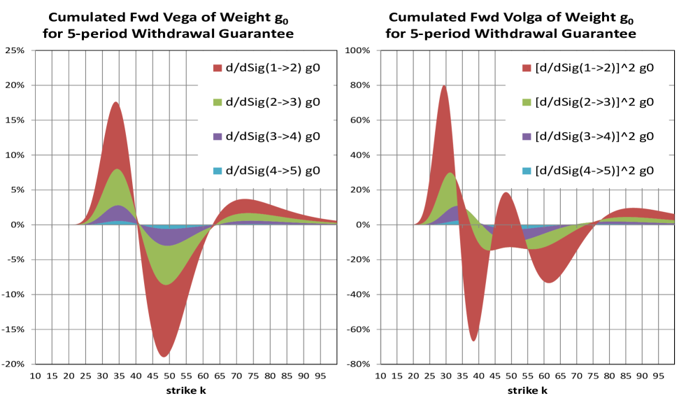
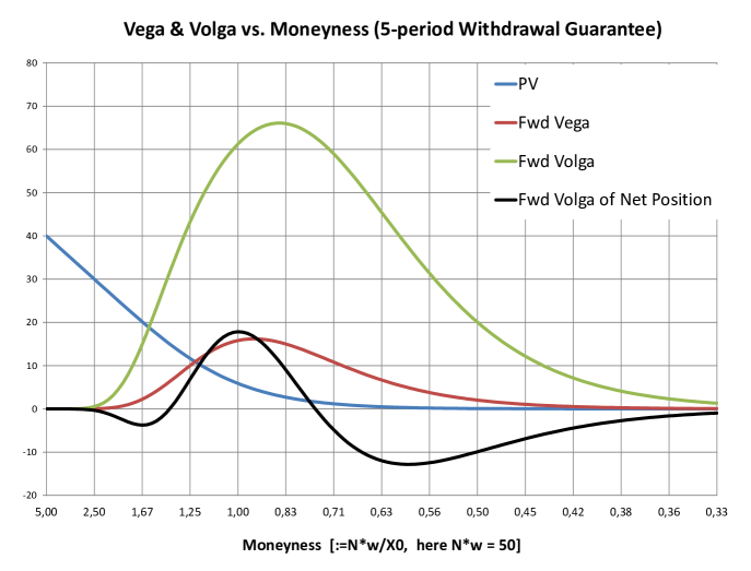
Figure 6: For a 5-period withdrawal guarantee, the top graph shows the forward vega and volga sensitivity of the weight function $g_{0}$, split into the sensitivity contributions with respect to the $T_{t}$-$T_{t+1}$-forward volatilities $\Sigma_{t}$ for $t=1,\dots,4$. The bottom graph displays present value and forward vega and volga sensitivities of the guarantee for different moneyness levels together with the volga of the net position after hedge with forward starting variance swaps. The results are very similar to those in the two-period case, see figure 3. Setting: Black-Scholes model as in two-period case.

1. The effects of stochastic volatility are very similar to the two-period case. Figure 6 displays for the 5-period case the total forward vega and volga sensitivity of the weight function $g_{0}$ and the split into the sensitivities with respect to the series of yearly forward volatilities. Similar to the two-period case, there is a net volga long position (after hedging with forward starting variance swaps) except for very in- and out-of-the-money guarantees. Hence, stochastic volatility models will price the guarantee at lower values than the corresponding local volatility model.

   [Figure 6 should be inserted here]

2. For one-factor exponential Lévy models, the semi-static hedging representation (30) allows a very efficient calculation of the withdrawal guarantee value and its sensitivities with respect to changes in the fund value and in the short-term volatility of the underlying. This is essential for the risk management of such products.

3. For non-zero deterministic interest rates, the static hedging representations (4) and (22) remain valid, since the discounting effects are already correctly reflected in the put option values and their derivatives.

   Due to the long-term nature of typical GMWB products, stochastic interest rates seem an indispensable ingredient for the valuation model at first glance. Unfortunately, our approach has no straightforward generalization to stochastic interest rates. Table 1 summarizes the interest rate volatility sensitivity for at-the-money GMWB products valuated in the one-factor Hull-White & Black-Scholes hybrid model (using Monte-Carlo techniques) and compares it to the sensitivities of vanilla put options und puts on multi-contribution funds: interest rate volatility sensitivity for withdrawal guarantees increases with maturity to ca. 1.5% of the base guarantee value for maturities of 30 years but remains at only ca. 30-35% of that of the corresponding vanilla put with same notional. Things are different for puts on multi-contribution funds which show much higher interest rate volatility sensitivity. The reason is that the withdrawals diminish the fund value and hence the volatility exposure relatively quickly in average whereas the multi-contribution fund accumulates the volatility exposure over run time.

   [Table 1 should be inserted here]

   This analysis shows that the need for stochastic interest rates for the valuation model of GMWB products is less pronounced compared to long-term vanilla options and puts on multi-contribution funds.

4. The presented semi-static hedging results do not only apply to simple withdrawal guarantee structures introduced in section 2. They immediately extend to non-constant deterministic schedules of withdrawal amounts. The technique also extends to roll-up or ratchet features, that are very common for GMWB products, see (4).

Appendix A Appendix: Proofs

Proof of (13). For the function $S_{1}\mapsto V_{1}(S_{1})$ that is piecewise defined in (11), we show that $V_{1}$ and $V_{1}^{\prime}$ is continuous at $S_{1}=w/\zeta_{0}$ and that $V_{1}^{\prime}=o(1/S_{1})$ as $S_{1}\nearrow\infty$. The second boundary condition $V_{1}(0)=2w$ is obvious.

First note that $V_{1}^{\prime}=[\partial_{S_{1}}+(\partial_{S_{1}}\zeta_{1})\cdot\partial_{\zeta_{1}}]\cdot[\zeta_{1}\cdot P_{1}\left(w/\zeta_{1}\right)]$ for $S_{1}>w/\zeta_{0}$ and hence

$$V_{1}^{\prime} = \zeta_{1}\cdot\Delta_{1}\left(\frac{w}{\zeta_{1}}\,\Big{|}\,S_{1}\right)+\frac{w}{S_{1}^{2}}\cdot\left[P_{1}\left(\frac{w}{\zeta_{1}}\,\Big{|}\,S_{1}\right)-\partial_{\mathcal{K}}P_{1}\left(\frac{w}{\zeta_{1}}\,\Big{|}\,S_{1}\right)\cdot\frac{w}{\zeta_{1}}\right]\,.$$ (37)

From the definition of $V_{1}$ in (11), we obtain $\lim_{S_{1}\nearrow w/\zeta_{0}}V_{1}(S_{1})=w$ and $\lim_{S_{1}\nearrow w/\zeta_{0}}V_{1}^{\prime}(S_{1})=-\zeta_{0}$. Further, $S_{1}\searrow w/\zeta_{0}$ implies $\zeta_{1}\searrow 0$. Hence,

$$\lim_{S_{1}\searrow w/\zeta_{0}}V_{1}(S_{1})=\lim_{\zeta_{1}\searrow 0}\zeta_{1}P_{1}\left(w/\zeta_{1}\right)=\lim_{\zeta_{1}\searrow 0}{\mathbb{E}}^{\mathbb{Q}}_{1}(w-\zeta_{1}S_{2})^{+}=w\,,$$

where the last equality follows from monotone convergence. Similarly, we obtain using (37)

$$\lim_{S_{1}\searrow w/\zeta_{0}}V_{1}^{\prime}(S_{1}) = \lim_{\zeta_{1}\searrow 0}\zeta_{1}\cdot\Delta_{1}\left(\frac{w}{\zeta_{1}}\,\Big{|}\,\frac{w}{\zeta_{0}}\right)+\frac{\zeta_{0}^{2}}{w}\cdot\lim_{\zeta_{1}\searrow 0}\left[P_{1}\left(\frac{w}{\zeta_{1}}\,\Big{|}\,\frac{w}{\zeta_{0}}\right)-\frac{w}{\zeta_{1}}\cdot\partial_{\mathcal{K}}P_{1}\left(\frac{w}{\zeta_{1}}\,\Big{|}\,\frac{w}{\zeta_{0}}\right)\right]$$

$$= \frac{\zeta_{0}^{2}}{w}\cdot\lim_{\zeta_{1}\searrow 0}{\mathbb{E}}^{\mathbb{Q}}_{1}\left[\left(\frac{w}{\zeta_{1}}-S_{2}\right)\cdot{\rm\bf 1}_{{w}/{\zeta_{1}}>S_{2}}-\frac{w}{\zeta_{1}}\cdot{\rm\bf 1}_{{w}/{\zeta_{1}}>S_{2}}\,\Big{|}\,S_{1}=\frac{w}{\zeta_{0}}\right]$$

$$= \frac{\zeta_{0}^{2}}{w}\cdot\lim_{\zeta_{1}\searrow 0}{\mathbb{E}}^{\mathbb{Q}}_{1}\left[-S_{2}\cdot{\rm\bf 1}_{{w}/{\zeta_{1}}>S_{2}}\,\Big{|}\,S_{1}=\frac{w}{\zeta_{0}}\right]$$

$$= \frac{\zeta_{0}^{2}}{w}\cdot{\mathbb{E}}^{\mathbb{Q}}_{1}\left[-S_{2}\,\Big{|}\,S_{1}=\frac{w}{\zeta_{0}}\right]=\frac{\zeta_{0}^{2}}{w}\cdot\left[-\frac{w}{\zeta_{0}}\right]=-\zeta_{0}\,,$$

where the second line uses the fact that $\Delta_{1}$ is bounded and the first equality in the last line above follows again from monotone convergence. This proves the continuity of $V_{1}$ and $V_{1}^{\prime}$ at $S_{1}=w/\zeta_{0}$.

Finally, $S_{1}\nearrow\infty$ implies $\zeta_{1}\to\zeta_{0}$. Hence we obtain using (37)

$$\lim_{S_{1}\nearrow\infty}S_{1}\cdot V_{1}^{\prime}(S_{1}) = \frac{w}{S_{1}}\cdot\left[P_{1}\left(\frac{w}{\zeta_{0}}\,\Big{|}\,S_{1}\right)-\partial_{\mathcal{K}}P_{1}\left(\frac{w}{\zeta_{0}}\,\Big{|}\,S_{1}\right)\cdot\frac{w}{\zeta_{0}}\right]=0\,,$$

since all terms in $[\cdot]$-brackets are bounded functions of $S_{1}$. Hence, $V_{1}^{\prime}=o(1/S_{1})$ as $S_{1}\nearrow\infty$. ∎

The following lemmata deal with implications of the assumption (A2).

Lemma 2.

(A2) is equivalent to assume that $S$ has independent returns, i.e. $S_{t+1}/S_{t}$ is independent on $S_{t}$ for every $t=1,\dots,N$.

Proof.

$\Leftarrow$ is obvious. To show $\Rightarrow$, note that by static hedging theory
${\mathbb{Q}}(S_{t+1}/S_{t}\leq K\,|\,S_{t}=s)={\mathbb{Q}}(S_{t+1}\leq s\cdot K\,|\,S_{t}=s)=\partial_{\mathcal{K}}P_{t}(s\cdot K\,|\,s)$.
It suffices to proof that $\partial_{\mathcal{K}}P_{t}(s\cdot K\,|\,s)$ is independent of $s$ for every $K>0$:
(A2) implies $P_{t}(k\,|\,s^{\prime})=k\cdot P_{t}(1\,|\,s^{\prime}/k)$. Hence $\partial_{k}P_{t}(k\,|\,s^{\prime})=P_{t}(1\,|\,s^{\prime}/k)-(s^{\prime}/k)\cdot\Delta_{t}(1\,|\,s^{\prime}/k)$. Thus $\partial_{\mathcal{K}}P_{t}(s\cdot K\,|\,s)=P_{t}(1\,|\,1/K)-(1/K)\cdot\Delta_{t}(1\,|\,1/K)=\partial_{\mathcal{K}}P_{t}(K\,|\,1)$.∎

Lemma 3.

(A2) implies that $x\cdot\Delta_{t}(k\,|\,x)\to 0$ and $k\cdot\partial_{\mathcal{K}}C_{t}(k\,|\,x)\to 0$ as $x,k\nearrow\infty$ uniformly in $k\in{\mathbb{R}}$ and $x\in{\mathbb{R}}$ for every $t=0,\dots,N-1$.

Proof.

Assumption (A2) implies $P_{t}(k\,|\,x)=x\cdot P_{t}(k/x\,|\,1)$. Hence

$$x\cdot\Delta_{t}(k\,|\,x) = x\cdot D_{x}[x\cdot P_{t}(k/x\,|\,1)]=x\left[P_{t}(k/x\,|\,1)-x\cdot\partial_{\mathcal{K}}P_{t}(k/x\,|\,1)\cdot(k/x^{2})\right]$$ (38)

$$= P_{t}(k\,|\,x)-k\cdot{\mathbb{Q}}(S_{t+1}\leq k/x\,|S_{t}=1)\,,$$

where the last equation follows from (A2) and the Breeden-Litzenberger formula (12). As $x\nearrow\infty$, both terms converge to zero locally uniformly in $k$. The proof for $k\cdot\partial_{\mathcal{K}}C_{t}(k\,|\,x)$ follows from analog considerations.∎

Lemma 4.

If a twice differentiable function $f=f(x,y)$ satisfies $f(\alpha x,\alpha y)=\alpha f(x,y)$ for every $\alpha\in{\mathbb{R}}$, then $\partial_{\mathcal{X}}^{n}f(\alpha x,\alpha y)=\alpha^{1-n}\partial_{\mathcal{X}}^{n}f(x,y)$ and $\partial_{\mathcal{Y}}^{n}f(\alpha x,\alpha y)=\alpha^{1-n}\partial_{\mathcal{Y}}^{n}f(x,y)$ for $n\in{\mathbb{N}}$.

Proof.

Follows from $\alpha\partial_{x}^{n}f(x,y)=\partial_{x}^{n}(\alpha f(x,y))=\partial_{x}^{n}f(\alpha x,\alpha y)=\alpha^{n}\partial_{\mathcal{X}}^{l}f(\alpha x,\alpha y)$.

Proof of (24). Applying partial integration to (23) yields

$$V_{t-} \stackrel{{\scriptstyle(\ref{eqn:def_tilde_gt})}}{{=}} \int_{\max(w,\zeta_{t-1}S_{t})}^{\infty}(k-\zeta_{t-1}S_{t})\cdot\left(\int_{w}^{\infty}\Gamma_{t}(k^{\prime}\,|\,k-w)\,{g}_{t}(k^{\prime})\,dk^{\prime}\right)dk$$

$$= \left[(k-\zeta_{t-1}S_{t})\int_{w}^{\infty}\Delta_{t}(k^{\prime}\,|\,k-w)\,{g}_{t}(k^{\prime})\,dk^{\prime}\right]_{k=\max(w,\zeta_{t-1}S_{t})}^{\infty}$$

$$+\left\{-\int_{\max(w,\zeta_{t-1}S_{t})}^{\infty}\int_{w}^{\infty}\Delta_{t}(k^{\prime}\,|\,k-w)\,{g}_{t}(k^{\prime})\,dk^{\prime}\,dk\right\}\,.$$

We first analyze the term in $[\cdot]$-brackets. The upper bound contribution for the limit $k\nearrow\infty$ vanishes due to lemma 3. Hence the $[\cdot]$-term has only contributions from the lower bound, which reads

$$[\cdot] = -{\rm\bf 1}_{\zeta_{t-1}S_{t}<w}\cdot(w-\zeta_{t-1}S_{t})\int_{w}^{\infty}(-1)\cdot{g}_{t}(k^{\prime})\,dk^{\prime}$$

$$\stackrel{{\scriptstyle{(\ref{eqn:mean_weight_Gt})}}}{{=}} -X_{t}\cdot{\rm\bf 1}_{X_{t}<0}=X_{t}^{-}=Z^{(t)}\,.$$

When integrating the $\{\cdot\}$-term, we obtain

$$\{\cdot\} = -\left[\int_{w}^{\infty}P_{t}(k^{\prime}\,|\,k-w)\,{g}_{t}(k^{\prime})\,dk^{\prime}\right]_{k=\max(w,\zeta_{t-1}S_{t})}^{\infty}$$

$$= \int_{w}^{\infty}P_{t}\left(k^{\prime}\,\Big{|}\,\max(0,\zeta_{t-1}S_{t}-w)\right)\,{g}_{t}(k^{\prime})\,dk^{\prime}$$

$$= {\rm\bf 1}_{X_{t}\leq 0}\int_{w}^{\infty}k^{\prime}\,{g}_{t}(k^{\prime})\,dk^{\prime}+{\rm\bf 1}_{X_{t}>0}\int_{w}^{\infty}p_{t}(X_{t},k^{\prime})\,{g}_{t}(k^{\prime})\,dk^{\prime}$$

$$\stackrel{{\scriptstyle{(\ref{eqn:mean_weight_Gt})}}}{{=}} {\rm\bf 1}_{\tau=t}\cdot m_{t}+{\rm\bf 1}_{\tau>t}V_{t}\,.$$

Hence $V_{t-}=Z^{(t)}+{\rm\bf 1}_{\tau=t}\cdot m_{t}+{\rm\bf 1}_{\tau>t}V_{t}\stackrel{{\scriptstyle{(\ref{eqn:MuliPeriod_Tilde_Vt})}}}{{=}}{V}_{t}$, which proves (24). ∎

Proof of Lemma 1. For $l=0,1$, we deduce

$$\int_{0}^{\infty}s^{l}\cdot\Gamma(K|s)ds = \lim_{s^{*}\uparrow\infty}\{s^{l}\Delta(K|s)]_{s=0}^{s^{*}}-l\cdot[P(K,s)]_{s=0}^{s^{*}}\}={\rm\bf 1}_{l=0}+K\cdot{\rm\bf 1}_{l=1}\,,$$ (39)

since $\lim_{s^{*}\uparrow\infty}s^{*}\Delta(K|s^{*})=0$ in case $l=1$ by lemma 3.

(a): the density $\Gamma(k^{\prime}|k)dk$ integrates to one on $k\in[0,\infty)$ by (39). Chapman-Kolmogorov (CK) property for $\tilde{S}$ follows from the CK property of the put option value process $t\mapsto P_{t,N}(K|S_{t})={\mathbb{E}}_{t}[(K-S_{N})^{+}|S_{t}]$ (a martingale!) and twice differentiation with respect to $S_{t}$. (b): on a discrete time grid, (27) generates a Markov chain on ${\mathbb{R}}^{+}$. By halving successively the grid size, a consistent sequence of Markov chains is generated due to the CK property. This sequence of Markov chains can shown to be tight which guarantees the existence of a time-continuous limit process $\tilde{S}$. (c): ${\mathbb{E}}_{t}[\tilde{S}_{t^{\prime}}|\tilde{S}_{t}=k]=\int_{0}^{\infty}k^{\prime}\Gamma_{N-t^{\prime},N-t}(k|k^{\prime})dk^{\prime}=k$ by (39). The proof of (d) is analog to the proof of Lemma 2 with $\partial_{\mathcal{K}}P_{t}$ replaced by $\Delta_{t}$. To show the relation (28) for the log-return density of the ajoint process we assume without loss of generality that $\tilde{S}_{t}=1$. Hence

$$\tilde{{\mathbb{Q}}}\left(\ln\tilde{S}_{t^{\prime}}\leq\xi\,|\,\tilde{S}_{t}=1\right)=\tilde{{\mathbb{Q}}}\left(\tilde{S}_{t^{\prime}}\leq e^{\xi}\,|\,\tilde{S}_{t}=1\right)\;\stackrel{{\scriptstyle\eqref{eqn:DefRevAdjointGammaProc}}}{{=}}\;\int_{0}^{e^{\xi}}\Gamma_{N-t^{\prime},N-t}(1|k^{\prime})\,dk^{\prime}$$

$$=\Delta^{C}_{N-t^{\prime},N-t}(1\,|\,e^{\xi})\;\stackrel{{\scriptstyle L\ref{lemma:ScalingProp_Derivaties}}}{{=}}\;\Delta^{C}_{N-t^{\prime},N-t}(e^{-\xi}\,|\,1)$$

$$=C_{N-t^{\prime},N-t}(e^{-\xi}\,|\,1)+e^{-\xi}\cdot{\mathbb{Q}}(S_{N-t}>e^{-\xi}\,|\,S_{N-t^{\prime}}=1)$$

$$=\int_{e^{-\xi}}^{\infty}s\cdot{\mathbb{Q}}(S_{N-t}\in s+ds\,|\,S_{N-t^{\prime}}=1)=\int_{e^{-\xi}}^{\infty}s\cdot\mbox{$\frac{1}{s}$}\cdot{\mathbb{Q}}(\ln S_{N-t}\in\ln s+ds\,|\,S_{N-t^{\prime}}=1)\,,$$

where the second last equation follows analogously to relation (38). Differentiation with resprect to $\xi$ proves relation (28). (e): It sufficies to show

$${\mathbb{Q}}(S_{t^{\prime}}\in dk^{\prime}\,|\,S_{t}=k)=\Gamma_{t,t^{\prime}}(k\,|\,S_{t}=k)\,dk\qquad(t<t^{\prime}\in\{0,\dots,N\},\;k,k^{\prime}>0)\,.$$ (40)

Put-Call-Symmetry implies (see e.g. [3]) $C_{t}(K|S_{t})/\sqrt{K}=P_{t}(K^{\prime}|S_{t})/\sqrt{K^{\prime}}$ for any pair of strikes $K,K^{\prime}\geq 0$ with $K\cdot K^{\prime}=S_{t}^{2}$. Chose $K^{\prime}=S_{t}^{2}/K$. Multiplying by $\sqrt{K}$ and applying call-put-parity gives $P_{t}(K|S_{t})+S_{t}-K=C_{t}(K|S_{t})=\sqrt{K}\cdot(\sqrt{K}/{S_{t}})\cdot P_{t}\left({S_{t}^{2}}/{K}\,|S_{t}\right)\stackrel{{\scriptstyle(A2)}}{{=}}P_{t}\left(S_{t}|K\right)\,.$ Differentiating twice with respect to $S_{t}$ and setting $K=k^{\prime}$ and $S_{t}=k$ yields $\Gamma_{t}(k^{\prime}\,|\,k)=\partial_{\mathcal{K}}^{2}P_{t}(k\,|\,k^{\prime})$ and (40) follows from the classical static hedging relation $\partial_{\mathcal{K}}^{2}P(k|k^{\prime})={\mathbb{Q}}(S_{t+1}\in dk\,|\,S_{t}=k^{\prime})$. ∎

Proof of (4). We apply static hedging techniques to the conditional expectation $\bar{V}^{R}_{t}$ in (33). (A2) implies that the density of $X_{t+1}+w_{t}=X_{t}\cdot(S_{t+1}/S_{t})$ is given by

$${\mathbb{Q}}(X_{t+1}+w_{t}\in dk)=\partial_{\mathcal{K}}^{2}P_{t}(k|X_{t})\,dk=\partial_{\mathcal{K}}^{2}C_{t}(k|X_{t})\,dk\,.$$

Since $V^{R}_{t+1}=V^{R}_{t+1}(w_{t},X_{t+1})$ defined in (4) is continuous in $X_{t+1}$ and $\partial_{X_{t+1}}V^{R}_{t+1}$ except at the roll-up point $X_{t+1-}+w_{t}=X_{t+1}={A}_{t+1}w_{t}$, we obtain by splitting the integration at $X_{t+1-}=(1+{A}_{t+1})w_{t}$

$$\bar{V}^{R}_{t}(w_{t},X_{t}) = \left[\int_{0}^{w_{t}(1+{A}_{t+1})}\partial_{\mathcal{K}}^{2}P_{t}(k|X_{t})+\int_{w_{t}(1+{A}_{t+1})}^{\infty}\partial_{\mathcal{K}}^{2}C_{t}(k|X_{t})\right]V_{t+1}^{R}(w_{t},k-w_{t})\,dk$$

$$= \Big{[}\partial_{\mathcal{K}}P_{t}(k|X_{t})\cdot V_{t+1}^{R}(w_{t},k-w_{t})\Big{]}_{k=0}^{w_{t}(1+{A}_{t+1})}$$

$$+\Big{[}\partial_{\mathcal{K}}C_{t}(k|X_{t})\cdot V_{t+1}^{R}(w_{t},k-w_{t})\Big{]}_{k=w_{t}(1+{A}_{t+1})}^{\infty}$$

$$-\Big{[}P_{t}(k|X_{t})\cdot\partial_{X_{t+1}}V_{t+1}^{R}(w_{t},k-w_{t}-0)\Big{]}_{k=0}^{w_{t}(1+{A}_{t+1})}$$

$$-\Big{[}C_{t}(k|X_{t})\cdot\partial_{X_{t+1}}V_{t+1}^{R}(w_{t},k-w_{t}+0)\Big{]}_{k=w_{t}(1+{A}_{t+1})}^{\infty}$$

$$+\left[\int_{0}^{w_{t}(1+{A}_{t+1})}P_{t}(k|X_{t})+\int_{w_{t}(1+{A}_{t+1})}^{\infty}C_{t}(k|X_{t})\right]\partial_{X_{t+1}}^{2}V_{t+1}^{R}(w_{t},k-w_{t})\,dk$$

$$= V_{t+1}^{R}(w_{t},w_{t}{A}_{t+1})$$

$$+\,C_{t}\left(w_{t}(1+{A}_{t+1})|X_{t}\right)\cdot\partial_{X_{t+1}}V_{t+1}^{R}(w_{t},w_{t}{A}_{t+1}+0)$$

$$-\,P_{t}\left(w_{t}(1+{A}_{t+1})|X_{t}\right)\cdot\partial_{X_{t+1}}V_{t+1}^{R}(w_{t},w_{t}{A}_{t+1}-0)$$

$$+\int_{1}^{1+{A}_{t+1}}P_{t}(w_{t}k|X_{t})\cdot\partial_{X_{t+1}}^{2}V_{t+1}^{R}(w_{t},w_{t}(k-1))\,w_{t}\,dk$$

$$+\int_{1+{A}_{t+1}}^{\infty}C_{t}(w_{t}k|X_{t})\cdot\partial_{X_{t+1}}^{2}V_{t+1}^{R}(w_{t},w_{t}(k-1))\,w_{t}\,dk\,,$$

where the last equality follows from the boundary conditions for $V_{t}$ (and hence also for $V^{R}_{t}$) at $X_{t}=0$ analog to (13), the relation $\partial_{\mathcal{K}}P_{t}(k)=\partial_{\mathcal{K}}C_{t}(k)+1$ stemming from put-call-parity, the fact that $\partial_{X_{t+1}}^{2}V_{t+1}^{R}(k-w_{t},w_{t})\equiv 0$ on $k\in[0,w_{t}]$, and the change of integration variable $k\mapsto k/w_{t}$, provided that

$$\lim_{k\nearrow\infty}\partial_{\mathcal{K}}C_{t}(k)\cdot V_{t+1}^{R}(w_{t},k-w_{t})=\lim_{k\nearrow\infty}C_{t}(k)\cdot\partial_{X_{t+1}}V_{t+1}^{R}(w_{t},k-w_{t})=0\,.$$ (41)

Now suppose that $\bar{V}^{R}_{t+1}$ satisfies (A2), i.e. $\bar{V}^{R}_{t+1}(\alpha\cdot w_{t+1},\alpha\cdot X_{t+1})=\alpha\cdot\bar{V}^{R}_{t+1}(w_{t+1},X_{t+1})$ for every $\alpha>0$.

For $X_{t+1}>w_{t}{A}_{t+1}$, we then obtain by (4) that $V_{t+1}^{R}(w_{t},X_{t+1})=\bar{V}_{t+1}^{R}(X_{t+1}/{A}_{t+1},X_{t+1})=X_{t+1}\cdot\bar{V}_{t+1}^{R}(1/{A}_{t+1},1)$. Hence $\partial_{X_{t+1}}V_{t+1}^{R}\equiv\bar{V}_{t+1}^{R}(1/{A}_{t+1},1)=\bar{V}_{t+1}^{R}(1,{A}_{t+1})/{A}_{t+1}$ and $\partial_{X_{t+1}}^{2}V_{t+1}^{R}\equiv 0$. In particular, assumption (41) is satisfied together with lemma 3. For any real number $x\leq{A}_{t+1}$, we deduce together with lemma 4 that $\partial_{X_{t+1}}^{l}V_{t+1}^{R}(w_{t},w_{t}x)=\partial_{X_{t+1}}^{l}\bar{V}_{t+1}^{R}(w_{t},w_{t}x)=$ $w_{t}^{1-l}\partial_{X_{t+1}}^{l}\bar{V}_{t+1}^{R}(1,x)$ for $l=1,2$.

Summarizing all effects of the assumption that $\bar{V}^{R}_{t+1}$ satisfies (A2) allows to rewrite

$$\bar{V}^{R}_{t}(w_{t},X_{t}) = w_{t}\cdot\bar{V}_{t+1}^{R}(1,{A}_{t+1})$$

$$+\,C_{t}\left(w_{t}(1+{A}_{t+1})|X_{t}\right)\cdot\bar{V}_{t+1}^{R}(1,{A}_{t+1})/{A}_{t+1}$$

$$-\,P_{t}\left(w_{t}(1+{A}_{t+1})|X_{t}\right)\cdot\partial_{X_{t+1}}\bar{V}_{t+1}^{R}(1,{A}_{t+1})$$

$$+\int_{1}^{1+{A}_{t+1}}P_{t}(w_{t}k|X_{t})\cdot w_{t}^{-1}\cdot\partial_{X_{t+1}}^{2}\bar{V}_{t+1}^{R}(1,k-1)\cdot w_{t}\,dk\,.$$

This representation shows that also $\bar{V}^{R}_{t}$ satisfies (A2), i.e. $\bar{V}^{R}_{t}(\alpha\cdot w_{t},\alpha\cdot X_{t})=\alpha\cdot\bar{V}^{R}_{t}(w_{t},X_{t})$ for every $\alpha>0$. Since the terminal term $\bar{V}^{R}_{N-1}=\bar{V}^{R}_{N-1}(w_{N-1},X_{N-1})=P_{N-1}(w_{N-1}|X_{N-1})$ clearly satisfies (A2) (as $S$ satisfies (A2) by assumption), backwards induction shows that $\bar{V}^{R}_{t}$ satisfies (A2) for every $t=0,\dots,N-1$.

Relation (A) delivers the identification (36) of the constants $\alpha_{t}$,$\beta_{t}$ and the weight functions $g^{R}_{t}$. Differentiation of the backward recursions (A) applied to $\bar{V}^{R}_{t+1}$ with respect to $X_{t+1}$ leads to the backwards recursions (4) for $\alpha_{t}$, $\beta_{t}$ and $g^{R}_{t}$. ∎

	NPV		Sensitivity
	base	HW vol	absolut	in % npv	in % sensi
		+0.1%		base	vanilla put
10y
vanilla put	8.108	8.153	0.045	0.55%
withdrawal guarantee	5.122	5.135	0.013	0.26%	30.07%
put on mlt-contrb. fund	4.754	4.783	0.028	0.60%	63.03%
20y
vanilla put	18.288	18.603	0.314	1.72%
withdrawal guarantee	11.989	12.090	0.101	0.84%	32.20%
put on mlt-contrb. fund	10.903	11.105	0.203	1.86%	64.46%
30y
vanilla put	27.809	28.605	0.796	2.86%
withdrawal guarantee	19.088	19.377	0.289	1.52%	36.32%
put on mlt-contrb. fund	16.900	17.437	0.537	3.18%	67.45%

Table 1: Interest rate volatility sensitivity comparison for the following products with maturities of 10, 20 and 30 years: (a) vanilla put, (b) withdrawal guarantee and (c) put on multi-contribution fund. The values are calculated under the hybrid one-factor Hull-White & Black-Scholes model (2% flat initial forward rate, 3% mean reversion and 1% volatility of short rate, 25% excess voatility of underlying with zero correlation to short rate). The regular withdrawals or contributions are assumed to occur quarterly with unit amount. The guarantees are assumed at-the-money such that the initial fund value or the strikes are set equal to the sum of the regular withdrawals or contributions, respectively. The vanilla put is valuated analytically, the other guarantees are priced with a Monte-Carlo approach (using $10^{5}$ scenarios).

Figure 1: These graphics illustrate the contingent withdrawal guarantee payments. The guarantor has to finance the outstanding withdrawal payments in case the fund is depleted before maturity. The smaller red arrow corresponds to the expression $X_{t}^{-}$ in the representation of the contingent withdrawal guarantee payment $Z^{(t)}$ due at withdrawal time $T_{t}$.

Figure 5: This graphic displays the densities of the weight functions ${g}_{t}$ defined in (21), with $t$ stepping backwards from $N-1$. The terminal weight function ${g}_{N-1}$ is given by Dirac’s point measure concentrated at the withdrawal amount $w=10$. Recall that $g_{t}(k)dk$ describes the weight of put options in the hedge portfolio at withdrawal time $T_{t}$ with strikes in a small range $dk$ around $k$. Setting: Black-Scholes model with volatility $=0.3$, zero interest rate and dividend yield.

Figure 7: Density of the log-return $\ln(S_{t}/S_{0})$ of the original process $S$ and the reverse $\Gamma$-adjoint process in the variance gamma model. The parameter are set to those reported in the seminal paper [5], Table II, on the variance gamma model. Interest rates are set to $2\%$ flat.

Figure 8: Net present value of withdrawal guarantees in variance gamma model for maturities of 10, 20 and 30 years and different moneyness levels: the blue values are obtained by sampling from the density of the reverse $\Gamma$-adjoint asset process and calculating the density of the associated multi-contribution fund according to (30). These results are compared with a straightforward Monte-Carlo valuation (red) that samples directly from the distribution of the underlying. The variance gamma model is calibrated as in figure 7, regular withdrawals are assumed to occur quarterly with unit amount and moneyness is defined as total sum of withdrawal amounts in percent of initial fund value. Monte-Carlo simulations are performed with $10^{5}$ scenarios.

References

- [1] Blamont, D. and Sagoo, P. (2009): Pricing and hedging of variable annuities, Life & Pensions RISK, February 2009.
- [2] Breeden, D.T. and Litzenberger, R.H. (1978): Prices of State-Contingent Claims Implicit in Option Prices Static Hedging, Journal of Business, 51/ 4, 621-51.
- [3] Carr, P., Ellis, K. and Gupta, V. (1998): Static Hedging of Exotic Options, Journal of Finance, June 1998, 1165-90.
- [4] Karatzas, I. and Shreve, S.E. (1998): Methods of Mathematical Finance, Springer 1998, New York.
- [5] Madan, D., Carr, P., and Chang, E. (1998): The variance gamma process and option pricing, European Finance Review, 2:79 -105.
- [6] Milevsky, M.A. and Salisbury, T.S. (2006): Financial valuation of guaranteed minimum withdrawal benefits, Insurance: Mathematics & Economics, 38/ 1, 21-38.
- [7] Tankov, P. (2010): Pricing and hedging in exponential Levy models: review of recent results, Paris-Princeton Lecture Notes in Mathematical Finance, Springer 2010.