$P$-values, $q$-values and posterior probabilities for equivalence in genomics studies

Abstract

Equivalence testing is of emerging importance in genomics studies but has hitherto been little studied in this content. In this paper, we define the notion of equivalence of gene expression and determine a ‘strength of evidence’ measure for gene equivalence. It is common practice in genome-wide studies to rank genes according to observed gene-specific $P$-values or adjusted $P$-values, which are assumed to measure the strength of evidence against the null hypothesis of no differential gene expression. We show here, both empirically and formally, that the equivalence $P$-value does not satisfy the basic consistency requirements for a valid strength of evidence measure for equivalence. This means that the widely-used $q$-value (Storey, 2002) defined for each gene to be the minimum positive false discovery rate that would result in the inclusion of the corresponding $P$-value in the discovery set, cannot be translated to the equivalence testing framework. However, when represented as a posterior probability, we find that the $q$-value does satisfy some basic consistency requirements needed to be a credible measure of evidence for equivalence. We propose a simple estimate for the $q$-value from posterior probabilities of equivalence, and analyse data from a mouse stem cell microarray experiment which demonstrate the theory and methods presented here.

Keywords: EM algorithm; equivalence testing; false discovery rate; $P$-value; posterior probability; $q$-value; stem cell microarray experiment.

1 Introduction

1.1 Motivation for equivalence testing in genomics

Equivalence testing is pervasive in the pharmaceutical industry for assessing whether two drugs or treatment regimens provide comparable therapeutic effects within pre-defined clinical and statistical limits (Senn, 2001; Chow and Liu, 2008). Typically, a new treatment formulation is of interest if it potentially provides an equivalent therapeutic effect with fewer adverse side-effects than the standard treatment, or is less costly to produce. In such trials, a fixed level of statistical significance is usually prescribed and within this context, tests based on confidence interval inclusion provide a sound basis for analysis (Westlake, 1972; Wellek, 2003).

Recently, a number of important applications entailing hypotheses of equivalence have arisen in the area of microarray bioinformatics and genomics studies, as illustrated by the following.

Illustration 1: Gene profiling. There are biological problems in which it is desired to establish that the levels of expression for certain genes remain constant across different conditions and/or points in time. Tuke et al. (2009) propose a general method for ranking genes according to their conformance to a pre-specified profile of expression over time, known as gene profiling. In many situations, the expected time-course profile dictates that gene expression should remain the same, or be equivalent, at two or more different time points, and hence equivalence testing methods are required as part of the statistical inferential framework.

Illustration 2: Experimental study of regulatory $T$ cells of the immune system. $CD4^{+}CD25^{+}$ regulatory $T$ cells (known as $CD4^{+}$ Treg cells) play a central role in the human immune system, including in the immunopathogenesis of autoimmune diseases, tumours, viral infections such as HIV, and organ transplants (Wei, 2006). Naturally occurring $CD4^{+}$ Treg cells are available only in very small quantities however, and for this reason many in vitro experiments are conducted on induced cell populations. To ensure the integrity of such experiments, it is desirable to establish that gene expression is equivalent between the naturally occurring and induced cells, at least under baseline conditions. The establishment of such conditions requires direct formal testing of an equivalence hypothesis, rather than simply failing to find evidence of differential expression between the two populations.

Illustration 3: Normalisation and quality assurance. A third and common problem for which methods of equivalence testing are appropriate in practice (although not always applied) is in the identification of highly stable genes or set of genes for the purpose of quality assurance, or for normalisation for use in future experiments. The identification of such genes (often housekeeping genes of some variety) is particularly important in large-scale studies utilising a reference population and conducted over time, such as in cancer studies. The reference population may be subject to temporal or other changes, and linkage experiments are usually conducted to ensure comparability of results and diagnoses over time.

In each of these illustrations, the aim of the scientific experiment is to test one or more hypotheses of equivalence. In a typical experiment, many thousands of genes will be tested simultaneously, and a primary goal of an initial bioinformatics exploratory analysis, known as a ‘gene-screen’, is to produce a ranked gene list. Therefore, we require an inferential strength of evidence measure for equivalence which will give just such a ranking.

Now, we know that there are two types of mistakes we can make when testing a statistical hypothesis: the first is Type I error, which is the probability of rejecting the null hypothesis when it is true, and the second is Type II error, which is the probability of retaining the null hypothesis when it is false. Type I errors are also known as false positives, and it is their dramatically increased frequency in genomics applications which has received most attention. A popular approach to adjusting for multiple hypotheses testing in this context is to find the observed $P$-value for each gene, and then to calculate its associated $q$-value (Storey, 2003). For each gene, the observed $q$-value is the positive false discovery rate (pFDR) that would result in the corresponding $P$-value being included in the discovery set, should this be the adjustment procedure applied. The pFDR itself is the rate at which genes are incorrectly discovered to be significant; there are also other methods for controlling the Type I error at a reasonable level, for example, controlling the overall family-wise error rate, but the pFDR is popularly applied in genomics studies.

In Section 2, we review the formal definition of the $q$-value, then derive the equivalence $P$-value for each gene. We show that our $P$-value equates to alternative derivations by Senn (2001) and Ge et al. (2003). We then point out problems with equivalence $P$-values, in particular, that they tend to zero as the standard error of the estimator increases, and that they are non-monotonic, thus rendering them unsuitable as a basis for calculating equivalence $q$-values. In Section 3, we describe the $q$-value as a posterior probability, and prove that the equivalence $q$-value obtained in this way is a monotonic function of the standard error of the estimator of interest, thus satisfying the basic consistency requirement (among other things) for a strength of evidence measure for the gene ranking. We also show how to estimate $q$-values from the observed posterior probabilities for equivalence.

In Section 4, we set out our motivating analysis of a murine stem cell microarray experiment conducted at the University of Adelaide. The overall aim of the larger time course experiment was to identify and investigate genes involved in pluripotency. We are interested in which of the $23,040$ mouse genes are equivalently expressed at day 0 (i.e., the beginning of the experiment) and at day 3. We begin by proposing a joint probability model for the observed and true log ratios to obtain the posterior probability of equivalence; we employ an empirical rather than a fully Bayesian approach to estimation, utilising the EM algorithm to estimate the specified hyperparameters. We finish with a brief conclusion in Section 5 extolling the virtues of the $q$-value, when represented as a posterior probability, as a credible measure of evidence for equivalence.

2 Equivalence $P$-values and $q$-values

2.1 The positive false discovery rate and the $q$-value

We are interested in the positive false discovery rate (pFDR) due to Storey (2003). To review, Table 1 gives the possible outcomes when $m$ hypotheses tests are performed according to some significance rule:

	Accept null	Reject null	Total
Null true	U	V	$m_{0}$
Alternative true	T	S	$m_{1}$
	W	R	m

Table 1: Possible outcomes from $m$ hypotheses tests.

The positive false discovery rate is then defined as

$$\text{pFDR}=E\left[V/R|R>0\right]$$

In genomics studies, and for equivalence testing in particular, $R>0$ almost always, so we assume from now on that the pFDR is the same as the FDR.

Now suppose that for each of the $m$ hypotheses, the test statistics
$T_{1},T_{2},\ldots,T_{m}$ are observed. Consider a nested set of significance regions denoted by $\Gamma_{\alpha},0\leq\alpha\leq 1$, where $\alpha$ is such that

$$P(T_{i}\in\Gamma_{\alpha}|i\text{th null hypothesis is true})=\alpha$$

and $\alpha^{\prime}\leq\alpha$ implies that $\Gamma_{\alpha^{\prime}}\subset\Gamma_{\alpha}$. Storey (2003) defines the $q$-value for an observed test statistic $T=t$ to be

$$q\text{-value}(t)=\inf_{\Gamma_{\alpha}:t\in\Gamma_{\alpha}}\text{pFDR}(\Gamma_{\alpha})$$ (1)

We return to the general definition (1) in Section 3.

2.2 $P$-values for equivalence testing

Consider a parameter of interest $\theta$ and its associated estimator, $\hat{\theta}$, such that

$$\hat{\theta}\sim N(\theta,SE(\hat{\theta})^{2}),$$

i.e., $\hat{\theta}$ is an unbiased estimator of $\theta$. For simplicity, but without loss of generality, we assume that the standard error of the estimator $\hat{\theta}$ is known.

In statistical equivalence testing, the null and alternative hypotheses are, respectively,

$$H_{0} :|\theta|\geq\varepsilon,\quad\varepsilon>0,$$ (2)

$$H_{A} :|\theta|<\varepsilon$$ (3)

Consider now the test statistic,

$$U(\hat{\theta})=\frac{\varepsilon-|\hat{\theta}|}{SE(\hat{\theta})}$$ (4)

The test statistic is chosen so that large values give evidence in favour of $H_{A}$. From (4), we can deduce that as the observed value of the estimator gets closer to zero from either direction, then the test statistic increases to a maximum at $\varepsilon/SE(\hat{\theta})$, while as the observed value of the estimator moves away from zero, the test statistic decreases.

The following theorem is from Casella (2002, p.397):

Theorem 1: Let $W(\boldsymbol{X})$ be a test statistic such that large values of $W$ give evidence that $H_{A}$ is true. For each sample point $\boldsymbol{x}$, define

$$p(\boldsymbol{x})=\sup_{\theta\in\Theta_{0}}P_{\theta}(W(\boldsymbol{X})\geq W(\boldsymbol{x})),$$

where $\Theta_{0}$ is a subset of the parameter space defined by the null hypothesis. Then, $p(\boldsymbol{X})$ is a valid $P$-value.

Applying Theorem 1 to the test statistic (4) yields the $P$-value

$$P_{U} =\sup_{\theta\in\Theta_{0}}P_{\theta}(U(\hat{\theta})\geq u(\hat{\theta}))$$ (5)

$$=\sup_{|\theta|\geq\varepsilon}P_{\theta}\left(\frac{-|\hat{\theta}|-\theta}{SE(\hat{\theta})}\leq Z\leq  \frac{|\hat{\theta}|-\theta}{SE(\hat{\theta})}\right),$$ (6)

where $\hat{\theta}$ is the observed estimate and $Z\sim N(0,1)$. It can be shown that $P_{U}$ is maximised at $\theta=\pm\varepsilon$, so that

$$P_{U}=P\left(\frac{-|\hat{\theta}|-\varepsilon}{SE(\hat{\theta})}\leq Z\leq  \frac{|\hat{\theta}|-\varepsilon}{SE(\hat{\theta})}\right)$$ (7)

An alternative derivation of $P_{U}$ uses a Neyman-Pearson-type test, as proposed by Senn (2001). He considers the statistical problem of equivalence testing for a parameter of interest $\theta$, with an estimator $\hat{\theta}$, such that

$$\hat{\theta}\sim N(\theta,SE(\hat{\theta})^{2})$$

Then for a pair of symmetric critical values for $\hat{\theta}$, $-c$ and $c$, the power function for a test based on $\hat{\theta}$ is

$$\Phi\left(\frac{c-\varepsilon}{SE(\hat{\theta})}\right)-\Phi\left(\frac{-c-\varepsilon}{SE(\hat{\theta})}\right)$$ (8)

To achieve a test of significance level $\alpha$, equation (8) is set equal to $\alpha$ and solved for $c$.

In other work, Ge et al. (2003) state that the $P$-value is the minimum Type 1 error over all possible rejection regions that contain the observed value of the test statistic. Again consider the observed estimate $\hat{\theta}$. The $P$-value associated with this observed estimate, which is denoted by $P_{alt}$ can therefore be derived from the power function (8):

$$P_{alt} =\min_{c:\hat{\theta}\in(-c,c)}\Phi\left(\frac{c-\varepsilon}{SE(\hat{\theta})}\right)-\Phi\left(\frac{-c-\varepsilon}{SE(\hat{\theta})}\right)$$

$$=\Phi\left(\frac{|\hat{\theta}|-\varepsilon}{SE(\hat{\theta})}\right)-\Phi\left(\frac{-|\hat{\theta}|-\varepsilon}{SE(\hat{\theta})}\right)$$

$$=P_{U}$$

which again recovers our estimate (6).

2.3 Inconsistency of equivalence $P$-values

The $P$-value is often interpreted as a strength of evidence measure for the alternative hypothesis. For example, Casella and Berger (2002) state that small values of the $P$-value give evidence that the alternative hypothesis is true (Definition 8.3.26, page 397). This is not true, however, for equivalence $P$-values, as we now demonstrate.

Consider Equation $(6)$ as a function of $SE(\hat{\theta})$, with $\hat{\theta}$ and $\varepsilon$ fixed. In general, as $SE(\hat{\theta})$ increases, then $P_{U}$ decreases to zero. This is illustrated in Figure 1 which plots $P_{U}$ versus $SE(\hat{\theta})$ for values of $\hat{\theta}$ of $0.5$, $1$, and $2$, and $\varepsilon=1$. For each value of $\hat{\theta}$, as $SE(\hat{\theta})$ increases, then $P_{U}$ decreases to zero. Thus, small values of $P_{U}$ do not necessarily indicate evidence that the alternative hypothesis is true, i.e., that $\theta$ is equivalent to zero. For example, consider an observed value of $\hat{\theta}=0.5$, with $SE(\hat{\theta})=10$. For these observed values, we are $95$% confident that the true value of $\theta$ lies between $-19.09964$ and $20.09964$, but the observed value of $P_{U}$ for the equivalence margin of $(-1,1)$ is $0.03969$. This small value of $P_{U}$ indicates strong evidence that $\theta$ lies between $-1$ and $1$, which is false. In fact, the largest confidence interval that would be wholly contained within the equivalence margin is a $52$% confidence interval.

A further observation of note is the lack of monotonicity of $P_{U}$ as $SE(\hat{\theta})$ increases. This is illustrated by the graph of $P_{U}$ versus $SE(\hat{\theta})$ for the case $\hat{\theta}=0.5$ in Figure 1. As $SE(\hat{\theta})$ increases from $0$ to $1$, $P_{U}$ increases to a maximum of about $0.24$, then $P_{U}$ decreases as $SE(\hat{\theta})$ increases from $1$ to $20$. As a result of this lack of monotonicity, it is possible to have the same value of $P_{U}$ for different values of $SE(\hat{\theta})$. For example, the $P_{U}$ for an observed value of $\hat{\theta}=0.5$, an equivalence margin of $\varepsilon$ equal to $1$, and $SE(\hat{\theta})=0.3$, is $0.04779$. This is the same $P$-value that is observed for the same conditions but with $SE(\hat{\theta})$ equal to $8.28224$. To assign the same strength of evidence to both of these cases is incorrect.

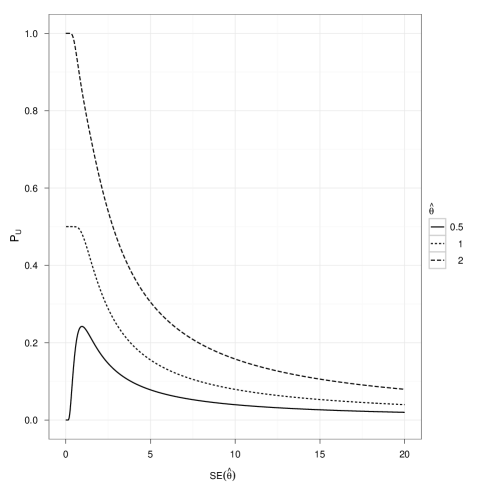
Figure 1: Equivalence $P$-value versus $SE(\hat{\theta})$ for an equivalence margin of $\varepsilon=1$.

These inconsistencies in interpretation of the observed equivalence $P$-values highlight the fact that they lack the basic consistency requirements necessary to provide a valid strength of evidence measure for equivalence, either on their own as raw (unadjusted) $P$-values, or as a basis for (adjusted) statistics such as the $q$-value.

We turn instead to a Bayesian formulation, and in particular, propose the posterior probability of equivalence, as an alternative strength of evidence measure for equivalence. We justify this approach in the next section and also show how to calculate approximate $q$-values from the posterior probabilities.

3 Monotonicity of posterior probabilities for equivalence and $q$-values

In Section 2.1, we defined the $q$-value, $q(t)$, for $m$ identical hypothesis tests with corresponding test statistics $T_{1},\dots,T_{m}$ and significance region $\Gamma$ (Storey, 2003).

For each hypothesis test, there is also a corresponding Bernoulli random variable $H_{i}$ with $H_{i}=0$ if the null hypothesis is true and $H_{i}=1$ if the null hypothesis is false. Storey (2003) assumes that $(T_{i},H_{i})$ are independent identically distributed random variables, $T_{i}|H_{i}\sim(1-H_{i})F_{0}+H_{i}F_{1}$ for some null distribution $F_{0}$ and alternative distribution $F_{1}$, and $H_{i}\sim$Bernoulli$(\pi)$ for $i=1,\ldots,m$, where $\pi$ is the a priori probability that a null hypothesis is false, i.e., $P(H_{i}=1)=\pi$. Therefore, the $q$-value is the infimum of the quantity $P(H=0|T\in\Gamma_{\alpha})$, that is, the posterior probability that the null hypothesis is true given that the test statistic is contained in the significance region of level $\alpha$.

The following theorem states that for equivalence testing, the $q$-value is monotonically decreasing for increasing variance of the test statistic. We state the theorem here and defer its proof to Appendix 2, which also contains the statement and proof of a lemma which is used in the proof of Theorem 2.

Theorem 2: Suppose $\theta$ has prior distribution $P(\theta)$ and $T|\theta\sim N(\theta,\sigma^{2})$. Consider numbers $0<\ell<\varepsilon$ and assume further that $0<P(-\varepsilon<\theta<\varepsilon)<1$. Then $P(-\varepsilon<\theta<\varepsilon\mid-\ell<T<\ell)$ is a decreasing function of $\sigma^{2}$.

Note that for given $SE({\hat{\theta}})$, the $q$-value is intended to estimate the posterior probability

$$1-P(-\varepsilon<\theta<\varepsilon\mid-\ell<T<\ell),$$

which we have therefore established increases monotonically with $SE({\hat{\theta}})$.

3.1 Estimating $q$-values from posterior probabilities of equivalence

Before illustrating the methods on the stem cell microarray data, we take the development a step further and show how to estimate $q$-values from the observed posterior probabilities of equivalence in any given application.

Consider an arbitrary cutoff point $t$ such that all genes will be considered equivalent if their observed posterior probability of equivalence is greater than or equal to $t$. The FDR for the cutoff $t$ is then

$$\text{FDR}(t)=E\left[\frac{V(t)}{R(t)}\right],$$

where $R(t)$ is the number of genes considered equivalent with assumed cutoff $t$, and $V(t)$ is the number of genes considered equivalent with cutoff $t$ that are not in fact equivalent, i.e., these are false positives. Storey (2003) recovers the general result that

$$E\left[\frac{V(t)}{R(t)}\right]\approx\frac{E[V(t)]}{E[R(t)]}$$

In the case of gene equivalence studies, $E[R(t)]$ can be estimated by the number of genes whose posterior probability of equivalence is greater than or equal to $t$. The estimate of $E[V(t)]$ is obtained by considering each hypothesis test as a Bernoulli random variable $X_{i},i=1,\ldots,m$, where $X_{i}=1$ if the null hypothesis is true, that is, $|\theta_{i}|\geq\varepsilon$, and $X_{i}=0$ if the null hypothesis is false. Therefore,

$$E[V(t)]=E\left[\sum_{i:p_{i}\geq t}X_{i}\right]=\sum_{i:p_{i}\geq t}E[X_{i}]=\sum_{i:p_{i}\geq t}q_{i},$$

where

$$q_{i}=P(|\theta_{i}|\geq\varepsilon),$$

and $p_{i}$ is the posterior probability of equivalence for the $i^{th}$ gene.

The value of $q_{i}$ is unknown but can be estimated from the posterior distribution of $\theta_{i}$ by $q_{i}\approx 1-p_{i}$, where $p_{i}$ is the posterior probability of equivalence of the $i$th gene. The estimated $q$-value for a cutoff point $t$ is then

$$\hat{q}(t) =\frac{\sum_{i:p_{i}\geq t}(1-p_{i})}{\#\{i:p_{i}\geq t\}},$$ (9)

where $\#A$ represents the cardinality of the set $A$.

In the next section we explore the performance of the posterior probabilities of equivalence for the stem cell data. We also estimate the approximate $q$-values obtained from the posterior probabilities of gene expression equivalence.

4 Gene equivalence in mouse stem cells on day 0 and day 3

Much of our work on gene equivalence has been motivated by a stem cell microarray experiment conducted at the University of Adelaide. The overall aim of the experiment was to identify and investigate genes involved in the cellular process of pluripotency; the details of this study and its design are described in Tuke et al. (2009) and Tuke (2012). Here we are interested in which of $23,040$ mouse genes are equivalently expressed at day 0 (i.e., the beginning of the experiment) and at day 3. This equivalence gene-set will include genes which are not expressed on either day and genes which are expressed on both day 0 and day 3. We know a priori that there are housekeeping genes included on the microarray which are highly and constantly expressed across hybridisations, and that there are genes involved in pluripotency which are also expressed on both days. There are two (dye-swapped) two-colour mouse Compugen long-oligonucleotide microarrays available for analysis, which are treated as independent replicates.

We proceed as follows: to begin, we specify a joint distribution for the true mean log ratio and the observed mean log ratio for each gene, in which the prior distribution for the true mean log ratio is a mixture model of three normal distributions. The hyperparameters for the joint distribution are then estimated from the observed mean log ratios using the EM algorithm (as described in Appendix 1) and finally the posterior distribution of the true gene log ratio is derived and used to calculate the posterior probability of equivalence. We do not use a fully Bayesian formulation for our case study, but rather estimate the hyperparameters then treat them as ‘known’, thereby utilising a simpler empirical Bayesian approach.

4.1 The probability model for each gene

The parameter of interest is the true mean log ratio which will be equal to zero if the gene is equivalently expressed on day 3 and day 0.

If the true mean log ratio for gene $i$ is denoted by ${\theta_{i}}$, $i=1,...,23040$, then the sample mean of the observed log ratio, $Y_{i}$, is assumed to be normally distributed with mean $\theta_{i}$ and variance $\sigma^{2}_{i}$, which is assumed known. The probability density function for $Y_{i}$ is then

$$f(y_{i}|\theta_{i})=\frac{1}{\sqrt{2\pi\sigma_{i}^{2}}}\exp\left[-\frac{(y_{i}-\theta_{i})^{2}}{2\sigma_{i}^{2}}\right]$$

The prior probability distribution for $\theta_{i}$ is assumed to be a mixture model of three normal distributions. This choice of prior gives flexibility to the full probability model and is motivated by the data. Figure 2 presents a histogram of the observed mean log ratios for day 3 compared to day 0 for the data $y_{i}$, and shows a symmetric bell-shaped density with relatively heavy tails compared to a normal density. This suggests a $t$-distribution with a small number of degrees of freedom would be an appropriate prior, among other possibilities, and it is straightforward to show that such a $t$-distribution is well approximated by a mixture of three normal distributions.

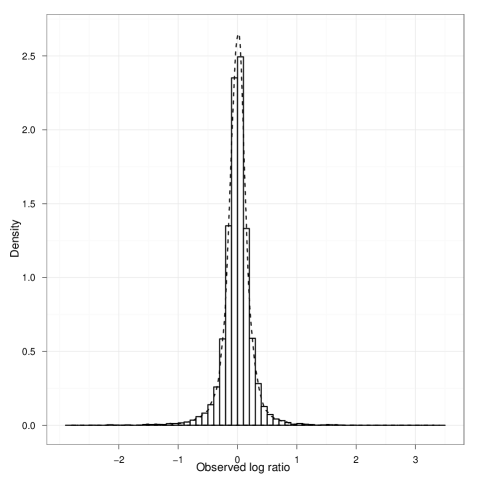
Figure 2: Histogram of observed mean log ratios for day 3 compared to day 0 for the mouse stem cell data.

The prior distribution for $\theta_{i},i=1,\ldots,23040$ is therefore

$$f(\theta_{i})=\sum^{3}_{j=1}\frac{\pi_{j}}{\sqrt{2\pi\tau^{2}_{j}}}\exp\left[-\frac{(\theta_{i}-\mu_{j})^{2}}{2\tau^{2}_{j}}\right]$$

with hyperparameters $\pi_{j},\mu_{j},\tau^{2}_{j}$, $j=1,2,3$ such that $\sum_{j=1}^{3}\pi_{j}=1$.

The full probability model for each gene $i$ is then

$$f(y_{i},\theta_{i}) =f(y_{i}|\theta_{i})f(\theta_{i})$$ (10)

$$=\frac{1}{\sqrt{2\pi\sigma_{i}^{2}}}\exp\left[-\frac{(y_{i}-\theta_{i})^{2}}{2\sigma_{i}^{2}}\right]\sum^{3}_{j=1}\frac{\pi_{j}}{\sqrt{2\pi\tau^{2}_{j}}}\exp\left[-\frac{(\theta_{i}-\mu_{j})^{2}}{2\tau^{2}_{j}}\right]$$ (11)

Under this model, the posterior density function of the true mean log ratio for the $i$th gene, $\theta_{i}$, $i=1,\ldots,23040$, is

$$f(\theta_{i}|y_{i}) =\frac{f(y_{i}|\theta_{i})f(\theta_{i})}{f(y_{i})}$$

$$=\frac{\frac{1}{\sqrt{2\pi\sigma_{i}^{2}}}\exp\left[-\frac{(y_{i}-\theta_{i})^{2}}{2\sigma_{i}^{2}}\right]\sum^{3}_{j=1}\frac{\pi_{j}}{\sqrt{2\pi\tau^{2}_{j}}}\exp\left[-\frac{(\theta_{i}-\mu_{j})^{2}}{2\tau^{2}_{j}}\right]}{\sum_{j=1}^{3}\frac{\pi_{j}}{\sqrt{2\pi(\sigma_{i}^{2}+\tau^{2}_{j})}}\exp\left[-\frac{(y_{i}-\mu_{j})^{2}}{2(\sigma_{i}^{2}+\tau^{2}_{j})}\right]}$$ (12)

Rearranging (12) gives

$$f(\theta_{i}|y_{i})=\frac{1}{A}\sum_{j=1}^{3}B_{j}C_{j}\exp\left[\frac{E^{2}_{j}}{2D^{2}_{j}}\right]\sqrt{2\pi D^{2}_{j}}\frac{1}{\sqrt{2\pi D^{2}_{j}}}\exp\left[-\frac{(\theta_{i}-E_{j})^{2}}{2D^{2}_{j}}\right],$$ (13)

where

$$A =\sum_{j=1}^{3}\frac{\pi_{j}}{\sqrt{2\pi\rho^{2}_{j}}}\exp\left[-\frac{(y_{i}-\mu_{j})^{2}}{2\rho^{2}_{j}}\right],$$

$$B_{j} =\frac{\pi_{j}}{\sqrt{2\pi\sigma_{i}^{2}}\sqrt{2\pi\tau^{2}_{j}}},$$

$$C_{j} =\exp\left[-\frac{(\tau^{2}_{j}y_{i}^{2}+\sigma_{i}^{2}\mu_{j}^{2})}{2\sigma_{i}^{2}\tau^{2}_{j}}\right],$$

$$D_{j}^{2} =\frac{\sigma_{i}^{2}\tau^{2}_{j}}{\tau^{2}_{j}+\sigma_{i}^{2}},\text{ and}$$

$$E_{j} =\frac{y_{i}\tau^{2}_{j}+\mu_{j}\sigma_{i}^{2}}{\tau^{2}_{j}+\sigma_{i}^{2}}$$

Explicit calculation of the normalising constant is a straightforward adaptation of the standard argument used for a Gaussian mean with a Gaussian prior; see for example, Gelman (2004).

The posterior density (13) is used to calculate the conditional probability that $\theta_{i}$ lies within the equivalence region, conditional on the observed mean log ratio. That is, $P(-\varepsilon<\theta_{i}<\varepsilon|y_{i})$ is equal to

$$\frac{1}{A}\sum_{j=1}^{3}B_{j}C_{j}\exp\left(\frac{E^{2}_{j}}{2D^{2}_{j}}\right)\sqrt{2\pi D^{2}_{j}}\int^{\varepsilon}_{-\varepsilon}\frac{1}{\sqrt{2\pi D^{2}_{j}}}\exp\left[-\frac{(\theta-E_{j})^{2}}{2D^{2}_{j}}\right]d\theta_{i}$$ (14)

As already noted, this is not a fully Bayesian formulation since we have not specified distributions for the hyperparameters $\pi_{j},\mu_{j}$ and $\tau^{2}_{j}$. Rather, we take an empirical Bayes approach to obtain point estimates for each of the nine hyperparameters, which are then substituted into the posterior distribution of $\theta_{i}$ to obtain posterior probabilities of equivalence. We employ the EM algorithm to estimate the hyperparameters, and the details are given in Appendix 1.

4.2 Application to the stem cell data: day 3 compared to day 0

We know from Equation (11) that the posterior distribution of $\theta_{i}$, $i=1,...,23040$, is a weighted mixture of the likelihood of $\theta_{i}$ given the data $y_{i}$ and the prior distribution of $\theta_{i}$, $i=1,...,23040$. We study first the behaviour of the posterior probability as a function of the variance $\sigma_{i}^{2}$.

Observe that if the variance of the mean log ratio $\sigma^{2}_{i}$ is zero, then $y_{i}$ is equal to $\theta_{i}$ and the gene is equivalently expressed if $|y_{i}|<\epsilon=1$ and not equivalently expressed if $|y_{i}|\geq 1$. This is illustrated in Figure 3 which plots the posterior probability of equivalence versus the variance of the mean log ratio, $\sigma^{2}_{i}$, for mean log ratios over a range of given values. The estimates of the hyperparameters used for the calculations implicit in this Figure are given in Table 4 of Appendix 1.

For mean log ratios contained within $(-1,1)$ the posterior probability of equivalence for a value of $\sigma_{i}^{2}=0$ is one, while those that lie outside $(-1,1)$ have a posterior probability of equivalence of zero when $\sigma_{i}^{2}$ is zero. As the variance of the mean log ratios increases, the posterior distribution of $\theta_{i}$, $i=1,\ldots,23040$, is weighted towards the prior distribution of $\theta_{i}$. This is demonstrated by the posterior probability of equivalence increasing to one for all values of the mean log ratio as the value of $\sigma_{i}^{2}$ increases to $2.5$ in Figure 3. Of note is that the posterior probability of equivalence is higher for the (positive) mean log ratios $1.5,2.5$ and $3.5$ compared to the negative means $-1.5,-2.5$ and $-3.5$, for the same value of $\sigma_{i}^{2}$. This is because the empirical prior distribution of $\theta_{i}$, $i=1,\ldots,23040$, is asymmetric about zero.

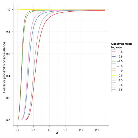
Figure 3: Posterior probability of equivalence versus variance of the mean log ratio, $\sigma_{i}^{2}$, for the given mean log ratio value.

A scatter plot of the estimated posterior probability of equivalence versus the observed mean log ratio is shown in Figure 4 with the genes separated by spot type. The values of the hyperparameters used to calculate the posterior probabilities are given in Table 4 of Appendix 1, and are the same as the values used for Figure 3.

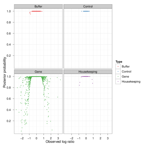
Figure 4: Posterior probability of equivalence versus observed mean log ratio for the stem cell genes: day 3 compared to day 0.

We note firstly that there are $327$ housekeeping genes spotted on the microarray, the most common nucleotide being NM_008084 for which there are $232$ spots. This nucleotide is a fragment of the gene glyceraldehyde-3-phosphate dehydrogenase (Gapdh) which has been validated as a good housekeeping gene in the mouse embryo (Mamo et al., 2007; Willems et al., 2006). Housekeeping genes are highly and constantly expressed across hybridisations, and are useful for quality assurance purposes, among other things. Of the total $327$ housekeeping spots, $316$ ($96.64$%) have a posterior probability of equivalence greater than $0.9999$, whilst all $232$ of the NM_008084 spots have posterior probability of equivalence greater than $0.9999925$.

The buffer and control genes are expected to have zero gene expression on both days, and are also equivalently expressed with high posterior probability, as expected.

Next, we observe some genes with observed mean log ratios lying outside the equivalence neighbourhood $(-1,1)$, but with posterior probabilities of equivalence close to one. There are $231$ genes in total with observed mean log ratios lying outside of the equivalence neighbourhood, with corresponding posterior probabilities of equivalence lying between $0.01665$ and $0.99779$. Of these $231$ genes, $22$ have a posterior probability of equivalence greater than $0.99$ and all also have a mean log ratio variance greater than $0.2228$. This is a large observed variance, as only $2$% of all genes on the microarray have an observed variance greater than $0.2228$, and explains the high posterior probability of equivalence for these genes, as indicated in Figure 3.

In Tuke et al. (2009), the authors identified, with gene profiling, 15 nucleotides whose observed expression levels over time correspond to the pre-specified profile referred to as the Oct4 profile. These nucleotides and associated gene are shown in Table 2 along with their observed posterior probability of equivalence. The Oct4 profile requires the nucleotides to have equivalent expression at day 3 compared to day 0 and so we expected that these nucleotides would have a posterior probability of equivalence close to one as seen in the table.

Nucleotide	Posterior Probability
NM_013633 (Oct4)	0.998
NM_009482 (Utfl)	0.9989
NM_011562 (Tdgf1)	0.9983
AK005182 (Slc35f2)	0.9992
NM_009426 (Trh)	0.9985
NM_010425 (Foxd3)	0.9993
AF246632 (Musd1)	0.9988
BC004805 (Skil)	0.9986
NM_010127 (Pou6f1)	0.9988
NM_007974 (Par2)	0.9974
AK010332 (Nanog)	0.9966
NM_007515 (Slc7a3)	0.9986
NM_010316 (Gng3)	0.9994
NM_011386 (Skil)	0.9986
NM_007905 (Rae-28)	0.9996

Table 2: Nucleotides identified by gene profiling with the Oct4 profile (Tuke et al., 2009) and their associated posterior probability of equivalence.

Figure 5 plots the estimated $q$-values (9) versus the posterior probabilities of equivalence for the stem cell mean log ratios comparing day 3 to day 0, and shows good concordance. We observe that as the posterior probability of equivalence decreases, the $q$-value increases to a maximum of 0.003069. This small observed maximum $q$-value is because the majority of genes are expected to be equivalently expressed between day 3 and day 0 and so even if all genes are considered equivalent then the expected proportion of false positives will be small.

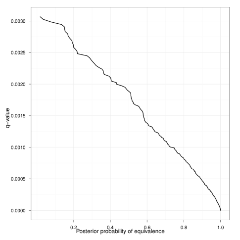
Figure 5: Estimated $q$-value versus posterior probability of equivalence for the stem cell data: day 3 compared to day 0.

5 Conclusion

We have shown in a general setting that the $q$-value, when represented as a posterior probability, satisfies some basic consistency requirements needed for any credible measure of evidence for equivalence. In particular, the $q$-value increases monotonically with the variance of the estimator. Importantly, we have established that the $P$-value does not satisfy these requirements, and hence should not be used as a measure of evidence for equivalence. Our results also demonstrate that any attempt to adapt Storey’s approach to estimating $q$-values from $P$-values in the equivalence testing context is logically untenable, and propose a simple alternative estimate. We note that the lack of duality between $P$-values and $q$-values in equivalence testing provides some fuel to the debate on the $P$-value as a measure of evidence per se, but discussion on this point is beyond the scope of the present paper.

It is worth remarking here that via simulations conducted (but not shown), the empirical Bayesian model we assumed of a mixture of three normal distributions provides a reasonable approximation to the true posterior probability of equivalence, even in situations where the true prior distribution of the parameter of interest deviates considerably from a mixture model of three normals.

6 Bibliography

Appendix 1: Estimation of hyperparameters using the EM algorithm

Applying the EM algorithm to the full probability model (11) for the observed mean log ratios, $Y_{i}$, we introduce the Bernoulli random variables $R_{i1},R_{i2}$ and $R_{i3}$, $i=1,\ldots,23040$, that are unobserved in the data.

The complete likelihood for the observed data vector $\boldsymbol{Y}$ and the unobserved data $\boldsymbol{R_{1}},\boldsymbol{R_{2}}$ and $\boldsymbol{R_{3}}$ is then

$$L(\boldsymbol{\Psi}|\boldsymbol{Y},\boldsymbol{R_{1}},\boldsymbol{R_{2}},\boldsymbol{R_{3}})=\prod^{23040}_{i=1}\prod^{3}_{j=1}\left[\pi_{j}g_{j}(y_{i},\mu_{j},\tau^{2}_{j})\right]^{R_{ij}},$$

where

$$g_{j}(y_{i},\mu_{j},\tau^{2}_{j})=\frac{1}{\sqrt{2\pi(\tau^{2}_{j}+\sigma^{2}_{i})}}\exp\left\{-\frac{(y_{i}-\mu_{j})^{2}}{2(\tau^{2}_{j}+\sigma^{2}_{i})}\right\},j=1,2,3,$$

$\sum_{j=1}^{3}\pi_{j}=1$, and $\boldsymbol{\Psi}=(\pi_{1},\pi_{2},\pi_{3},\mu_{1},\mu_{2},\mu_{3},\tau^{2}_{1},\tau^{2}_{2},\tau^{2}_{3})$.

That is, the log-likelihood is

$$\ell(\boldsymbol{\Psi}|\boldsymbol{Y},\boldsymbol{R_{1}},\boldsymbol{R_{2}},\boldsymbol{R_{3}})= \sum^{23040}_{i=1}\sum_{j=1}^{3}R_{ij}\log\pi_{j}+R_{ij}\log g_{i}(y_{i},\mu_{j},\tau^{2}_{j})$$ (15)

For exponential family distributions, the conditional expectation of the complete log likelihood $Q(\boldsymbol{\Psi}|\boldsymbol{\Psi}_{n})$, conditional on the estimated value $\boldsymbol{\Psi}_{n}$ of $\boldsymbol{\Psi}$ at the $n$th step, can be calculated by substituting $E[\boldsymbol{Z}|\boldsymbol{Y},\boldsymbol{\Psi}_{n}]$ in place of $\boldsymbol{Z}$, where $\boldsymbol{Z}$ represents the missing data (Dempster et al., 1977). For the observed mean log ratio for gene $i$,

$$E[R_{ij}|\boldsymbol{Y},\boldsymbol{\Psi_{n}}] =P(R_{ij}=1|\boldsymbol{Y},\boldsymbol{\Psi_{n}})$$

$$=\frac{\pi^{(n)}_{j}g_{j}(y_{i},\mu_{j}^{(n)},\tau^{2(n)}_{j})}{\sum_{j=1}^{3}\pi^{(n)}_{j}g_{j}(y_{i},\mu_{j}^{(n)},\tau^{2(n)}_{j})},$$

where the superscript $(n)$ indicates the parameter estimate from iteration $n$ of the EM algorithm. Substituting $\gamma_{ij}=E[R_{ij}|\boldsymbol{Y},\boldsymbol{\Psi_{n}}]$ in place of $R_{ij}$ in Equation (15) gives

$$Q(\boldsymbol{\Psi}|\boldsymbol{\Psi_{n}})= E[\log f(\boldsymbol{X}|\boldsymbol{\Psi})|\boldsymbol{Y},\boldsymbol{\Psi_{n}}]$$

$$= \sum^{23040}_{i=1}\sum_{j=1}^{3}\gamma_{ij}\log\pi_{j}+\gamma_{ij}\log g_{j}(y_{i},\mu_{j},\tau^{2}_{j})$$ (16)

In the maximisation step, we use a modification of the EM algorithm known as the Expectation/Conditional Maximisation (CEM) (Meng and Rubin, 1993). Here, the CEM replaces the M-step with a sequence of conditional maximisation steps so that the function $Q(\boldsymbol{\Psi}|\boldsymbol{\Psi_{n}})$ is maximised for each parameter in turn, whilst keeping the remaining parameters fixed.

Maximisation of $Q(\boldsymbol{\Psi}|\boldsymbol{\Psi_{n}})$ with respect to $\pi_{j}$, $j=1,2,3$, with the constraint $\sum_{j=1}^{3}\pi_{j}=1$, gives the parameter estimates for $\pi_{j}$ at the $(n+1)^{th}$ step as

$$\hat{\pi}_{j}^{(n+1)}=\frac{\sum^{23040}_{i=1}\gamma_{ij}}{\sum^{23040}_{i=1}\sum_{j=1}^{3}\gamma_{ij}},\quad j=1,2,3.$$

Maximisation of $Q(\boldsymbol{\Psi}|\boldsymbol{\Psi_{n}})$ with respect to $\mu_{j}$ gives the parameter estimates for $\mu_{j}$ at the $(n+1)^{th}$ step as

$$\hat{\mu}_{j}^{(n+1)}=\frac{\sum^{23040}_{i=1}\gamma_{ij}y_{i}/(\sigma^{2}_{i}+\hat{\tau}^{2(n)}_{j})}{\sum^{23040}_{i=1}\gamma_{ij}/(\sigma^{2}_{i}+\hat{\tau}^{2(n)}_{j})},\quad j=1,2,3.$$

Note the use of the estimates from the previous M-step for $\tau^{2}_{j}$, $j=1,2,3$.

Numerical methods: We used numerical optimisation, in particular, the R (R Development Core Team, 2011) function optimise (Brent, 2002) to find the values of $\tau^{2}_{j}$ that maximise $\sum_{i=1}^{23040}\gamma_{ij}g_{j}(y_{i},\mu^{(n+1)}_{j},\tau^{2}_{j})$ for $j=1,2,3$. The R function optimise uses a combination of golden section search and successive parabolic interpolation to find the maximum over an interval. We considered the interval $0\leq\tau^{2}_{j}\leq\max(\sigma^{2}_{i})$, $i=1,\ldots,23040;j=1,2,3$. Note again the use of the $(n+1)^{th}$ parameter estimate for $\mu_{j}$.

Choosing initial parameter values: We modified a method proposed by Finch et al. to obtain initial estimates of the hyperparameters given an initial choice of the mixing proportions $\pi_{j}$, $j=1,2,3$ for the EM algorithm. For each gene, there are two observations: the mean log ratio $y_{i}$ and the variance $\sigma^{2}_{i}$. These pairs of observations were ordered according to the mean log ratios $y_{i}$. These values were then split into three samples consisting of the smallest $n_{1}$ observations, the smallest $n_{2}$ of the remaining observations, and the remaining observations, where $n_{1}$ is the value $23040\pi_{1}$ rounded to the nearest integer and $n_{2}$ is the value $23040\pi_{2}$ rounded to the nearest integer. For each of these three samples, the estimate of $\mu_{j}$ was initialised as the sample mean of the observed mean log ratios. The initial value of $\tau^{2}_{j}$ was obtained by finding the value $\tau^{2}_{j}$ that maximises

$$\sum_{i=1}^{n_{j}}\log\left[\frac{1}{\sqrt{2\pi(\tau^{2}_{j}+\sigma^{2}_{i})}}\exp\left\{-\frac{(y_{i}-\hat{\mu}_{j})^{2}}{2(\tau^{2}_{j}+\sigma^{2}_{i})}\right\}\right],$$

where $n_{j}$ is the number of observations in the $j$th sample, $y_{i}$ and $\sigma^{2}_{i}$ are the pair of observations for each gene in the $j$th sample, and $\hat{\mu}_{j}$ is the sample mean of the $y_{i}$ in the $j$th sample. The R function optimise was used to find this maximum over the range $0\leq\tau^{2}_{j}\leq\max(\sigma^{2}_{i}),i=1,\ldots,n_{j}$, $j=1,2,3$.

Karlis and Xekalaki (2003) compare via simulations a number of methods for choosing initial values for the EM algorithm, including the one proposed by Finch et al. (1989). They observed that for two-component and three-component mixtures with equal mixing proportions for the initial values, Finch et al.’s method generally locates the ‘global maximum’ more often than other methods considered. They recommend that a mixed strategy is used in the choice of initial values in the EM algorithm, as different initial values may find a local but not a global maximum.

For each choice of initial parameter values, the EM algorithm is iterated for a limited number of steps. The EM algorithm is then run with the initial parameter values that give the largest likelihood for the initial iterations. In this final iteration, the EM algorithm is iterated until a high level of accuracy in the parameter estimates is achieved.

For the stem cell data, the initial values for the seven main mixing proportions considered are set out in Table 3. These are: equally contributing normals (Run 1); a single dominating normal (Runs 2, 3 and 4); and two dominating normals (Runs 5, 6 and 7). For each choice of the initial parameters, the EM algorithm was run for a limited number of steps, and the choice of initial parameters which produced the maximum log-likelihood was then repeated for a larger number of iterations.

Run	Initial $\pi_{1}$	Initial $\pi_{2}$	Initial $\pi_{3}$
1	0.33	0.33	0.33
2	0.8	0.1	0.1
3	0.1	0.8	0.1
4	0.1	0.1	0.8
5	0.1	0.45	0.45
6	0.45	0.1	0.45
7	0.45	0.45	0.1

Table 3: Initial mixing proportion for EM algorithm.

After each iteration of the EM algorithm, the absolute difference in each of the parameter estimates compared to the previous iteration was calculated, and the iterations continued until the maximum of these differences was less than $10^{-5}$. The top five runs ordered by log-likelihood showed consistent parameter estimates, and the initial values, $\pi_{1}=0.45,\pi_{2}=0.1,\pi_{3}=0.1$, produced the maximum log-likelihood of $5368.77$. These estimates were then used for the initial values of the EM algorithm which was repeated until the maximum difference in consecutive parameter estimates was less than $10^{-10}$.

The resulting final parameter estimates for the stem cell data are given in Table 4.

Parameter	Estimate
$\pi_{1}$	0.03177
$\pi_{2}$	0.3576
$\pi_{3}$	0.6107
$\mu_{1}$	-0.09135
$\mu_{2}$	-0.01845
$\mu_{3}$	0.008169
$\tau_{1}^{2}$	0.3558
$\tau_{2}^{2}$	0.01958
$\tau_{3}^{2}$	5.426e-12

Table 4: Parameter estimates from the EM algorithm for stem cell data.

Appendix 2: Monotonicity of posterior probabilities of equivalence

Lemma 1: Suppose $f(x)$ is a symmetric function with $f(x)>0$ for all $x$ and consider numbers $a,b,c,d,\ell$ with $-\ell<a<b<\ell$, $0<c$, $\ell<d$ and $b-a=d-c$. Then

$$\frac{\int_{a}^{b}x^{2}f(x)dx}{\int_{a}^{b}f(x)dx}<\frac{\int_{c}^{d}x^{2}f(x)dx}{\int_{c}^{d}f(x)dx}$$

Proof.

By symmetry, we can assume $b>0$ and $|a|\leq|b|$. It is then sufficient to consider the following three cases.

1. Case 1:$b\leq c$: Observe that

   $$\frac{\int_{a}^{b}x^{2}f(x)dx}{\int_{a}^{b}f(x)dx}<b^{2}\mbox{ and }\frac{\int_{c}^{d}x^{2}f(x)dx}{\int_{c}^{d}f(x)dx}>c^{2}$$

   so the result follows.

2. Case 2:$c<b$ and $|a|\leq c$:
   Let

   $$m_{1}=\frac{\int_{a}^{c}x^{2}f(x)dx}{\int_{a}^{c}f(x)dx},\ m_{2}=\frac{\int_{c}^{b}x^{2}f(x)dx}{\int_{c}^{b}f(x)dx}\mbox{ and }m_{3}=\frac{\int_{b}^{d}x^{2}f(x)dx}{\int_{b}^{d}f(x)dx}$$

   and observe that $m_{1}<c^{2}<m_{2}<b^{2}<m_{3}$. Since

   $$\frac{\int_{a}^{b}x^{2}f(x)dx}{\int_{a}^{b}f(x)dx}$$

   is a weighted average of $m_{1}$ and $m_{2}$ and

   $$\frac{\int_{c}^{d}x^{2}f(x)dx}{\int_{d}^{d}f(x)dx}$$

   is a weighted average of $m_{2}$ and $m_{3}$, the result follows.

3. Case 3: $c<b$ and $|a|>c$:
   To have $|a|>c$ requires $a$ to be negative. Now let

   $$m_{1}=\frac{\int_{a}^{-c}x^{2}f(x)dx}{\int_{a}^{-c}f(x)dx},\ m_{0}=\frac{\int_{-c}^{c}x^{2}f(x)dx}{\int_{-c}^{c}f(x)dx},\ m_{2}=\frac{\int_{c}^{b}x^{2}f(x)dx}{\int_{c}^{b}f(x)dx}$$

   $$\mbox{ and }\ m_{3}=\frac{\int_{b}^{d}x^{2}f(x)dx}{\int_{b}^{d}f(x)dx},$$

   and observe $m_{0}<c^{2}<m_{1}<m_{2}<b^{2}<m_{3}$. Since

   $$\frac{\int_{a}^{b}x^{2}f(x)dx}{\int_{a}^{b}f(x)dx}$$

   is a weighted average of $m_{0},\ m_{1}$ and $m_{2}$ and

   $$\frac{\int_{c}^{d}x^{2}f(x)dx}{\int_{d}^{d}f(x)dx}$$

   is a weighted average of $m_{2}$ and $m_{3}$, the result follows.

∎

Theorem 2: Suppose $\theta$ has prior distribution $P(\theta)$ and $T|\theta\sim N(\theta,\sigma^{2})$. Consider numbers $0<\ell<\varepsilon$ and assume further that $0<P(-\varepsilon<\theta<\varepsilon)<1$. Then $P(-\varepsilon<\theta<\varepsilon\mid-\ell<T<\ell)$ is a decreasing function of $\sigma^{2}$.

Proof.

Observe that

$$P(-\varepsilon<\theta<\varepsilon\mid-\ell<T<\ell) = \frac{\int_{|\theta|\leq\varepsilon}P(\theta)\int_{-\ell}^{\ell}e^{-\frac{1}{2\sigma^{2}}(t-\theta)^{2}}dtd\theta}{\int_{-\infty}^{\infty}P(\theta)\int_{-\ell}^{\ell}e^{-\frac{1}{2\sigma^{2}}(t-\theta)^{2}}dtd\theta}$$

$$= \frac{\int_{|\theta|\leq\varepsilon}P(\theta)\int_{-\ell-\theta}^{\ell-\theta}e^{-\frac{1}{2\sigma^{2}}y^{2}}dyd\theta}{\int_{\theta\leq\varepsilon}P(\theta)\int_{-\ell-\theta}^{\ell-\theta}e^{-\frac{1}{2\sigma^{2}}y^{2}}dyd\theta+\int_{|\theta|>\varepsilon}P(\theta)\int_{-\ell-\theta}^{\ell-\theta}e^{-\frac{1}{2\sigma^{2}}y^{2}}dyd\theta}.$$

Taking $\omega=1/(2\sigma^{2})$, it is sufficient to show that the posterior odds

$$r(\omega)=\frac{\int_{|\theta|\leq\varepsilon}P(\theta)\int_{-\ell-\theta}^{\ell-\theta}e^{-\omega y^{2}}dyd\theta}{\int_{|\theta|>\varepsilon}P(\theta)\int_{-\ell-\theta}^{\ell-\theta}e^{-\omega y^{2}}dyd\theta}.$$

is increasing in $\omega$. Now observe

$$r^{\prime}(\omega) = \left\{\left(\int_{|\theta|\leq\varepsilon}P(\theta)\int_{-\ell-\theta}^{\ell-\theta}e^{-\omega y^{2}}dyd\theta\right)\left(\int_{|\theta|>\varepsilon}P(\theta)\int_{-\ell-\theta}^{\ell-\theta}y^{2}e^{-\omega y^{2}}dyd\theta\right)\right.$$

$$-\left.\left(\int_{|\theta|\leq\varepsilon}P(\theta)\int_{-\ell-\theta}^{\ell-\theta}y^{2}e^{-\omega y^{2}}dyd\theta\right)\left(\int_{|\theta|>\varepsilon}P(\theta)\int_{-\ell-\theta}^{\ell-\theta}e^{-\omega y^{2}}dyd\theta\right)\right\}$$

$$\bigg{/}\left\{{\int_{|\theta|>\varepsilon}P(\theta)\int_{-\ell-\theta}^{\ell-\theta}e^{-\omega y^{2}}dyd\theta}\right\}^{2}.$$

Taking

$$A_{1}=\inf_{|\theta|>\epsilon}\frac{\int_{-\ell-\theta}^{\ell-\theta}y^{2}e^{-\omega y^{2}}dy}{\int_{-\ell-\theta}^{\ell-\theta}e^{-\omega y^{2}}dy}\mbox{ and }A_{0}=\sup_{|\theta|\leq\epsilon}\frac{\int_{-\ell-\theta}^{\ell-\theta}y^{2}e^{-\omega y^{2}}dy}{\int_{-\ell-\theta}^{\ell-\theta}e^{-\omega y^{2}}dy},$$

it follows that

$$r^{\prime}(\omega)\geq(A_{1}-A_{0})\frac{\left(\int_{|\theta|\leq\varepsilon}P(\theta)\int_{-\ell-\theta}^{\ell-\theta}e^{-\omega y^{2}}dyd\theta\right)\left({\int_{|\theta|>\varepsilon}P(\theta)\int_{-\ell-\theta}^{\ell-\theta}e^{-\omega y^{2}}dyd\theta}\right)}{\left\{{\int_{|\theta|>\varepsilon}P(\theta)\int_{-\ell-\theta}^{\ell-\theta}e^{-\omega y^{2}}dyd\theta}\right\}^{2}}$$

By Lemma 1, $A_{1}>A_{0}$ so the proof is complete. ∎

References

- Brent (2002) Brent, R. P. Algorithms for Minimization Without Derivatives. Dover Pubns, 2002.
- Casella and Berger (2002) Casella, G. and Berger, R. L. Statistical Inference. Duxbury Advanced Series in Statistics and Decision Sciences. Thomson Learning, 2002.
- Chow and Liu (2008) Chow, S. C. and Liu, J. Design and Analysis of Bioavailability and Bioequivalence Studies. Chapman & Hall/CRC Biostatistics Series. CRC Press, 2008.
- Dempster et al. (1977) Dempster, A., Laird, N., and Rubin, D. Maximum likelihood from incomplete data via the EM algorithm. Journal of the Royal Statistical Society. Series B (Methodological), pages 1–38, 1977.
- Finch et al. (1989) Finch, S. J., Mendell, N. R., and Thode, H. C. Probabilistic Measures of Adequacy of a Numerical Search for a Global Maximum. Journal of the American Statistical Association, 84(408):1020–1023, 1989.
- Ge et al. (2003) Ge, Y., Dudoit, S., and Speed, T. P. Resampling-Based Multiple Testing for Microarray Data Analysis. TEST, 12(1):1–77, 2003.
- Gelman (2004) Gelman, A. Bayesian data analysis. Texts in statistical science. Chapman & Hall/CRC, 2004.