A novel technique for measuring masses of a pair of semi-invisibly decaying particles

Abstract

Motivated by evidence for the existence of dark matter, many new physics models predict the pair production of new particles, followed by the decays into two invisible particles, leading to a momentum imbalance in the visible system. For the cases where all four components of the vector sum of the two ‘missing’ momenta are measured from the momentum imbalance, we present analytic solutions of the final state system in terms of measureable momenta, with the mass shell constraints taken into account. We then introduce new variables which allow the masses involved in the new physics process, including that of the dark matter particles, to be extracted. These are compared with a selection of variables in the literature, and possible applications at lepton and hadron colliders are discussed.

Introduction.— If new physics (NP) is observed in collider experiments, the mass of the NP particles involved will be the first quantities to be measured. Motivated by the astrophysical evidence of dark matter, many theories beyond the Standard Model (SM) include a neutral dark matter (DM) candidate as the lightest of the new particles. In many of these models, the stability of the DM against decays into SM particles is enforced by a new (discrete) symmetry. Typically such symmetry implies that NP particles are pair produced in a collider, which subsequently cascade decay into a pair of DM particles that escape detection. An example is the minimal supersymmetric extension of the SM (MSSM) with R-parity.

A possible collider process is shown schematically in Fig. 1. The NP particle $X/X^{\prime}$ decays via (a system of) visible particle(s) $Y/Y^{\prime}$ into the DM particle $N/N^{\prime}$. The momenta of these particles are denoted $p_{i=X,X^{\prime},Y,Y^{\prime},N,N^{\prime}}$. If $p_{N}$ and $p_{N^{\prime}}$ could be measured directly, the true masses ${\bf m}^{\rm true}\equiv(m_{N},m_{X})$ for the particles $N/N^{\prime}$ and $X/X^{\prime}$ would show up as delta-function peaks in the invariant mass distributions of $p_{N}/p_{N^{\prime}}$ and $p_{X}/p_{X^{\prime}}$ in the limit of zero width and perfect detector resolution. In reality, at best the vector sum $p\hskip-4.49997pt/=p_{N}+p_{N^{\prime}}$ may be inferred from the 4-momentum imbalance between the initial state and observed final state particles. An observed event is then defined by the 4-momenta set ${\mathbf{p}}\equiv\{p_{Y},p_{Y^{\prime}},p\hskip-4.49997pt/\}$. Although ${\bf m}^{\rm true}$ cannot be measured directly, including mass shell conditions consistent with the topology in Fig. 1 constrains the mass hypothesis $\tilde{\bf{m}}\equiv(\tilde{m}_{N},\tilde{m}_{X})$ consistent with ${\mathbf{p}}$ and improves the determination of ${\bf m}^{\rm true}$. Systematically incorporating these constraints would hence be beneficial.

In this Letter, we describe a method to determine all possible $\tilde{\bf{m}}$ which takes into account the mass shell constraints when ${\mathbf{p}}$, in particular all four components of $p\hskip-4.49997pt/$, is known, such as at a future linear collider, and in central exclusive production processes at the LHC with tagged forward protons. For each $\tilde{\bf{m}}$ we obtain analytic solutions for the momenta $p_{i}$. Using the fact that ${\bf m}^{\rm true}$ lies within the boundary of $\tilde{\bf{m}}$, we define boundary variables $\tilde{\bf{m}}^{\rm max}\equiv(\tilde{m}_{N}^{\rm max},\tilde{m}_{X}^{\rm max})$ which develop sharp edges at ${\bf m}^{\rm true}$ without further input.

To illustrate the use of these variables, we will use the example of selectron pair production in the MSSM to demonstrate how they complement existing ‘standard’ mass measurement techniques at future linear colliders, many of which however do not include information from the mass shell constraints. As the edges of $\tilde{\bf{m}}^{\rm max}$ are independent of the system centre of mass energy ($\sqrt{s}$), they can be particularly useful at the Large Hadron Collider (LHC). We will briefly discuss how our methods can be used in central exclusive processes, and connections with ‘transverse’ variables in inelastic processes at the LHC.

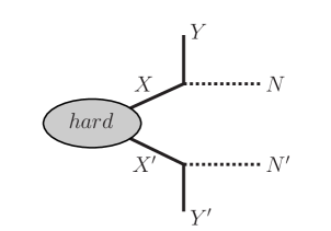
Figure 1: The event topology. $Y/Y^{\prime}$ are visible, and their 4-momenta can be directly observed. $N/N^{\prime}$ are dark matter candidates; only the vector sum of their 4-momenta could be inferred from the momentum imbalance between the initial and observed final state particles.

The calculation method.— Given a set of measurable 4-momenta ${\mathbf{p}}$, the 4-momenta of the particles $N,N^{\prime},X$ and $X^{\prime}$ in Fig. 1 can be parametrised as

$$p_{N/N^{\prime}} = \frac{1\mp a}{2}p\hskip-4.49997pt/\pm\frac{b}{2}p_{Y}\mp\frac{c}{2}p_{Y^{\prime}}\pm dP\,,$$ (1)

$$p_{X/X^{\prime}} = p_{N/N^{\prime}}+p_{Y/Y^{\prime}}\,,$$ (2)

for dimensionless constants $a,b,c,d$, which includes the missing momentum constraint $p\hskip-4.49997pt/=p_{N}+p_{N^{\prime}}$ by construction. In Eq. (1), the four basis momentum vectors are given by ${\mathbf{p}}$ and $P$, the latter of which is a space-like vector defined by $P_{\mu}\equiv\epsilon_{\mu\nu\rho\sigma}p\hskip-4.49997pt/^{\nu}p_{Y}^{\rho}p_{Y^{\prime}}^{\sigma}$. As we shall see, the space-like nature of $P$ allows consistent solutions to be classified using a simple criterion.

The (equal) mass shell constraints are given by

$$\tilde{m}_{N}^{2}=p^{2}_{N}=p^{2}_{N^{\prime}}\,,\qquad\tilde{m}_{X}^{2}=p^{2}_{X}=p^{2}_{X^{\prime}}\,,$$ (3)

where $\tilde{\bf{m}}\equiv(\tilde{m}_{N},\tilde{m}_{X})$ are test mass values which need not coincide with the true masses ${\bf m}^{\rm true}\equiv(m_{N},m_{X})$. Given $\tilde{\bf{m}}$, the coefficients $(a,b,c,d)$ can be determined by the four mass shell conditions. In fact, using $P\cdot p\hskip-4.49997pt/=P\cdot p_{Y}=P\cdot p_{Y^{\prime}}=0$, three equations linear in $(a,b,c)$ but independent of $d$ can be obtained by considering the three squared mass differences $(p_{N}^{2}-p_{N^{\prime}}^{2},p_{X}^{2}-p_{N}^{2},p_{X^{\prime}}^{2}-p_{N^{\prime}}^{2})$. Define the Lorentz invariants

$${\bf\Lambda}\equiv(\lambda_{p\hskip-3.14998pt/^{2}},\lambda_{p\hskip-3.14998pt/p_{Y}},\lambda_{p\hskip-3.14998pt/p_{Y^{\prime}}},\lambda_{p_{Y}^{2}},\lambda_{p_{Y^{\prime}}^{2}})\equiv(\alpha,\beta,\beta^{\prime},\epsilon,\epsilon^{\prime})\,,$$ (4)

where $\lambda_{p_{i}p_{j}}\equiv p_{i}\cdot p_{j}/p_{Y}\cdot p_{Y^{\prime}}$ and $\lambda_{p_{i}^{2}}\equiv p^{2}_{i}/p_{Y}\cdot p_{Y^{\prime}}$. The solution for $(a,b,c)$ is then given by

$$a = \frac{1}{{\mathcal{M}}}\left[\epsilon\beta^{\prime}(1+\beta^{\prime})-\epsilon^{\prime}\beta(1+\beta)-\epsilon\epsilon^{\prime}(\beta-\beta^{\prime})\right]$$ (5)

$$+\frac{\lambda_{\Delta}}{{\mathcal{M}}}\left[\beta(1+\epsilon^{\prime})-\beta^{\prime}(1+\epsilon)\right]\,,$$

$$b = \frac{1}{{\mathcal{M}}}\left[\epsilon(1+\beta^{\prime})(\beta^{\prime 2}-\epsilon^{\prime}\alpha)+\epsilon^{\prime}(1+\beta)(\beta\beta^{\prime}-\alpha)\right]$$ (6)

$$+\frac{\lambda_{\Delta}}{{\mathcal{M}}}\left[\alpha(1+\epsilon^{\prime})-\beta^{\prime}(\beta+\beta^{\prime})\right]+\beta^{\prime}\,,$$

$$c = \frac{1}{{\mathcal{M}}}\left[\epsilon^{\prime}(1+\beta)(\beta^{2}-\epsilon\alpha)+\epsilon(1+\beta^{\prime})(\beta\beta^{\prime}-\alpha)\right]$$ (7)

$$+\frac{\lambda_{\Delta}}{{\mathcal{M}}}\left[\alpha(1+\epsilon)-\beta(\beta^{\prime}+\beta)\right]+\beta\,,$$

where $\lambda_{\Delta}\equiv\lambda_{\tilde{m}_{X}^{2}}-\lambda_{\tilde{m}_{N}^{2}}$, and

$${\mathcal{M}}=2\beta\beta^{\prime}-\alpha(1-\epsilon\epsilon^{\prime})-\epsilon\beta^{\prime 2}-\epsilon^{\prime}\beta^{2}$$ (8)

is the determinant involved when inverting the system of three linear equations. Inserting these solutions back into the mass shell constraints leads to the equation

$$\lambda_{\tilde{m}_{N}^{2}} = \frac{c_{a}}{4{\mathcal{M}}}\lambda_{\Delta}^{2}+\frac{c_{b}}{2{\mathcal{M}}}\lambda_{\Delta}+\frac{c_{c}}{4{\mathcal{M}}}+d^{2}\lambda_{P^{2}}\,.$$ (9)

This is our main result, from which all variables of interest that we discuss below can be derived. The coefficients are given by

$$c_{a} = \alpha(2+\epsilon+\epsilon^{\prime})-(\beta+\beta^{\prime})^{2}\,,$$ (10)

$$c_{b} = (\beta+\beta^{\prime})\left[(\beta+\epsilon)\beta^{\prime}+(\beta^{\prime}+\epsilon^{\prime})\beta\right]$$ (11)

$$-\alpha[(\beta+\epsilon)(1+\epsilon^{\prime})+(\beta^{\prime}+\epsilon^{\prime})(1+\epsilon)]\,,$$

$$c_{c} = -\alpha^{2}(1-\epsilon\epsilon^{\prime})-\left[2\beta\beta^{\prime}+\epsilon\beta^{\prime}+\epsilon^{\prime}\beta\right]^{2}+4\alpha\beta\beta^{\prime}$$ (12)

$$+\alpha\left[\epsilon^{\prime}(1+\epsilon)(2\beta+\epsilon)+\epsilon(1+\epsilon^{\prime})(2\beta^{\prime}+\epsilon^{\prime})\right].~{}~{}$$

A hypothesis $\tilde{\bf{m}}$ is consistent if the corresponding $\lambda_{\Delta}$ and $\lambda_{\tilde{m}_{N}^{2}}$ lead to $d^{2}>0$ in Eq. (9). In this case a two fold degenerate solution for $p_{i}$ with unique $(a,b,c)$ and $d=\pm\sqrt{d^{2}}$ is obtained.

We have therefore found a simple criterion to determine the consistency of $\tilde{\bf{m}}$ with a given ${\mathbf{p}}$, and solve for $p_{i}$ explicitly in terms of the Lorentz invariants ${\bf\Lambda}$. More observations on the properties of the solutions can be made. First, the sign of the energy component of the two solutions (for $\pm\sqrt{d^{2}}$) must be the same, since it is always possible to boost to a frame where the energy component of the space-like vector $P$ is zero, in which case the two solutions have the same energies. Second, since the consistent solutions are continuous functions of $\tilde{m}_{N}$ and $\tilde{m}_{X}$, the energies of all consistent solutions must have the same sign. The energies must then be positive because ${\bf m}^{\rm true}$ is a consistent solution.

It can be shown that $c_{a}/4{\mathcal{M}}<0$ in Eq. (9). Since $P$ is space-like, we have $\lambda_{P^{2}}<0$ and so on the $(\tilde{m}_{X}^{2}-\tilde{m}_{N}^{2},\tilde{m}_{N}^{2})$ plane, the consistent mass region is bounded from above by Eq. (9) with $d^{2}=0$. Also, it is bounded from below by $\tilde{m}_{N}^{2}>0$. This consistent mass region can be transformed into a corresponding region in the $\tilde{\bf{m}}$ space, which will be different for each event but will always include ${\bf m}^{\rm true}$ in the absence of detector smearing effects. A density plot for consistent mass hypothesis, which in principle includes all kinematic information, will develop a peaking structure around ${\bf m}^{\rm true}$ when a sufficient number of events are accumulated.

Since all solutions $p_{i}$ consistent with ${\mathbf{p}}$ can now be obtained for each event, our method provides a departure point for further analysis of the hard process. The simple consistent mass boundary also allows new kinematic variables characterising the mass scales of the system to be constructed without additional input such as $m_{N}$. In particular, the fact that the finite consistent mass region is characterised by the quadratic curve Eq. (9) implies that the maximum consistent values of $\tilde{\bf{m}}$, denoted by $\tilde{\bf{m}}^{\rm max}=(\tilde{m}_{N}^{\rm max},\tilde{m}_{X}^{\rm max})$, can be calculated unambiguously for each event. These quantities are given by

$$(\tilde{m}_{N}^{\rm max})^{2} = \frac{p_{Y}\cdot p_{Y^{\prime}}}{4{\mathcal{M}}}\left[c_{c}-\frac{c_{b}^{2}}{c_{a}}\right]\,,$$ (13)

$$(\tilde{m}_{X}^{\rm max})^{2} = \frac{p_{Y}\cdot p_{Y^{\prime}}}{4{\mathcal{M}}}\left[c_{c}-\frac{(c_{b}+2{\mathcal{M}})^{2}}{c_{a}}\right]\,.$$ (14)

By construction, they are greater than the true masses. Other variables defined on the boundary can also be constructed. For example, if particular values of $\tilde{m}_{N}$ are assumed, the extremal values of $\tilde{m}_{X}$, denoted $\tilde{m}_{X}^{\rm min,max}(\tilde{m}_{N})$, can be obtained using Eq. (9). For $\tilde{m}_{N}=m_{N}$, $\tilde{m}_{X}^{\rm min(max)}(m_{N})$ is smaller (larger) than $m_{X}$ by construction, with $m_{X}$ being the upper (lower) endpoint of the distributions. The relationship of these quantities in a ‘typical’ event is displayed in Fig. 2. Note that $\tilde{m}_{X}^{\rm min}(m_{N})$ corresponds to the quantity discussed in Ref. Feng:1993sd . Since its functional form is different from $\tilde{\bf{m}}^{\rm max}$, it contains in principle complementary information.

Although not considered in this Letter, the methods for finding consistent $\tilde{\bf{m}}$ and $\tilde{\bf{m}}^{\rm max}$ should be valid even when the equal mass constraints, Eq. (3), are relaxed. In this case Eq. (9) becomes a quadratic function of two or three independent mass differences, for the case of one or no pairs of equal-mass particles, respectively. A unique $\tilde{\bf{m}}^{\rm max}$, now containing three or four elements, can again be obtained analytically for each ${\mathbf{p}}$.

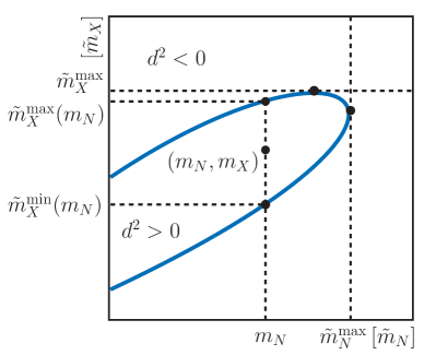
Figure 2: Consistent $(\tilde{m}_{N},\tilde{m}_{X})$ region for a ‘typical event’, defined by the 4-momenta $(p_{Y},p_{Y^{\prime}},p\hskip-4.49997pt/)$. The region $d^{2}>0$ is consistent. It includes the true mass point $(m_{N},m_{X})$. $\tilde{m}^{\rm max}_{N,X}$ are the maximum $\tilde{m}_{N}$/$\tilde{m}_{X}$ values, while $\tilde{m}_{X}^{\rm min,max}(m_{N})$ is the minimal/maximal value of $\tilde{m}_{X}$ given $m_{N}$.

Note that $\tilde{\bf{m}}^{\rm max}$ depends only on ${\mathbf{p}}$, and so while the shape of the distributions is sensitive to detailed dynamics and $\sqrt{s}$, the position of the edges are not. This should be compared with other linear collider mass measurement techniques which depend on $\sqrt{s}$ being controllable/fixed, without including mass shell constraints. For example, by varying $\sqrt{s}$, the threshold scanning method AguilarSaavedra:2001rg is sensitive to the production threshold scale $2m_{X}$, while directly measuring $2m_{N}$ will be challenging since $N/N^{\prime}$ are invisible. In addition, the distribution of $E_{Y/Y^{\prime}}$, the energy of $Y$ and $Y^{\prime}$, have endpoints Feng:1993sd ; hep-ph/9910416

$$E^{{\rm max,min}}_{Y/Y^{\prime}}=\frac{\sqrt{s}}{4}\left[1-\frac{m_{N}^{2}}{m_{X}^{2}}\right]\left[1\pm\sqrt{1-\frac{4m_{X}^{2}}{s}}\right]$$ (15)

when radiation and detector smearing effects are neglected. The true mass ${\bf m}^{\rm true}$ can then be obtained if the endpoints and $\sqrt{s}$ are accurately determined. Depending on the values of ${\bf m}^{\rm true}$ and $\sqrt{s}$, our method could have statistical advantages in the endpoint determination. Furthermore, the fact that the $\tilde{\bf{m}}^{\rm max}$ are bounded from below by ${\bf m}^{\rm true}$ implies that these variables could be particularly effective in separating the signal events from (the SM) background when used simultaneously. More interestingly, the $\sqrt{s}$ independence and Lorentz invariance of $\tilde{\bf{m}}^{\rm max}$ leads to the possibility of utilising these variables in hadron-hadron collisions at the LHC, where the partonic $\sqrt{s}$ cannot be controlled directly. We shall illustrate these points with the examples below.

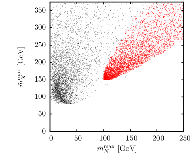
Figure 3: Scatter plot for $\tilde{\bf{m}}^{\rm max}=(\tilde{m}_{N}^{\rm max},\tilde{m}_{X}^{\rm max})$ for the SM leptonic $W^{+}W^{-}$ events (black), and pair production of selectrons ($m_{X}=150$ GeV) in MSSM, followed by decays into neutralinos ($m_{N}=100$ GeV) and electrons (red) at a 3 TeV $e^{+}e^{-}$ collider. 10,000 events for each process are displayed. No cuts, detector smearing and radiation effects are included.

Examples.— Our first example is based on a $e^{+}e^{-}$ collider with $\sqrt{s}=3$ TeV, the proposed CLIC energy CLIC . We use Herwig++ v2.5.0 Bahr:2008pv to simulate pair production of right handed selectrons ($\tilde{e}_{R}$) in MSSM, followed by decay into a pair of electrons and two lightest neutralino ($\tilde{\chi}$), assumed to be the superpartner of the SM $U(1)_{Y}$ gauge boson, and which is stable and escape detection:

$$e^{+}e^{-} \to \tilde{e}_{R}^{+}\tilde{e}_{R}^{-}\to e^{+}e^{-}\tilde{\chi}\tilde{\chi}\,.$$ (16)

The mass of $\tilde{e}_{R}$ ($m_{X}$) and $\tilde{\chi}$ ($m_{N}$) are chosen to be 150 and 100 GeV respectively. The small electron mass means that $\epsilon,\epsilon^{\prime}$ in Eq. (4) can be safely neglected, leading to much simplified analytic expressions. For comparison, the irreducible SM $W^{+}W^{-}$ background:

$$e^{+}e^{-} \to W^{+}W^{-}\to e^{+}e^{-}\nu\bar{\nu}\,,$$ (17)

is also simulated. The cross sections for the two processes are displayed in Table 1.

	SM	MSSM
($m_{N},m_{X}$) [GeV]	(0, 80.4)	(100, 150)
$\sigma_{\rm total}$ $[{\rm fb}]$	7	68

Table 1: Total cross sections for $e^{+}e^{-}+p\hskip-4.49997pt/$ events for the SM $W^{+}W^{-}$ and MSSM selectron pair production, followed by decays into electrons and neutralinos at a 3 TeV $e^{+}e^{-}$ collider. The $W\to e\nu_{e}$ branching ratio is taken as 0.108.

In Fig. 3, we show a scatter plot of $\tilde{\bf{m}}^{\rm max}$ for the MSSM (red) and SM (black) processes at parton level, i.e. without initial and final state photon radiation. While the cross section for the MSSM signal process is already an order of magnitude larger than the SM background, it is instructive to see that the two processes are cleanly separated before applying additional selection cuts. Given the simple mass dependence, we expect similar scatter plots to be also useful in separating different NP processes.

Next we present the $\tilde{m}_{N}^{\rm max}$, $\tilde{m}_{X}^{\rm max}$ and electron energy $E_{Y/Y^{\prime}}$ distributions for the MSSM sample in Fig. 4. In this particular sample, we see that at parton level there is a statistical gain of a factor of 2 to 3 near the endpoint of $\tilde{m}_{N}^{\rm max}$ and $\tilde{m}_{X}^{\rm max}$ over that of the $E_{Y/Y^{\prime}}$ distribution. While the large difference between $\sqrt{s}$ and $\tilde{\bf{m}}^{\rm max}$ results in the long tails for the $\tilde{\bf{m}}^{\rm max}$ distributions, the tails fall off sufficiently quickly and sharp edge structures remain at ${\bf m}^{\rm true}$. Note that the flat $E_{Y/Y^{\prime}}$ distribution is due to the spin-0 nature of the selectrons, and different spin assignments can lead to different (endpoint) distributions. Also, the small $4m_{X}^{2}/s$ ratio means that $E^{\rm min}_{Y/Y^{\prime}}$ is very close to zero, so this endpoint might not be measured if additional energy/momentum cuts were imposed.

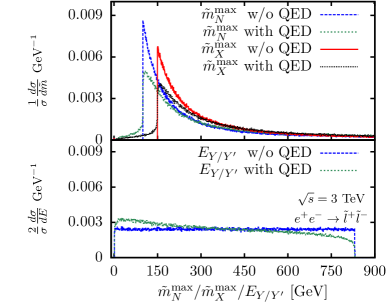
Figure 4: $\tilde{m}_{N}^{\rm max}$ (blue/green), $\tilde{m}_{X}^{\rm max}$ (red/black) and $E_{Y/Y^{\prime}}$ distributions for pair production of selectrons ($m_{X}=150$ GeV) in MSSM, followed by decays into electrons and neutralinos ($m_{N}=100$ GeV) at a 3 TeV $e^{+}e^{-}$ collider. Simulations both with and without the inclusion of QED radiation are displayed. No cuts and detector smearing effects are included.

When bremsstrahlung effects are included, all distributions are distorted. Now $p\hskip-4.49997pt/$ cannot be fully determined, in part due to initial state radiation down the beam pipe. The $p\hskip-4.49997pt/$ values needed for the more realistic distributions in Fig. 4 are obtained from the momentum imbalance between the final state and the initial state $e^{+}e^{-}$ systems, assuming no bremsstrahlung effects for the latter. Initial state radiation is calculable in perturbative QED, and its effect on the parton $\tilde{\bf{m}}^{\rm max}$ distributions may be incorporated in a more sophisticated treatment, which is beyond the scope of the present study. In our simple estimate, the $\tilde{\bf{m}}^{\rm max}$ distributions still display sharp edge structures around ${\bf m}^{\rm true}$ despite the radiation effects.

Next we turn to possible applications at the LHC. For central exclusive production (CEP) processes (see Ref. Albrow:2010yb and references therein for more details), for example two-photon production of a pair of charged particles ($X/X^{\prime}$)

$$pp \to p\,+\,\gamma\gamma\,+\,p$$ (18)

$$\phantom{p\,+\,\,\,\,}\gamma\gamma\to X^{(\pm)}X^{\prime(\mp)}\,,$$

followed by decays as depicted in Fig. 1, all four components of $p\hskip-4.49997pt/$ can be determined when the two final state protons are measured, which could be achieved by installing proton tagging detectors far from the interaction point Albrow:2008pn . In the first equation of Eq. (18), the ‘$+$’ signs represent the presence of rapidity gaps. Contrary to $e^{+}e^{-}$ processes, $\sqrt{s}$ is differerent for each CEP event. This means that the $E_{Y/Y^{\prime}}$ endpoint method cannot be directly used, while the $\tilde{\bf{m}}^{\rm max}$ method can. The invariant mass/energy of $\gamma\gamma$ and $p\hskip-4.49997pt/$, which have lower endpoints at $2m_{X}$ and $2m_{N}$ respectively, have been proposed to measure ${\bf m}^{\rm true}$ in CEP Schul:2008sr . Since $\tilde{\bf{m}}^{\rm max}$ takes the mass shell constraints into account, they are expected to have sharper distributions over the other variables. A comparison between these observables, and the precision on ${\bf m}^{\rm true}$ that can be achieved at the LHC using $\tilde{\bf{m}}^{\rm max}$ will be discussed in a separate article HarlandLang:2011ih .

Finally, for inelastic processes at the LHC, only the transverse components of $p\hskip-4.49997pt/$, i.e. $p\hskip-4.49997pt/_{T}$, might be measured. If only the short decay chain in Fig. 1 is observed, measuring ${\bf m}^{\rm true}$ will be challenging. In principle, ${\bf m}^{\rm true}$ could be measured from the kink structure of $m_{T2}^{\rm max}(\tilde{m}_{N})$ Lester:1999tx ; arXiv:0706.2871 ; arXiv:0910.3679 . However, the kink resides at the tail of the $m_{T2}(\tilde{m}_{N})$ distribution and so an accurate measurement will be difficult. In this case, the mass measurement in CEP could be crucial. It was shown in Ref. Cheng:2008hk that $m_{T2}(\tilde{m}_{N})$ is a boundary of the mass region consistent with the mass shell constraints. We have checked numerically that this corresponds to $\tilde{m}_{X}^{\rm min}(\tilde{m}_{N})$ over all physical $p\hskip-4.49997pt/$ configurations, given $p\hskip-4.49997pt/_{T}$. How solutions other than $\tilde{m}_{X}^{\rm min}(\tilde{m}_{N})$ can be utilised (as discriminating variables), and extending the methods presented to other event topologies are subjects of on-going studies.

References

(1)
J. L. Feng, D. E. Finnell,
Phys. Rev. D49 (1994) 2369-2381.
(2)
J. A. Aguilar-Saavedra et al. [ ECFA/DESY LC Physics Working Group Collaboration ].[hep-ph/0106315].
(3)
H. -U. Martyn and G. A. Blair,
In *2nd ECFA/DESY Study 1998-2001* 743-747. [hep-ph/9910416].