HIGH SPECTRAL RESOLUTION MEASUREMENT OF THE SUNYAEV–ZEL’DOVICH EFFECT NULL WITH Z-Spec

Abstract

The Sunyaev–Zel’dovich (SZ) effect spectrum crosses through a null where $\Delta T_{\mathrm{CMB}}=0$ near $\nu_{0}=217\,$GHz. In a cluster of galaxies, $\nu_{0}$ can be shifted from the canonical thermal SZ effect value by corrections to the SZ effect scattering due to the properties of the inter-cluster medium. We have measured the SZ effect in the hot galaxy cluster RX J$\,1347.5{-}1145$ with Z-Spec, an $R\sim 300$ grating spectrometer sensitive between 185 and $305\,$GHz. These data comprise a high spectral resolution measurement around the null of the SZ effect and clearly exhibit the transition from negative to positive $\Delta T_{\mathrm{CMB}}$ over the Z-Spec band. The SZ null position is measured to be $\nu_{0}=225.8\pm 2.5\mathrm{(stat.)}\pm 1.2\mathrm{(sys.)}\,$GHz, which differs from the canonical null frequency by $3.0\sigma$ and is evidence for modifications to the canonical thermal SZ effect shape. Assuming the measured shift in $\nu_{0}$ is due only to relativistic corrections to the SZ spectrum, we place the limit $kT_{\mathrm{e}}=17.1\pm 5.3\,$keV from the zero-point measurement alone. By simulating the response of the instrument to the sky, we are able to generate likelihood functions in $\{y_{0},T_{\mathrm{e}},v_{\mathrm{pec}}\}$ space. For $v_{\mathrm{pec}}=0\,$km s^-1, we measure the best fitting SZ model to be $y_{0}=4.6^{+0.6}_{-0.9}\times 10^{-4},T_{\mathrm{e},0}=15.2^{+12}_{-7.4}\,$keV. When $v_{\mathrm{pec}}$ is allowed to vary, a most probable value of $v_{\mathrm{pec}}={+}450\pm 810\,$km s^-1 is found.

1. Introduction

The Sunyaev–Zel’dovich (SZ) effect is a distortion in the blackbody spectrum of the cosmic microwave background (CMB) radiation caused by inverse Compton scattering of CMB photons from hot electrons in a plasma such as that found in intracluster media (ICM; Sunyaev & Zeldovich 1972). Given the dimensionless frequency $x=kT_{\mathrm{CMB}}/h\nu$, the ICM gas temperature $T_{\mathrm{e}}$, and a cluster’s velocity along the line of sight with respect to the CMB $v_{\mathrm{pec}}$, the intensity shift from the CMB background due to the SZ effect can be expressed as

$$\Delta I=y\left|\frac{dB_{\nu}}{dT}\right|\left[(f(x)(1+\delta(x,T_{\mathrm{e}}))+k_{\mathrm{SZ}}(x,y,T_{\mathrm{e}},v_{\mathrm{pec}})\right]$$ (1)

where $y$ is the Compton parameter proportional to the sight line integrated ICM pressure, $f(x)=x(e^{x}+1)/(e^{x}-1)-4$, $dB_{\nu}/dT$ is the derivative of the Planck function at the temperature of the CMB, and $\delta$ and $k_{\mathrm{SZ}}$ are corrections due to the relativistic and kinetic SZ effects, respectively (Birkinshaw 1999; Carlstrom et al. 2002). Figure 1 shows the various contributions to the SZ effect for a typical massive galaxy cluster.

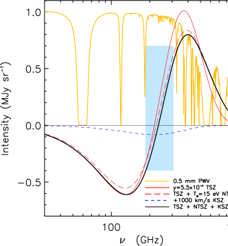
Figure 1.— SZ effect from 30 to $1000\,$GHz. The pure thermal SZ effect with a canonical null at $\nu_{0}=217\,$GHz is shown as a solid red line, the thermal effect including non-thermal corrections as a dashed red line, the kinetic effect for a cluster velocity of $v_{\mathrm{pec}}=+1000\,$km s^-1 as a blue (short) dashed line, and the sum of all three effects — which is the spectrum which would be observed through the cluster — as the solid black line. Also shown are the atmospheric transmittance spectrum for a precipitable water vapor column of $0.5\,$mm at Mauna Kea in yellow (P. Ade 2007, private communication), and the effective bandwidth of Z-Spec on the CSO in the solid blue region. Z-Spec’s spectral range is well matched to span the null in the SZ effect.

At most frequencies, the largest contribution to the sum in Equation (1) is from the thermal SZ (tSZ) effect, given by $\Delta I_{\mathrm{thermal}}=yf(x)\left|dB_{\nu}/dT\right|$. A characteristic property of the tSZ effect is that, because on average CMB photons gain energy from the hot electrons, a decrement in temperature compared to the CMB arises at low frequencies, and an increment arises at high frequencies. The crossover between the increment and decrement occurs at $\nu_{0}=217\,$GHz and is the “null” of the SZ effect.

The relativistic SZ (rSZ) effect $\delta(x,T_{\mathrm{e}})$ in Equation (1) arises because a full description of the scattering properties of the ICM gas requires corrections due to the relativistic velocities of very hot electrons in the ICM. These corrections are typically small in the Rayleigh–Jeans part of the spectrum, but become large near the SZ effect peaks and null: for example, at the maximum of the SZ increment, this correction changes the SZ flux by $18\,$% for a $kT_{\mathrm{e}}=15\,$keV cluster (Wright 1979; Challinor & Lasenby 1998; Itoh et al. 1998; Nozawa et al. 2000). The shift in the position of the null for such a cluster is $\Delta\nu/\nu\approx 5\,$%, which is substantial; more importantly, as the non-thermal corrections depend on $x$, their effect on the spectrum also changes with observing frequency. This means that a sufficiently accurate measurement of the SZ effect spectrum at different frequencies can allow a measurement of the amplitude of the relativistic corrections to the tSZ effect (Hansen et al. 2002, Zemcov et al. 2010).

In contrast, the kinetic SZ (kSZ) effect $k(v_{\mathrm{pec}})$ has the same spectral shape as the CMB but scales according to the line-of-sight peculiar velocity of the cluster. Importantly, the kSZ spectrum does not have an intensity null, but rather is entirely positive or negative depending on the velocity of the cluster. For reasonable cluster velocities given structure formation models — usually $\approx 1000\,$km s^-1 — the ratio of the $217\,$GHz kinetic SZ effect brightness and the peak increment brightness due to the combined thermal and non-thermal effects is $\lesssim 10\,$%. Though faint, such levels can be reached with the current generation of instruments (Benson et al., 2003).

As tSZ effect probes only the pressure of the ICM, the rSZ corrections and kinetic SZ effect allow more detailed studies of the ICM. However, due to degeneracies between the tSZ spectrum and both the rSZ and kSZ spectra, it is often difficult to disentangle all three components, even with multi-band data. This is especially true in the presence of cluster substructure. Though difficult to measure, the rSZ effect can be used to study the temperature of the ICM, especially at the high temperatures that are difficult to constrain with current X-ray facilities, and at high redshifts where X-rays are attenuated by cosmological dimming. For example, Prokhorov et al. (2011) show that a comparison of SZ images at different frequencies can allow measurements of the morphology of the temperatures in ICMs through the changing emission from the rSZ corrections. Although similarly difficult to measure, the kSZ effect can be used to study cosmology by constraining the peculiar velocites of clusters, and to study cluster astrophysics by constraining the velocities of bulk flows within the cluster itself (see (Birkinshaw, 1999) for a comprehensive review). In addition, the kSZ and rSZ signals can be used together to constrain complex temperature and velocity substructures due to merging activity in clusters (Diego et al. 2003; Koch & Jetzer 2004; Prokhorov et al. 2010). In either case spectral information, preferably spanning the null in the SZ effect, is key.

Z-Spec is a multi-channel spectrometer working in the $220\,$GHz atmospheric window with 160 independent spectral channels running from 185 to $305\,$GHz (Bradford et al., 2004). Z-Spec’s spectral range almost ideally spans the SZ effect null and so provides a unique opportunity to measure the transitional frequencies where the tSZ effect passes from a decrement to an increment in surface brightness with high spectral resolution. In principle, such measurements can tightly constrain the position of the SZ null as well as the presence of any foreground or background emission via measurements of line emission. In this paper, we present millimeter (mm)/submillimeter (sub-mm) Z-Spec measurements spanning the SZ null in the massive, SZ-bright galaxy cluster RX J$\,1347.5{-}1145$. Additional Bolocam (Haig et al., 2004) data are used to build a model of the spatial shape of the SZ emission in the cluster, and to help constrain the kSZ corrections in it. The paper is structured as follows: a description of the observations performed is presented in Section 2, and the data analysis procedure is described in Section 3. Sections 4 and 5 present the results and the simulations required to interpret them, and finally a discussion of the implications of this work, respectively.

2. Observations

Both Z-Spec and Bolocam observations are used in this work and are detailed below. Though this paper primarily addresses measurement of the spectral shape of the SZ effect with Z-Spec, a spatial model of the cluster is necessary to interpret the spectral measurement, for which we use the Bolocam maps. Bolocam also adds a lower frequency datum with small uncertainties to the SZ spectrum which is used in Section 4.3.

2.1. Z-Spec Observations

Descriptions of the instrumental design of Z-Spec and the tests used to characterize its performance are described in, e.g., Bradford et al. (2004), Naylor (2008), and Bradford et al. (2009); here we review the details salient to this work. Z-Spec is a grating spectrometer which disperses the input light across a linear array of 160 bolometers. The curved grating operates in a parallel plate waveguide fed by a single-moded feed horn, which is coupled to the telescope via specialized relay optics. As with all grating spectrometers, the spectral range of the instrument is set by the geometry of the input feed, grating, and detector elements; for the Z-Spec configuration discussed in this work, the spectral range is measured as $185\,$GHz $\leq\nu\leq 307\,$GHz. The resolving power of the grating varies across the linear array, providing single-pixel bandwidths of $\Delta\nu=500\,$MHz at the low-frequency end of the range to $\Delta\nu=1200\,$MHz at the high-frequency end with a mean value of $\Delta\nu=750\,$MHz. Measurements of the spectral bandpass of each of the detectors on the ground and measurements of line positions of bright astronomical sources yield an uncertainty on the central bandpass of the detectors less than $200\,$MHz. In order to achieve photon background limited performance, the detectors, grating and input feed horn are housed in a cryostat and the entire assembly is cooled with an adiabatic demagnetization refrigerator to between 60 and $85\,$mK. The detectors, which are designed and fabricated at JPL, have noise equivalent powers of $4\times 10^{-18}\,$W Hz^-1/2 which make them the most sensitive, lowest-background detectors used for astrophysics to date.

Z-Spec has been operating as a PI instrument at the Caltech Sub-millimeter Observatory (CSO) on Mauna Kea, Hawaii since 2007. Z-Spec employs a chop and nod technique to remove the in-band atmospheric emission, which is the largest source of time-correlated noise in the system. Since it is not possible to modulate the spectral response of the instrument, the chopping secondary mirror of the telescope is used to provide on-sky modulation. In general, there is non-negligible SZ emission beyond the virial radius of massive galaxy clusters, typically corresponding to 1–2 Mpc or a few arcminutes at moderate $z$. This means that chopping and nodding using throws designed for point source observations will typically not be large enough to put the telescope beam off the cluster. The presence of this signal in the off-beams in turn attenuates the observed signal since non-zero astronomical flux is differenced from the main observation beam as part of the signal modulation. In order to mitigate this effect, a target which is bright, compact, and does not have sub-mm bright galaxies in the measurement or chopping beams is desirable. RX J$\,1347.5{-}1145$ at $z=0.451$, one of the brightest known X-ray and SZ clusters, fulfills these criteria. The SZ emission in this cluster has been mapped at several frequencies in the past including in the Rayleigh–Jeans regime (e.g., Reese et al. 2002; LaRoque et al. 2006), at the peak of the decrement (e.g., Komatsu et al. 2001; Pointecouteau et al. 2001), and near the peak of the increment (e.g., Komatsu et al. 1999; Zemcov et al. 2007). The bulk SZ emission in this cluster is unusually centrally peaked and bright with a measured $y_{0}\sim 5\times 10^{-4}$ and $kT_{\mathrm{e}}>15.0\,$keV (Bradač et al., 2008); this means that the expected SZ emission will have exceptionally high contrast between the center and chop positions. In addition, two especially SZ-bright regions associated with shocked gas falling into the cluster lie $\sim 10\,$arcsec away from its center (Komatsu et al. 2001; Mason et al. 2010). Compared to other clusters the foreground and background contamination in RX J$\,1347.5{-}1145$ is slight; the maps of Zemcov et al. (2007) show that there is only a single bright (presumably lensed) sub-mm source originally reported by Kitayama et al. (2004) which could contaminate the SZ effect measurement, but this is easily avoided using a suitable chop throw on the sky. Additionally, works like that of Pointecouteau et al. (2001) and Mason et al. (2010) show that while the central cluster galaxy’s ratio flux is large, it is expected to contribute only $1{-}2\,$mJy over the Z-Spec band; this source also can be avoided by a suitable observation strategy.

RX J$\,1347.5{-}1145$ was observed with Z-Spec on the CSO 2012 March 7 through 12, with a total on-target time of 12.1 hr ($=43.6\,$ks). Z-Spec was pointed toward the SZ-bright shock centered at $13^{\mathrm{h}}47^{\mathrm{m}}31^{\mathrm{s}}.4,-11^{\circ}45^{\prime}25^{\prime\prime}$ (J2000). The weather as measured by the atmospheric opacity $\tau_{225\mathrm{GHz}}$ was excellent; $\tau_{225\mathrm{GHz}}$ had a mean of $0.034$ with a standard deviation of $0.014$ over the six nights of observation. Pointing and spectral flat-field observations bracketed the science observations for each night; these were taken using the radio bright sources 3C279 and 3C345 for whose spectral characteristics are well understood. Calibration observations were taken using Mars, the standard Z-Spec calibration source. As discussed in Bradford et al. (2009), the Z-Spec absolute calibration is determined by a combination of planetary observations and the empirically determined relationship between each bolometer’s operating voltage and responsivity. Based on the consistency of these measurements spanning several years of observations, the channel to channel calibration uncertainties are less than 10 % except at the very lowest frequencies where the $186\,$GHz water line is a strong contaminant. Each observation was taken using a chop and nod technique with a throw of $90\,$arcsec and a chop frequency of $f_{0}=1.62\,$Hz; nods occurred with a frequency of $n_{0}=10.44\,$mHz.

2.2. Bolocam Observations

Bolocam is a large format camera at the CSO with 144 detectors, an 8 arcmin diameter field of view (FOV), an observing band centered at 2.1 mm, and a point-spread function with a 58 arcsec full-width at half-maximum (FWHM; Haig et al. 2004). As part of an ongoing program to image the SZ effect in an X-ray-selected sample of massive galaxy clusters, we observed RX J$\,1347.5{-}1145$ with Bolocam from the CSO in 2008 July and 2009 May. The total on-source integration time is $59\,$ks, approximately evenly split between the two observing periods. The central rms of the beam-smoothed Bolocam data is 16 $\mu$K${}_{\textrm{CMB}}$, and the peak decrement of RX J$\,1347.5{-}1145$ is $\simeq 850$ $\mu$K${}_{\textrm{CMB}}$.

The Bolocam observations were made by scanning the CSO in a Lissajous pattern, with an average scan speed of $4\,$arcmin s^-1. All of the data were reduced following the procedures described in detail in Sayers et al. (2011). In particular, atmospheric noise was subtracted by a combination of an FOV-average template and a time stream high pass filter. A pointing model, accurate to 5 arcsec, was created from frequent observations of the nearby bright object $1334{-}127$ following the methods described in Sayers et al. (2009). The flux calibration, in nV/$\mu$K${}_{\textrm{CMB}}$, was determined according to the procedure described in Laurent et al. (2005), based on observations of Neptune, Uranus, and G34.3 using the brightness values determined in Sayers et al. (2012). We estimate the flux calibration to be accurate to $\simeq 5$% (Sayers et al., 2011, 2012). For the analysis presented in this paper, an elliptical isothermal $\beta$ model was fit to the Bolocam data following the procedures described in detail in Sayers et al. (2011); the best-fitting parameters of this model are given in Table 1. The Bolocam map of RX J$\,1347.5{-}1145$ with the Z-Spec chopping pattern overlaid is shown in Figure 2.

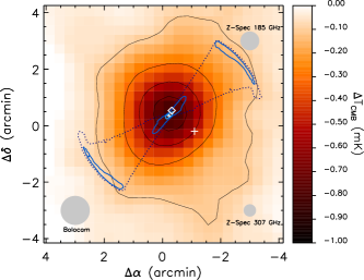
Figure 2.— Bolocam 140 GHz image of RX J$\,1347.5{-}1145$ with the Z-Spec observing scheme superimposed. The Bolocam image has been beam-smoothed to an effective resolution of 82 arcsec, but is otherwise unfiltered (i.e., the effects of noise filtering have been deconvolved). The central rms per beam in the image is 16 $\mu$K${}_{\textrm{CMB}}$. The blue contours show how the Z-Spec observations were performed; the central point is the “on-source” beam while the extended lobes show the effective integration time on the two chop/nod positions. Integrating the chop lobes would yield the same integration time as was spent on the cluster. This figure highlights the traditional difficulty with SZ observations using a chop and nod scheme, which is that it is difficult to chop the beam of the instrument far enough to fall on a region with small SZ amplitude. Given Z-Spec’s 90 arcsec chop throw we naively expect a reduction in the measured SZ amplitude by a factor of $\sim 0.5$. In addition, we have indicated the positions of the central AGN in this cluster with a diamond symbol, and the position of the known sub-mm bright source with a cross. Finally, the angular size of the FWHM of the beams of both Bolocam and the extreme high and low frequencies of Z-Spec are shown as gray circles at the edges of the image.

3. Data Analysis

The standard Z-Spec data analysis pipeline is used to account for instrumental effects, perform the calibration from voltage to astronomical flux, and rectify the chop modulation. In addition, customized data cuts and simulations are required to interpret these data. We describe this data reduction and simulation work in detail in this section.

3.1. Data Reduction

The Z-Spec data reduction pipeline is designed to extract astronomical signals from the measured data time lines which include a variety of instrumental effects as well as statistical noise; a detailed description of this pipeline can be found in Naylor (2008). The basic building blocks of the data analysis are individual data files consisting of 20 nods or $33$ minutes of data; these contain the merged raw time-ordered data (TOD), telescope pointing, chop and nod positions, and general housekeeping data from the telescope.

The first step in the reduction pipeline is to deglitch the TOD which is performed by applying a simple $\sigma$-clip based on statistics calculated from $1000$ sample long windows; all points more than $3\sigma$ from the mean of the time line for each bolometer are masked. These deglitched data are then low pass filtered using a Kaiser window with a pole at $4.5\,$Hz and are down sampled by a factor of three. Since the average of Z-Spec TOD does not reflect the absolute value of the astronomical sky, each raw time line is then mean subtracted to yield zero mean over the full chop/nod cycle in each TOD set.

The data files contain the raw secondary mirror encoder which monitors the position of the chop; this occurs at a predictable rate with a uniform though complex waveform. To simplify the analysis, the chopper data are filtered and down sampled in the same way as for the TOD and an artificial pure tone modulation function phase locked with the chopper signal is generated. An additional complexity is the possible presence of phase shifts between the chopper encoder and the bolometer readout. Calibration observations of bright sources are used to measure and correct the pure tone rectification signal for this phase delay, which are found to be stable over a night of observing. Given the phase delay, the per nod TODs are demodulated using the appropriate pure tone model to yield the signal accounting for the chop pattern, and the power in single half nod (i.e., over the “A” or “B” component of the standard ABBA-style difference) is found. These demodulated averages are then subtracted from one another using the standard ABBA formulation (Zemcov et al., 2003) to yield the measurement for each nod cycle. These averages, which each comprise the average of a $100\,$s long measurement of the spectrum of the sky for each bolometer, are then passed to the next stage of processing.

In order to determine the uncertainty associated with each nod measurement, the white noise level of the time streams is measured. The power spectral density (PSD) of the raw per nod time streams is generated, and a window function defined by $1.4\,$Hz $<f<2.5\,$Hz is generated. This window is designed to sit above the $1/f$ knee in the data and below the second harmonic of $f_{0}$. The noise level in the PSD over this window excluding the points about the first harmonic of $f_{0}$ is calculated and assigned as the uncertainty in the data for that nod. This is repeated for all nods in the data set.

To produce the final sky spectrum, all of the individual nods must be combined. This is performed using a noise-weighted average, where the noise weights are the variance derived from the PSD. Figure 3 shows the spectra measured in each individual nod for the RX J$\,1347.5{-}1145$ observations and the noise-weighted co-addition of the nods. Bolometer 81, monitoring the $232\,$GHz channel, is known to have no optical response and is removed from further analysis. Also plotted in Figure 3 is the measured emissivity of the atmosphere in the Z-Spec band during these observations; the co-added nod spectrum and the atmospheric emissivity are strongly correlated. Investigation of the individual nods shows that in many cases, particularly during periods of large noise, the nods have the shape of the atmospheric emission. This is due to gradients in the overall amplitude of the sky brightness temperature which cause the atmospheric signal to decorrelate on timescales faster than the chop ($f\gtrsim 1\,$ Hz). Though generally below the noise floor per chop cycle, these gradients add constructively over many chop cycles and can cause significant nod cancellation failure. Examination of the individual nod-differenced spectra shows that only a fraction of the nods show structure correlated with the atmospheric emission, which suggests that those spectra showing such structure can be found and masked from the co-addition algorithmically.

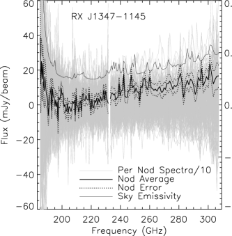
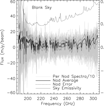
Figure 3.— Raw nod spectra, averages and sky emissivity for the RX J$\,1347.5{-}1145$ (left panel), and blank sky (right panel) fields. Each plot shows the set of raw nod spectra as measured by Z-Spec (gray lines) and the per bolometer variance-weighted mean (black solid lines), and error on the mean (black dashed lines). The raw nod spectra have been scaled by a factor of 10 to allow them to be plotted on the same axis as the mean. Plotted on the same panel scaled to the right hand axis is the mean sky emissivity $\epsilon$ for both targets. The nod averages are strongly correlated with $\epsilon$ for each bolometer, which is evidence that the atmospheric emissivity is varying on short timescales and summing to affect the behavior over a nod cycle.

Z-Spec data are available which allow blind construction of a data masking algorithm. Z-Spec observed a random dark spot on the sky centered at $17^{\mathrm{h}}19^{\mathrm{m}}10^{\mathrm{s}}.3,{+}58^{\circ}55^{\prime}54^{\prime\prime}.2$ on 2011 May 11 and 12 for a total of $6.6\,$hr ($=23.6\,$ks) using the same azimuth chop and nod scheme as were used in the RX J$\,1347.5{-}1145$ observations. Figure 3 also shows the individual nod spectra, noise-weighted average spectrum, and atmospheric emissivity for the blank sky observations. Here, the correlation with the atmospheric emissivity is slightly less pronounced than in the RX J$\,1347.5{-}1145$ observations, though still present. Sayers et al. (2010) present a detailed analysis of the fluctuation properties of the atmosphere from the CSO in a band centered at $268\,$GHz and shows that, though there is a statistical correlation between the atmospheric noise and sky emissivity, the variation in the measured atmospheric stability at a single value of sky emissivity is almost as large as the variation between different sky emissivities. This is thought to arise from night to night variations in the power spectrum of the atmospheric turbulence, along with variations in the height and drift speed of the turbulent layer(s), and is not predictable from models. It is therefore not surprising that, though the sky emissivity is higher in the blank sky data, the nod mis-subtraction is less pronounced since long timescale fluctuations in the sky emissivity do not necessarily track with its absolute level.

The data cutting algorithm we develop is built on the assumption that the continuum sky signal has very little curvature across the Z-Spec band, while the atmosphere has the “U”-shaped spectrum shown in Figure 3. In detail, the algorithm employs the following steps. First, the noise-weighted spectral average of all nods with no cut is generated and the line $\mathbf{y}$ is fit to it; as the simplest model of a continuum astronomical signal the linear model provides a template against which the measured spectra can be compared. Next, for each nod’s spectrum $\mathbf{d}$, the quantity

$$\xi=\sum_{i=1}^{10}|\frac{d_{i}-y_{i}}{\sigma_{i}}|+\sum_{i=150}^{160}|\frac{d_{i}-y_{i}}{\sigma_{i}}|,$$ (2)

is computed, where $\mathbf{\sigma}$ is the uncertainty of the spectrum and $i$ runs over the shortest 10 frequency bins in the first summand and the longest 10 in the second. The $\xi$ statistic is a measure of how much the low- and high-frequency components of the spectra deviate from the linear model, and essentially corresponds to a sum of the number of sigma away from the mean these points lie. The first and last 10 frequency bins are chosen because these are the most sensitive to the water lines bracketing the Z-Spec band and most likely to exhibit failures in the nod modulation; empirically we find that points further inside the band than this do not have much curvature, though at the high-frequency end this is a relatively soft choice. To generate the mask, all nods with $\xi$ greater than some value $\xi_{0}$ are flagged to be cut. The process is then iterated with the average and line fit being generated from the remaining nods and a recomputation of $\xi$ for each nod. The free parameters of this algorithm are the number of iterations to perform and the value of $\xi_{0}$: we empirically find that the blank sky spectrum is consistent with zero when cuts are performed using two iterations of the algorithm and $\xi_{0}=10$, though the result is not strongly sensitive to the choice of $\xi_{0}$ for $\xi_{0}\leq 20$. Figure 4 shows the result of this procedure for the blank sky data, which has a spectrum consistent with zero after the cuts are applied. When the same algorithm is performed on the RX J$\,1347.5{-}1145$ data, the average spectrum shown in the left hand panel of Figure 4 results. This spectrum is now statistically uncorrelated with the sky emissivity.

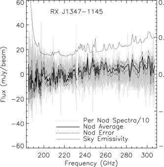
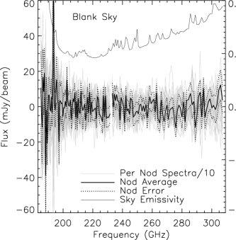
Figure 4.— Nod spectra, averages and sky emissivity for the RX J$\,1347.5{-}1145$ (left panel), and blank sky (right panel) field using only those data passing the data cuts constructed with the algorithm presented in Section 3.1. The data are presented as described in Figure 3. The masking procedure has rejected those nod data with spectra following the sky emission spectrum, leaving a flat spectrum in the case of the blank sky data. When the same algorithm is used on the RX J$\,1347.5{-}1145$ data, the left-hand panel results.

The fraction of data cut using this procedure is $31\,$% for RX J$\,1347.5{-}1145$ and $43\,$% for the blank sky field. In the case of the RX J$\,1347.5{-}1145$ observations for which there are data from six continuous nights, we note that the large proportion of the data cut by the algorithm belong to only three of the observing nights (during which only 27 % of the total data volume was acquired). This matches the expectation that the level of atmospheric fluctuations are similar over timescales of several hours, but can change substantially between nights (Sayers et al., 2010).

It is possible that there is covariance between bolometer time streams in these data, arising from optical or electrical coupling between the detectors, or correlations in the atmospheric emission itself. To check this, we compute the mean bolometer–bolometer covariance matrix using

$$\mathcal{C}=\frac{1}{N_{\mathrm{nod}}-1}\sum_{i=1}^{N_{\mathrm{nod}}}\left(\mathbf{d_{i}}-\mathbf{\bar{d}}\right)\left(\mathbf{d_{i}}-\mathbf{\bar{d}}\right)^{T},$$ (3)

where again $\mathbf{d_{i}}$ is the spectrum of a single nod, $\mathbf{\bar{d}}$ is the average spectrum over all nods, and the summand runs to the number of nods $N_{\mathrm{nod}}$. The matrix $\mathcal{C}$ has been calculated for both the full set and the cut set of RX J$\,1347.5{-}1145$ observations; these are shown in Figure 5. These show that in the full set of nods the covariance matrix is tracing out the structure of the atmosphere; the signature “U” shape of the sky emissivity is visible along the parts of the covariance matrix involving the lowest and highest frequency bins. Applying the data cuts largely removes these correlations to the point that only the three lowest frequency bins remain strongly covariant; these are excluded from further analysis. We take this as good evidence that residual covariance in the nod spectra arising from short-term fluctuations in the sky emissivity is negligible in the cut data set.

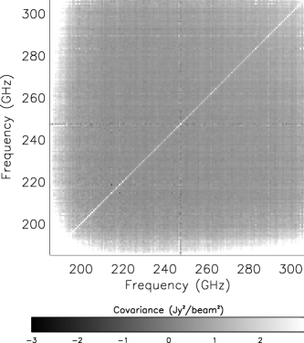
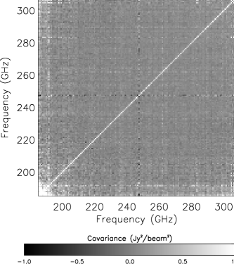
Figure 5.— Covariance matrix of the full and cut nod data. The left-hand panel shows the covariance of the full data set; the characteristic shape of the sky emissivity is present in the bolometer–bolometer covariance, suggesting that the correlations in the individual nod spectra arise from variations in the sky emissivity. The right-hand panel shows the same covariance for the nod set with the data cuts described in Section 3.1 applied; the atmospheric shape has been removed by cutting those nods which have incompletely canceled the variations in the sky emission.

Since neighboring spectral channels are uncorrelated, Z-Spec can measure the absolute level of the spectrum to an accuracy dictated by the (independent) uncertainty in each channel. To estimate the uncertainty in the zero point of the Z-Spec spectra, we compute the band average of a line fit to the blank field spectrum. This procedure yields an estimate of $\pm 0.2\,$mJy on the zero point which can applied to the spectra as a systematic error.

Once these cuts are applied to the data, the resulting spectrum is shown in Figure 6, both in the native Z-Spec binning and as uncertainty-weighted averages in 16 native-element wide bins. Though the native resolution spectrum has low signal-to-noise ratio per measurement, the average shows a clear decrement at low frequencies and increment at high frequencies, which is a signature of the SZ effect; this is investigated further in Section 4.

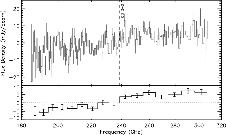
Figure 6.— Measurement of the SZ effect in RX J$\,1347.5{-}1145$ with Z-Spec’s native binning (upper panel) and binned into 16 spectral element wide noise-weighted averages (lower panel). Shown for reference is the position of the CO $J=3\to 2$ line at the redshift of the galaxy cluster; this line would be the brightest available in a dusty sub-mm galaxy, were one coincident with the pointing of the measurement. No individual lines are detected in this spectrum. The lower panel shows that the spectrum of this pointing has a decrement in flux at the lowest wavelengths and an increment at the highest, as would be expected from the SZ effect (see Figure 1).

3.2. Presence of Line Emission

Emission from the SZ effect is purely continuum; if the emission measured with Z-Spec is associated with the SZ effect, no lines will be present in the spectrum. Of course, contamination from sub-mm galaxies along the same line of sight as the cluster could introduce line emission in the Z-Spec spectrum, and further, the presence of such galaxies could contribute (positive) continuum flux to the Z-Spec measurement and bias the result. It is important to search for the presence of line emission in the Z-Spec measurement to show that no contamination from sub-mm galaxies is present in the spectrum.

Current measurements show that two potentially sub-mm bright galaxies reside in this cluster. The central galaxy has been detected by MUSTANG at $90\,$GHz (Mason et al., 2010) but is not detected by SCUBA at $350\,$GHz (Zemcov et al., 2007). In the Z-Spec bands we calculate $S<2\,$mJy across the Z-Spec band for this galaxy (see Section 4.1); this flux will be further diluted by a factor of $\sim 5$ due to its position in the Z-Spec beam. A sub-mm bright galaxy is known exist to the southwest of the cluster center at $13^{\mathrm{h}}47^{\mathrm{m}}27^{\mathrm{s}}.6,-11^{\circ}45^{\prime}54^{\prime\prime}$ (Zemcov et al. 2007; C. D. Dowell 2008, private communication), but this source is far from the both the Z-Spec pointing and chop positions (see Figure 2). We are therefore confident that whatever sub-mm galaxy emission may be present in the Z-Spec spectrum, it is not associated with known, sub-mm bright sources.

No lines are individually detected in the spectrum shown in Figure 6. To search for the presence of faint line emission from sub-mm galaxies, we adopt the algorithm described in Lupu et al. (2010) using the final RX J$\,1347.5{-}1145$ spectrum. The spectrum of RX J$\,1347.5{-}1145$ fails to pass any of the redshift determination criteria described in Lupu et al. (2010). The significance of the redshift determined using this algorithm is $18\,$%, if the noise between channels is uncorrelated under the assumption that multiple lines are present in the spectrum. The spectrum does contain a single $\sim 3\sigma$ feature at $242\,$GHz, however $3\sigma$ deviation in a single bin should arise naturally from statistics given the number of Z-Spec channels.

Of course even in the absence of detected sub-mm sources, the faint, confused sub-mm background will also be present in the Z-Spec beam. A detailed investigation of the effect of the continuum emission from such sources is given in Section 4.2; unfortunately, it is difficult to place limits on the effect of line emission from such sources on this measurement. As a simple check, we compute the histogram of the signal-to-noise ratios of the spectral bins after a quadratic fit is subtracted. As above, a simple quadratic model is a good approximation to the chopped SZ spectral shape over the Z-Spec passband, so is used to remove the continuum emission in the measured spectrum. This resulting histogram should have unity standard deviation if the variation of the data is well described by the instrumental noise estimates; in contrast, if faint lines are present the distribution width will be larger. We fit a Gaussian distribution to the histogram of spectral signal-to-noise ratios and calculate a standard deviation of $1.07\pm 0.07$ for the distribution. This is consistent with the absence of faint lines in the spectrum to the uncertainties of the measurement.

4. Results

The spectrum shown in Figure 6 shows a decrement and increment structure which is indicative of the SZ effect, passing through a null near $220\,$GHz as expected. However, the amplitude of this change is significantly smaller than expected from the previously measured SZ effect (as exemplified in Figure 1). Investigation shows that this reduction is due to the chopping attenuation; Figure 2 shows that the chop throw of $90$ arcsec does not fall off the cluster but rather on a region measured by Bolocam to have $\Delta T_{\mathrm{CMB}}\sim-400\,\mu$K. Since the peak SZ effect in this cluster is measured to have $\Delta T_{\mathrm{CMB}}\sim 850\,\mu$K, we expect a reduction in the measured SZ amplitude of a factor $\sim 2$ from the chop.

Though sensitive to errors in the zero point of the measurement, the frequency of the null in the measured tSZ effect should be independent of its amplitude. As discussed in Section 1, both the rSZ and kSZ corrections can shift the frequency of the tSZ null, and the presence of such a shift in these high spectral resolution Z-Spec measurements would be indicative of the presence of these effects. Though more complex treatments are presented below, in the first instance we use the model which requires the fewest assumptions to determine the shift from the nominal $\nu_{0}$ of the null, which is that the Z-Spec measurements can be approximated by a linear model near the tSZ zero crossing. The null frequency is determined by fitting a line to the Z-Spec measurements for $\nu<260\,$GHz, above which the Z-Spec spectrum measurably deviates from a linear model. The best-fitting model then yields a position for the null whose uncertainties can be calculated from the covariance matrix of the fit using standard error propagation. This calculation using the Z-Spec measurements yields a null frequency of $\nu_{0}=225.8\pm 2.5\,$GHz, which is formally a $3.3\sigma$ detection of the shift in the null of the SZ effect from the canonical tSZ value of $217.5\,$GHz assuming statistical errors only. If the $\pm 0.2\,$mJy systematic uncertainty of the zero point is included an additional uncertainty of $\pm 1.2\,$GHz is accrued, leading to a $3.0\sigma$ measurement of the null shift.

As presented in Itoh et al. (1998), the shift in the null from $217\,$GHz can be approximated by

$$x_{0}=3.830(1+1.1674\theta_{\mathrm{e}}-0.8533\theta_{\mathrm{e}}^{2}),$$ (4)

where $x_{0}$ is the dimensionless null frequency and $\theta_{\mathrm{e}}=k_{\mathrm{B}}T_{\mathrm{e}}/m_{\mathrm{e}}c^{2}$. Under the assumption that $v_{\mathrm{pec}}=0$, the null frequency measured by Z-Spec implies $kT_{\mathrm{e}}=17.1\pm 5.3\,$keV in RX J$\,1347.5{-}1145$; though not the first constraint on cluster temperature from the SZ effect (Hansen et al. 2002; Zemcov et al. 2010), this measurement constitutes the first direct measurement of the temperature of a cluster using the shift in the SZ null frequency. This temperature is consistent with the $kT_{\mathrm{e}}\sim 16\,$keV derived from X-ray data (Section 4.3).

4.1. SZ Likelihood Functions

The simplest way to correct the true amplitude of the SZ effect in RX J$\,1347.5{-}1145$ for the effects of Z-Spec’s chop and demodulation losses is via a simulation which includes a model of the cluster, the observation scheme employed by Z-Spec, and the effects of the data analysis pipeline.

In this work, the cluster SZ shape is modeled using a combination of the SZ effect parameters measured directly by Bolocam for the bulk SZ component and by adopting the model of Mason et al. (2010) for the fine scale component. Since, per resolution element, Z-Spec is essentially a single-pixel narrowband photometer, the spatial model of the cluster cannot be constrained by these Z-Spec data but rather dictates the ratio of the SZ signal in the on- and off-source beams given an SZ effect amplitude (see, for example, Figure 1 of Zemcov et al. 2003 and the associated discussion). In this work, the bulk SZ effect model (reflecting the SZ emission on scales $\gtrsim 1^{\prime}$) is derived via a fit to an elliptical isothermal $\beta$ model using the Bolocam $140\,$GHz map of the cluster; the parameters used in the model are given in Table 1. Uncertainties are given only on the semimajor and semiminor core radii $(\theta_{\mathrm{c,min}},\theta_{\mathrm{c,maj}})$, because these parameters are strongly degenerate with changes in $\beta$ and the uncertainty on them sufficiently encapsulates the uncertainty on the model shape.

The model for fine scale component (for emission on scales $10^{\prime\prime}<\theta<1^{\prime}$) we employ is developed in Mason et al. (2010); since Z-Spec’s beam is large compared to the fine scale components, the details of the fine scale component should not have much effect on the SZ amplitude measured by Z-Spec (this is investigated further in Section 4.2). The rSZ corrections derived by Nozawa et al. (2000) are used to correct the tSZ signal for the effects of the relativistic electron population. As these numerical corrections are only applicable for $kT_{\mathrm{e}}\leq 25\,$keV, all calculations in this work only investigate rSZ corrections up to this temperature.

Table 1Isothermal $\beta$ model parameters for the bulk SZ emission.

Bolocam $\nu_{0}$	$140\,$GHz
$y_{0}^{\mathrm{a}}$ (no rSZ correction)	$5.18\times 10^{-4}$
$\beta^{\mathrm{a}}$	$0.86$
$\theta_{\mathrm{core,min}}$	$37.8\pm 2.5\,$arcsec
$\theta_{\mathrm{core,maj}}$	$46.2\pm 3.1\,$arcsec
P.A.	$-4.6^{\circ}$
Note. a See Section 4 for a detailed discussion of the
uncertainties associated with these parameters.

In a given simulation, the bulk component of the cluster model is given an amplitude corresponding to a particular set of the parameters $y_{0},T_{\mathrm{e},0},$ and $v_{\mathrm{pec,0}}$ reflecting the SZ effect amplitude, ICM electron temperature, and peculiar velocity of the cluster along the line of sight, respectively. The fine scale components are held at a constant $y_{\mathrm{clump}}$ and $T_{\mathrm{e,clump}}$ and are included in the map. Finally, the central radio source in RX J$\,1347.5{-}1145$ is added into the map with a flux given by

$$S_{\mathrm{CS}}(\nu)=S_{\mathrm{CS},0}(\nu/\nu_{0})^{\alpha},$$ (5)

where $S_{\mathrm{CS},0}=60.1^{+49.5}_{-27.1}\,$mJy, $\nu_{0}$ is fixed at $1\,$GHz, and $\alpha=0.77\pm 0.21$; these parameters are determined from an uncertainty-weighted fit to the measurements of Condon et al. (1998), Gitti et al. (2007), Coble et al. (2007), Cohen et al. (2007), and Mason et al. (2010). Due to the frequency at which Z-Spec operates and the offset between the Z-Spec pointing and location of the central cluster source, the details of the source do not have a large effect on the SZ measurement (see Section 4.2). This model map is then smoothed with the Z-Spec optical response function (ORF) at each wavelength; the ORF is modeled by a Gaussian whose width varies according to

$$\mathrm{FWHM}=(a-b/\nu)/\nu,$$ (6)

where the constants $a=8715^{\prime\prime}$ GHz and $b=9312^{\prime\prime}$ GHz² are empirically determined from dedicated beam mapping observations.

These simulated, ORF-convolved maps are then sampled in the same way as Z-Spec sampled the true cluster to generate simulated time-ordered data (sTOD). These sTOD are then propagated through the Z-Spec analysis pipeline starting at the chop demodulation stage using the same settings, data cuts, and filtering as the real data and propagated to an equivalent simulated spectrum. These simulations are noiseless, that is, we do not develop a noise model for the instrument and include random realizations of the instrument noise since we are not estimating the instrumental errors on the spectrum via simulations in this work.

A subtle attenuation factor due to the demodulation model arises from the use of an artificial pure tone to demodulate the chop; this model necessarily picks out only the component of the signal which occurs at the first harmonic of $f_{0}$. This means that, since signal power is mixed to higher harmonics, some fraction of the signal is lost in the $f_{0}$ estimate. With real sky data the absolute calibration and cluster observations are both observed and processed using the same pipeline, so this attenuation is corrected during the calibration step. However, since the simulations are performed in sky-calibrated units, this demodulation attenuation factor is not automatically modeled by the simulations. To account for this, we perform a calibration simulation by populating an empty sky with a single unit flux point source; this is a good model for a Z-Spec calibration observation. This simulated calibration map is then observed in the same way as in a Z-Spec calibration observation. The time streams are then passed through the Z-Spec pipeline in the same way as the cluster simulations to measure the attenuation of the flux due to the demodulation model. The resulting calibration correction factors, which vary over the Z-Spec band from $\sim 50\,$% to $\sim 60\,$% due to the beamwidth at the different Z-Spec resolution bins, are then applied to the simulated spectra to account for the demodulation model attenuation factor. These corrected spectra can then be compared directly to the measurements to compute a likelihood function which varies as a function of the input parameters.

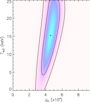
Figure 7.— Likelihood function for the Z-Spec measurement using the cluster model described in Section 4.1 and assuming $v_{\mathrm{pec}}=0$. The color is proportional to the likelihood and the contours show the $68\,$% and $95\,$% confidence regions. The Z-Spec data have a peak likelihood for a model with $y_{0}=4.6\times 10^{-4}$ and $kT_{\mathrm{e}}=15.2\,$keV with a large uncertainty on the bulk cluster temperature.

The most likely cluster parameters are determined using the likelihood function based on this simulation pipeline and the real measurements. The simulator is run with a variety of $y_{0},T_{\mathrm{e,0}}$, and $v_{\mathrm{pec}}$; for each parameter set, the $\chi^{2}$ statistic is computed from the true spectrum measurements and their uncertainties with the simulated spectrum used as the model. The likelihood function is then formed from the grid of $\chi^{2}$ values in the standard way. Figure 7 shows the resulting likelihood in the case where $v_{\mathrm{pec}}=0$, i.e., only $y_{0}$ and $T_{\mathrm{e},0}$ are varied. As shown in the figure, the maximum likelihood occurs at $y_{0}=4.6^{+0.6}_{-0.9}\times 10^{-4}$ and $T_{\mathrm{e},0}=15.2^{+12}_{-7.4}\,$keV, where the uncertainties represent the marginalized $68\,$% confidence intervals of the likelihood. This means that the hypothesis that no rSZ corrections are present is rejected at the $2\sigma$ level, which is less significant than the result from the simpler analysis presented in Section 4.

Figure 8 compares the measured Z-Spec spectrum with the simulated output and model corresponding to the maximum of the likelihood function. This figure highlights the effects of the chop pattern attenuation on the measured signal; for example, at $300\,$GHz the brightness of the measured emission is $6\,$mJy beam^-1, though the simulator allows us to infer that the true SZ brightness should be $13\,$mJy beam^-1 at this frequency in the absence of the chop. Figure 8 highlights a shortcoming of Z-Spec for SZ measurements, which is that the instrument’s effective passband is too narrow to effectively constrain the curvature of the SZ effect spectrum over the band. In terms of the parameters of the spectral model, because $y_{0}$ dictates the amplitude of the signal over the Z-Spec bandpass and the SZ spectrum is close to linear over it, the constraints on this parameter from Z-Spec alone are reasonable given the instrumental sensitivity. However, since both the rSZ and kSZ signals are spectrally broad modifications to the color of the SZ effect, they are much less constrained by even relatively wideband measurements near the SZ null. The case of the rSZ corrections is exemplified in Figure 9: over the Z-Spec bandpass (which covers the entire $220\,$GHz atmospheric window), the rSZ corrections predominantly have the effect of flattening the spectrum of the SZ increment. This means that, in a $\Delta\chi^{2}$ sense, a measurement of $T_{\mathrm{e},0}$ is largely degenerate with a different value of $y_{0}$. Further, because the rSZ corrections are so small, the $\Delta\chi^{2}$ accrued from even large changes in $T_{\mathrm{e},0}$ are not highly constraining. This is what leads to the poor constraints on $T_{\mathrm{e},0}$ in Figure 7; clearly, even high-resolution measurements of the SZ null are not very constraining on the combination of SZ spectral corrections when taken over a relatively narrow bandpass. The situation is even worse in the case of kSZ, which will be discussed in Section 4.3.

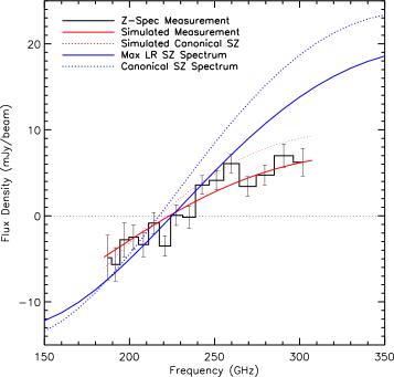
Figure 8.— SZ effect distortions corresponding to the most likely models given the Z-Spec spectral measurement of RX J$\,1347.5{-}1145$. The black line shows the measured Z-Spec points, while the red shows the minimum $\chi^{2}$ model matching the data arising from the input shown by the solid blue line. The difference between the red and blue lines is largely due to the effects of the chop and nod observation strategy and to a lesser extent the varying beams over the Z-Spec bandpass. The dotted blue line shows the canonical tSZ effect spectrum corresponding to the peak in the likelihood function, and dotted blue shows this canonical spectrum propagated through the Z-Spec pipeline; we can differentiate between the canonical and rSZ corrected models using their different amplitudes and shapes.

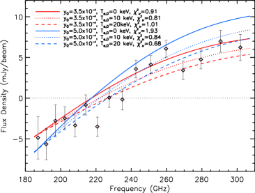
Figure 9.— Difficulty in constraining $T_{\mathrm{e,0}}$ is caused by the combination of Z-Spec’s relatively narrow free spectral range and the small amplitude of the shift in the SZ null from the rSZ effect. This plot shows the binned Z-Spec measurements as the black points, and families of constant $y_{0}$ as red and blue lines. Different values of $T_{\mathrm{e,0}}$ are shown using the line styles as given in the legend, which also lists the $\chi^{2}$ of the fits to the Z-Spec data. As can be seen in this figure, over the Z-Spec bandpass $y_{0}$ dictates the amplitude of the SZ effect, while increasing $T_{\mathrm{e,0}}$ “smooths” the SZ spectrum to shorter $\nu$, shifting the null slightly. This means that the likelihood for a low $y_{0},T_{\mathrm{e,0}}$ combination can be similar to that for a higher $y_{0},T_{\mathrm{e,0}}$ pair. This, in turn, leads to the shape of the likelihood function shown in Figure 7.

4.2. Modeling Uncertainties

The various uncertainties in our model of the cluster emission will lead to uncertainties in the SZ effect parameters measured using the likelihood function; these can be estimated by measuring the variation in the output SZ parameters caused by changes in the model input to the simulator. To do this, the input model parameters are varied within their individual uncertainties and shifts in the best-fitting results are measured. Table 2 lists the model parameters which are varied and the shift each causes from the result $y_{0}=4.6\times 10^{-4},T_{\mathrm{e,0}}=15.2\,$keV presented in Section 4.1.

Table 2Systematic uncertainties in Z-Spec SZ measurement.

Systematic Uncertainty	Parameter Variation	$\delta y_{0}$ ($\times 10^{4}$)	$\delta T_{\mathrm{e},0}$ (keV)
Bulk cluster shape	$\theta_{\mathrm{c}}+\sigma_{\theta}$	$+0.2$	$0$
	$\theta_{\mathrm{c}}-\sigma_{\theta}$	$-0.1$	$+0.8$
Shock region	$1.5\times y_{\mathrm{clump}}$	$-0.2$	$0$
	$0.5\times y_{\mathrm{clump}}$	$+0.2$	$+0.2$
	$0.5\times T_{\mathrm{e,clump}}$	$0$	$+0.8$
	Off	$+0.5$	$-0.2$
Central source	$S_{\mathrm{CS}}+\sigma_{S}$	$-0.1$	$0$
	$S_{\mathrm{CS}}-\sigma_{S}$	$+0.2$	$+0.4$
	Off	$+0.2$	$+1.6$
CIB	Béthermin et al. (2011) model	$0.0$	$\pm 0.1$
Absolute calibration	Abs. Cal. $+10\,$%	$+0.5$	$-0.2$
	Abs. Cal. $-10\,$%	$-0.5$	$+0.2$

To estimate the effect of the uncertainties in the shape of the bulk cluster emission, we vary the isothermal $\beta$ model to the $1\sigma$ uncertainties in the Bolocam measurement of the ICM shape as listed in Table 1. Note that we have fixed $\beta=0.86$ in the ICM model fits to the Bolocam data due to the strong degeneracy between $\beta$ and $\theta_{c}$. The degeneracy is especially strong over the relatively modest spatial dynamic range of both the Bolocam and Z-Spec data, and therefore fixing the value of $\beta$ does not overconstrain the allowed range of ICM profiles.

The parameters of the proposed small-scale shocks in RX J$\,1347.5{-}1145$ are not well understood; it is necessary to investigate the effect of misestimating their amplitudes on the Z-Spec result. The Z-Spec observations are centered on the shock region to the southeast of the cluster center; we therefore expect this shock to have a much greater effect on the Z-Spec results than the smaller shock to the east of the cluster. Because of this we co-vary the two shock parameters by the amounts listed in Table 2 to both $150\,$% and $50\,$% of their nominal $y_{0}$. In addition, the shock temperatures are reduced to $50\,$% of their nominal value of $25\,$keV; since the rSZ corrections of Nozawa et al. (2000) are not applicable at temperatures above this, we do not perform a simulation where $T_{\mathrm{e,0}}$ is larger than its nominal value. Finally, to determine the overall effect of the shock regions, we perform a simulation set where they are not present.

A further test is performed in which the central active galactic nucleus (AGN) in the cluster is both varied by the $1\sigma$ uncertainties on the spectral extrapolation to the Z-Spec band as listed in Section 4.1. Additionally, a test is performed where the AGN source is absent from the cluster model; the results are again listed in Table 2.

The cosmic infrared background (CIB) is potentially a large contaminant to this SZ measurement, though Z-Spec’s large beam size and the steeply falling sub-mm spectra of these sources work in our favor. To determine the effect of the CIB on this measurement, we employ a model for the sub-mm background and simulate Z-Spec spectra which would result from random observations of it (i.e., analogs of the control field discussed in Section 3.1). The CIB model of Béthermin et al. (2011) is used to generate realizations of the sky which have random spectral energy distributions for sources such that each individual Z-Spec resolution element is properly correlated with the others. These maps are then sampled with the Z-Spec chop pattern and the resulting time streams are passed through the Z-Spec analysis pipeline and propagated to spectra as in the previous simulations. Figure 10 shows the resulting spectra from 100 simulations of the sub-mm background. The mean spectrum has a positive bias but a mean of only a few $\mu$Jy beam^-1, and the variance of the spectra has a complex spectral shape but is everywhere $<50\,\mu$Jy beam¹. This is approximately $5\,$% of the amplitudes of either the relativistic corrections or kSZ effect in this cluster; parameter constraints are listed in Table 2.

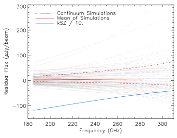
Figure 10.— Simulations of the systematic effect of the faint sub-mm background on these SZ measurements. Simulated maps generated using the Béthermin et al. (2011) CIB model are sampled and propagated through the Z-Spec pipeline, and the resulting spectra for 100 random realizations are shown as dotted gray lines. The mean and single-sided standard deviation of these simulated spectra are shown in red solid and dashed lines. Finally, for comparison, $1/10$ of the amplitude of the best-fitting kSZ spectrum derived in Section 4.3 is plotted in blue. The simulated spectra are asymmetric with respect to zero due to the Z-Spec chopping observation scheme. Though the mean of these 100 simulations is very close to zero, the variation between them can be large, and can involve biases as large as $300\,\mu$Jy if bright sub-mm sources are located in the main chopped beam.

The results of these simulations highlight some interesting behavior in the spectra when Z-Spec observes a random patch of sky. First, as expected, the variance due to the sub-mm background is larger at the shorter wavelengths, about $50\,\mu$Jy beam^-1 with some realizations reaching as much as a few hundred $\mu$Jy beam^-1, compared to the long Z-Spec wavelengths where it is $\sim 10\,\mu$Jy. In addition, due to the chop, the spectra of the confused sub-mm background is asymmetric with respect to zero flux. This is because the chop throw spreads the negative chop lobes over the sky, diluting the effects of bright sub-mm sources, while the on-source position is static on the sky. This means that the rare occasions when a bright sub-mm source falls under the main lobe have large contributions to the variance, while bright sources in the chop lobes do not (see Zemcov et al. 2003 for a detailed discussion). We note that these simulations do not include the effects of lensing, which would amplify background sources near the center of clusters, thereby increasing this bias. Fortunately, in RX J$\,1347.5{-}1145$ we are confident that the sub-mm background is well measured and understood, and that no bright sub-mm sources lie in either the on source or chopped positions (e.g., Zemcov et al. 2007; M. Zemcov et al. in preparation). However, in a hypothetical large survey of clusters searching for spectral corrections with a chopping instrument like Z-Spec, we expect that this asymmetry bias due to the lensing amplification would be among the most important systematic uncertainties.

In addition to overall SZ uncertainties arising from misestimates in the cluster model parameters, we investigate the effect of the uncertainty in the absolute calibration of Z-Spec on the SZ results. Because they can be calibrated from the atmosphere or very bright astronomical sources with known spectra, the relative gains of the spectral channels themselves are well understood and produce a negligible uncertainty on the final SZ results. Specifically, the channel to channel calibration uncertainties are a few percent, leading to a $\sim 0.1\,$% uncertainty on the resulting SZ amplitude. However, there is a $\sim 10\,$% uncertainty in the overall Z-Spec absolute calibration which could affect the scaling of our results to others in the literature. This absolute calibration uncertainty reflects not only the statistical uncertainty of the flux calibration but also the estimated uncertainties arising from the data reduction chain; because of this, we do not vary low level parameters which appear in the reduction pipeline separately as we do for the cluster model parameters. To estimate the effect of the absolute calibration uncertainty, the calibration of the Z-Spec spectrum is varied by $\pm 10\,$% and simulation sets are performed.

As can be seen in Table 2, the largest single uncertainty in the SZ results arises from the presence of the central source. Of course, since it is a well-understood radio source removing it entirely is a very conservative estimate, but this test is illustrative of the effect the AGN source has on the inferred SZ parameters. The bulk cluster shape has the next largest effect on the inferred $T_{\mathrm{e,0}}$, but in the context of the error on the central value of $T_{\mathrm{e,0}}$, which is approximately $\pm 11\,$keV, shifts at the $<1\,$keV level are essentially negligible. The temperature of the shock region has a surprisingly large effect on the SZ effect parameters, but again this is small compared to the overall uncertainty on the ICM temperature. Finally, the absolute calibration has a roughly linear effect on the inferred $y_{0}$ but little effect on $T_{\mathrm{e,0}}$; this is expected since the effect of changes in $y_{0}$ directly tracks scalings in the absolute calibration.

4.3. Constraints on $v_{\mathrm{pec}}$

As a final study, we investigate the effect of the kSZ effect on the Z-Spec measurements and the possibility of constraining it using these data. As shown in Figure 1, the kSZ contribution to the overall SZ spectrum has essentially no curvature over the Z-Spec band; this is highlighted in Figure 11 below. This means that any measurement of kSZ using these high spectral resolution data requires tight constraints on possible systematic errors in the zero point of the Z-Spec spectra. This is further compounded by the degeneracy between kSZ and rSZ if only the shift in the null of the SZ effect is considered. Thus far we have only considered rSZ corrections in this work as rSZ has curvature over the SZ band and its measurement does not rely on precise knowledge of the spectrum zero point alone; the addition of kSZ changes the constraining power of the data entirely.

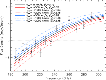
Figure 11.— Effect of kSZ on the total SZ effect spectrum over the Z-Spec band. The black points show the binned Z-Spec measurements and the colored lines families of SZ spectra for positive and negative values of $v_{\mathrm{pec}}$ assuming the best-fitting values of $y_{0}$ and $T_{\mathrm{e},0}$ given in Section 4.1. Different line styles are for different values of $v_{\mathrm{pec}}$, and the $\chi^{2}_{\nu}$ associated with each parameter set is listed in the legend. Including the kSZ effect is degenerate with the addition of a zero point offset error to the measured spectrum and is thus difficult to constrain with such a narrow free spectral range. However, large values of $v_{\mathrm{pec}}$ can be excluded by the Z-Spec measurements as knowledge of the zero point is secure to $\pm 1\,$mJy beam^-1.

To help break these degeneracies and to reduce the range of $\{y_{0},T_{\mathrm{e,0}},v_{\mathrm{pec}}\}$ space over which we need to constrain the SZ spectrum, we rely on ancillary data. The Bolocam measurement of $y_{0}$ is extremely constraining since it is limited by the absolute flux calibration of Bolocam, estimated as $\pm 5\,$% (Sayers et al., 2012). For the canonical tSZ spectrum, this corresponds to $y_{0}=(5.18\pm 0.26)\times 10^{-4}$; because Bolocam’s band is in the SZ decrement, including a non-zero ICM temperature simply increases this according to (Itoh et al., 1998)

$$\frac{y_{0}(T_{\mathrm{e,0}})}{y_{0}}\approx\left(1-\frac{T_{\mathrm{e,0}}}{150\mathrm{keV}}\right)^{-1}.$$ (7)

In addition, $T_{\mathrm{e,0}}$ can be constrained using X-ray measurements of the cluster. We use Chandra observations of the cluster which were carried out using the Advanced CCD Imaging Spectrometer between 2000 and 2003. The data reduction and thermodynamic map creation follow the methods of Million et al. (2010). To determine the likelihood function for $T_{\mathrm{e,0}}$ from these X-ray maps, we smooth both the temperature map and the temperature map varied by the $1\sigma$ temperature error map high and low with the Z-Spec beam. The temperature and its $1\sigma$ limits can then be measured at the point Z-Spec observed. This procedure produces a Gaussian likelihood function in $kT_{\mathrm{e}}$ with mean $16.4\,$keV and standard deviation $1.8\,$keV.

To generate the Z-Spec likelihood function, the Z-Spec simulator is run over the $\{y_{0},T_{\mathrm{e},0}\}$ parameter space with $v_{\mathrm{pec}}$ allowed to vary and using the simplifying assumption $\tau_{\mathrm{e}}\approx y\,m_{\mathrm{e}}c^{2}/kT_{\mathrm{e}}$ (Birkinshaw, 1999). The likelihood space for $\{y_{0},T_{\mathrm{e},0}\}$ for each $v_{\mathrm{pec}}$ is computed in the standard way; $v_{\mathrm{pec}}$ is not tightly constrained in a given simulation.

To constrain $v_{\mathrm{pec}}$, the joint likelihood function of the Z-Spec, Bolocam and X-ray parameter sets is constructed by multiplying the individual likelihoods together. We use two methods to determine the most likely $v_{\mathrm{pec}}$ and its uncertainty. The first is to marginalize over the parameters $y_{0}$ and $T_{\mathrm{e},0}$ in the standard way, and the second is to compute the profile likelihood function by finding the maximum likelihood of the solution $\{y_{0},T_{\mathrm{e},0}\}$ pair for each $v_{\mathrm{pec}}$. These should be close to identical if the likelihood function is well behaved. Figure 12 shows the resulting marginalized and profile likelihood functions for $v_{\mathrm{pec}}$. Since these distributions should be well described by a Gaussian function, we fit Gaussians to determine the maximum likelihood and confidence interval on $v_{\mathrm{pec}}$, leading to an estimate of $v_{\mathrm{pec}}={+}450\pm 800\,$km s^-1 for RX J$\,1347.5{-}1145$ from these combined data sets. The simulations do not include an estimate of the effect of the uncertainty on the absolute offset of the Z-Spec spectrum, which given the uncertainty estimate of $\pm 0.2\,$mJy beam^-1 equates to a $v_{\mathrm{pec}}$ uncertainty of $\pm 110\,$km s^-1. Adding this uncertainty in quadrature with the likelihood function uncertainty leads to a final constraint on the peculiar velocity of RX J$\,1347.5{-}1145$ of ${+}450\pm 810\,$km s^-1. This constraint is significantly better than that measured in single clusters measured by, e.g., SuZIE II (Benson et al., 2003), showing the promise of Z-Spec for this kind of measurement.

Figure 10 shows the kSZ amplitude measured here superimposed on the sub-mm background simulation results discussed in Section 4.2. We note that given the $\sim 1\,$mJy amplitude of the kSZ signal inferred in this cluster, the sub-mm background produces a $\sim 5\,$% systematic uncertainty in the measurement. This is possibly smaller than might be expected, but we note that in this case the chopping strategy employed by Z-Spec works to our advantage, causing the faint, confused sub-mm background to largely cancel. Put another way, the faint CIB imposes a limit on the accuracy to which we can measure the zero point of the measurement using the control field data, which we estimate as $\sim 50\,\mu$Jy beam^-1.

Figure 12.— Joint marginalized and profile likelihood functions for $v_{\mathrm{pec}}$ in RX J$\,1347.5{-}1145$ using Z-Spec, Bolocam, and X-ray data. The likelihood measurements are shown in points, and Gaussian distribution fits to these are lines as shown in the legend. The maximum of the likelihood function yields the most probable $v_{\mathrm{pec}}$ and the width yields the statistical uncertainty on the measurement.

5. Discussion

The results presented in this work represent the first high spectral resolution measurements of the SZ effect near its null at $217\,$GHz. The SZ null position is measured as $\nu_{0}=225.8\pm 2.5\mathrm{(stat.)}\pm 1.2\mathrm{(sys.)}\,$GHz, which differs from the canonical null frequency by $3.0\sigma$. By simulating the response of the instrument to the sky, we measure the best fitting SZ model to be $y_{0}=4.6^{+0.6}_{-0.9}\times 10^{-4},T_{\mathrm{e},0}=15.2^{+12}_{-7.4}\,$keV for $v_{\mathrm{pec}}=0\,$km s^-1. When $v_{\mathrm{pec}}$ is allowed to vary, a most probable value of $v_{\mathrm{pec}}={+}450\pm 810\,$km s^-1 is found. Due to differences in modeling, calibration, and assumptions regarding the necessity of spectral corrections to the SZ effect, it is difficult to directly compare the results derived here to those in the literature. Our use of the Bolocam data mitigates this within our analysis since we have full control over the data which image a large area around the cluster to very low noise levels. As a cautionary note, simply varying the $\beta$ model to values found in the literature and fitting to the Bolocam data used here can lead to changes of $25$% in the inferred $y_{0}$ at $140\,$GHz. The same magnitude of variation in $y_{0}$ from the Z-Spec data assuming different models should be expected. We therefore hesitate to perform an in-depth comparison to previous work in RX J$\,1347.5{-}1145$, over which the $y_{0}$ measured can differ from ours by as much as $\sim 250\,$% (e.g., Benson et al. 2004).

Since the Z-Spec constraints are not limited by systematic errors, it should be possible to reduce the uncertainties of Z-Spec measurements substantially. A simple change would be to increase the integration time, which would reduce the uncertainty as $1/\sqrt{t}$ until the close to the systematic error floor. Furthermore, several inefficiencies arise in these measurements because of the chop and nod cycle used in the observations. First, it would be better to chop and nod at a higher frequency to reduce non-cancellation in the chops from changing atmosphere, particularly on poor weather days where the data cut fraction is large. In addition, a chop waveform closer to a sine wave, or alternatively choosing a demodulation waveform closer to the true chop pattern, would increase the in-band signal. Third, selecting a larger chop throw would decrease the SZ-signal attenuation, thereby increasing the signal strength per integration time. Finally, chopping in constant right ascension rather than constant azimuth would allow careful placement of the chopped beams on faint emission positions. A methodological improvement unrelated to the chop would be to acquire more blank sky data to enable more systematics checks. Together, instituting these changes would dramatically increase Z-Spec’s sensitivity to diffuse SZ emission and reduce the uncertainties on both the rSZ and kSZ measurements. We expect instituting these changes and surveying several clusters with both Z-Spec and Bolocam could lead to $v_{\mathrm{pec}}$ constrains several times better than those found with SuZIE II in single clusters.

While the first measurement of its kind, the Z-Spec results presented here yield much more powerful constraints on the SZ spectral corrections when the Bolocam data are included. The cause of this is simple; over a small spectral range like the one afforded by the $220\,$GHz atmospheric window, the changes in the spectral curvature of the tSZ from the SZ corrections are always small. Furthermore, since rSZ, kSZ, and foreground contamination can all lead to a shift in the null of the SZ effect, it is impossible to unambiguously disentangle their contributions from the SZ null shift alone. For this reason, if the goal were to measure spectral corrections to the SZ effect, it would be preferable to observe at many wavelengths. However, combining measurements from different instruments is difficult due to the various cross-calibration uncertainties which exist: it is better to use a single instrument taking data in several bands at once whose cross-band calibrations are well understood. As a general rule, an $R\sim 5{-}10$ imaging instrument with at least several bands between 15 and $600\,$GHz would be the best choice, as this optimizes the trade-off between bandwidth and spectral resolution over the entire SZ spectrum. The successful SuZIE series of instruments (Holzapfel et al., 1997) are an early example of this approach, as are the MAD (de Petris et al., 2007), OLIMPO (Masi et al., 2008), and the Planck Surveyor (Planck Collaboration et al., 2011). In the near future MUSIC, scheduled to be deployed at the CSO in 2012, will have four bands with $5\lesssim R\lesssim 15$ between 150 and 350 GHz filling a 14 arcmin FOV, which will enable imaging of the SZ spectrum over entire clusters (Maloney et al., 2010). Further in the future, the next generation of ground-based mm/sub-mm telescopes placed at high, dry sites like CCAT will have cameras covering two full octaves from $3\,$mm to $750\,\mu$m over perhaps six bands with $R\sim 10$. An instrument like this would allow a major step forward in SZ effect spectral studies.

References

- Benson et al. (2004) Benson, B. A., Church, S. E., Ade, P. A. R., et al. 2004, ApJ, 617, 829
- Benson et al. (2003) —. 2003, ApJ, 592, 674
- Béthermin et al. (2011) Béthermin, M., Dole, H., Lagache, G., Le Borgne, D., & Penin, A. 2011, A&A, 529, A4
- Birkinshaw (1999) Birkinshaw, M. 1999, Phys. Rep., 310, 97
- Bradač et al. (2008) Bradač, M., Schrabback, T., Erben, T., et al. 2008, ApJ, 681, 187
- Bradford et al. (2004) Bradford, C. M., Ade, P. A. R., Aguirre, J. E., et al. 2004, in Society of Photo-Optical Instrumentation Engineers (SPIE) Conference Series, Vol. 5498, Society of Photo-Optical Instrumentation Engineers (SPIE) Conference Series, ed. C. M. Bradford, P. A. R. Ade, J. E. Aguirre, J. J. Bock, M. Dragovan, L. Duband, L. Earle, J. Glenn, H. Matsuhara, B. J. Naylor, H. T. Nguyen, M. Yun, & J. Zmuidzinas, 257–+
- Bradford et al. (2009) Bradford, C. M., Aguirre, J. E., Aikin, R., et al. 2009, ApJ, 705, 112
- Carlstrom et al. (2002) Carlstrom, J. E., Holder, G. P., & Reese, E. D. 2002, ARA&A, 40, 643
- Challinor & Lasenby (1998) Challinor, A., & Lasenby, A. 1998, ApJ, 499, 1
- Coble et al. (2007) Coble, K., Bonamente, M., Carlstrom, J. E., et al. 2007, AJ, 134, 897
- Cohen et al. (2007) Cohen, A. S., Lane, W. M., Cotton, W. D., et al. 2007, AJ, 134, 1245
- Condon et al. (1998) Condon, J. J., Cotton, W. D., Greisen, E. W., et al. 1998, AJ, 115, 1693
- de Petris et al. (2007) de Petris, M., Lamagna, L., Luzzi, G., et al. 2007, New Astronomy Reviews, 51, 368
- Diego et al. (2003) Diego, J. M., Mazzotta, P., & Silk, J. 2003, ApJ, 597, L1
- Gitti et al. (2007) Gitti, M., Ferrari, C., Domainko, W., Feretti, L., & Schindler, S. 2007, A&A, 470, L25
- Haig et al. (2004) Haig, D. J., Ade, P. A. R., Aguirre, J. E., et al. 2004, in Presented at the Society of Photo-Optical Instrumentation Engineers (SPIE) Conference, Vol. 5498, Society of Photo-Optical Instrumentation Engineers (SPIE) Conference Series, ed. C. M. Bradford, P. A. R. Ade, J. E. Aguirre, J. J. Bock, M. Dragovan, L. Duband, L. Earle, J. Glenn, H. Matsuhara, B. J. Naylor, H. T. Nguyen, M. Yun, & J. Zmuidzinas, 78–94
- Hansen (2004) Hansen, S. H. 2004, New Astronomy, 9, 279
- Hansen et al. (2002) Hansen, S. H., Pastor, S., & Semikoz, D. V. 2002, ApJ, 573, L69
- Holzapfel et al. (1997) Holzapfel, W. L., Wilbanks, T. M., Ade, P. A. R., et al. 1997, ApJ, 479, 17
- Itoh et al. (1998) Itoh, N., Kohyama, Y., & Nozawa, S. 1998, ApJ, 502, 7
- Kitayama et al. (2004) Kitayama, T., Komatsu, E., Ota, N., et al. 2004, PASJ, 56, 17
- Koch & Jetzer (2004) Koch, P. M., & Jetzer, P. 2004, ArXiv e-prints astro-ph/0406461
- Komatsu et al. (1999) Komatsu, E., Kitayama, T., Suto, Y., et al. 1999, ApJ, 516, L1
- Komatsu et al. (2001) Komatsu, E., Matsuo, H., Kitayama, T., et al. 2001, PASJ, 53, 57
- LaRoque et al. (2006) LaRoque, S. J., Bonamente, M., Carlstrom, J. E., et al. 2006, ApJ, 652, 917
- Laurent et al. (2005) Laurent, G. T., Aguirre, J. E., Glenn, J., et al. 2005, ApJ, 623, 742
- Lupu et al. (2010) Lupu, R. E., Scott, K. S., Aguirre, J. E., et al. 2010, ArXiv e-prints 1009.5983
- Maloney et al. (2010) Maloney, P. R., Czakon, N. G., Day, P. K., et al. 2010, in Society of Photo-Optical Instrumentation Engineers (SPIE) Conference Series, Vol. 7741, Society of Photo-Optical Instrumentation Engineers (SPIE) Conference Series, 77410F
- Masi et al. (2008) Masi, S., Battistelli, E., Brienza, D., et al. 2008, Mem. Soc. Astron. Italiana, 79, 887
- Mason et al. (2010) Mason, B. S., Dicker, S. R., Korngut, P. M., et al. 2010, ApJ, 716, 739
- Million et al. (2010) Million, E. T., Werner, N., Simionescu, A., et al. 2010, MNRAS, 407, 2046
- Naylor (2008) Naylor, B. 2008, PhD thesis, California Institute of Technology
- Nozawa et al. (2000) Nozawa, S., Itoh, N., Kawana, Y., & Kohyama, Y. 2000, ApJ, 536, 31
- Planck Collaboration et al. (2011) Planck Collaboration, Ade, P. A. R., Aghanim, N., et al. 2011, A&A, 536, A1
- Pointecouteau et al. (2001) Pointecouteau, E., Giard, M., Benoit, A., et al. 2001, ApJ, 552, 42
- Prokhorov et al. (2011) Prokhorov, D. A., Colafrancesco, S., Akahori, T., et al. 2011, MNRAS, 416, 302
- Prokhorov et al. (2010) Prokhorov, D. A., Dubois, Y., & Nagataki, S. 2010, A&A, 524, A89+
- Reese et al. (2002) Reese, E. D., Carlstrom, J. E., Joy, M., et al. 2002, ApJ, 581, 53
- Sayers et al. (2012) Sayers, J., Czakon, N. G., & Golwala, S. R. 2012, ApJ, 744, 169
- Sayers et al. (2011) Sayers, J., Golwala, S. R., Ameglio, S., & Pierpaoli, E. 2011, ApJ, 728, 39
- Sayers et al. (2009) Sayers, J., Golwala, S. R., Rossinot, P., et al. 2009, ApJ, 690, 1597
- Sayers et al. (2010) Sayers, J., Golwala, S. R., Ade, P. A. R., et al. 2010, ApJ, 708, 1674
- Sunyaev & Zeldovich (1972) Sunyaev, R. A., & Zeldovich, Y. B. 1972, Comments on Astrophysics and Space Physics, 4, 173
- Wright (1979) Wright, E. L. 1979, ApJ, 232, 348
- Zemcov et al. (2007) Zemcov, M., Borys, C., Halpern, M., Mauskopf, P., & Scott, D. 2007, MNRAS, 376, 1073
- Zemcov et al. (2003) Zemcov, M., Halpern, M., Borys, C., et al. 2003, MNRAS, 346, 1179
- Zemcov et al. (2010) Zemcov, M., Rex, M., Rawle, T. D., et al. 2010, A&A, 518, L16+