Bloch-Redfield theory of high-temperature magnetic fluctuations in interacting spin systems

Abstract

We study magnetic fluctuations in a system of interacting spins on a lattice at high temperatures and in the presence of a spatially varying magnetic field. Starting from a microscopic Hamiltonian we derive effective equations of motion for the spins and solve these equations self-consistently. We find that the spin fluctuations can be described by an effective diffusion equation with a diffusion coefficient which strongly depends on the ratio of the magnetic field gradient to the strength of spin-spin interactions. We also extend our studies to account for external noise and find that the relaxation times and the diffusion coefficient are mutually dependent.

I Introduction

Recent advances in magnetic imaging techniques, as well as the development of novel types of electronic devices that utilize electronic spin (rather than charge) as an information carrier, have renewed interest in understanding mechanisms of spin noise and spin relaxation. While conventional experimental methods, such as nuclear or electron spin resonance and related techniques amb ; Schlihter , probe the temporal evolution of spin correlations, they typically do not provide much information on spatial correlations between neighboring spins. On the contrary, the new approaches to spin resonance, such as magnetic resonance force microscopy (MRFM), combine capabilities of the usual magnetic resonance techniques with the sensitivity of atomic force microscopy. That is, one can now observe not only the time (frequency) dependence of spin correlations, but also their spatial dispersion with an atomic-scale resolution. Hence, there is a clear need to develop theoretical tools for the description of such correlations in systems of interest, that is, in systems of interacting spins.

The spatial correlations in interacting spin systems are believed to be controlled by the so-called flip-flop processes. That is, two neighboring interacting spins can exchange magnetization, i.e., the values of their spin components can change by $\pm 1/2$, so that the total spin of the pair is conserved. Such exchange gives rise to the diffusion of spin magnetization, provided the dynamics of the flip-flops is Poissonian anderson . Typical calculations of the effective diffusion constant utilize the method of moments, where the line-width is approximated by a gaussian or lorentzian shapeSchlihter . Such approximations are not very well controlled. More recently several types of cluster/cummulant expansions have been proposed in connection with the problem of decoherence of localized electronic spins caused by the fluctuations of nuclear spins souza ; vitzel ; saikin . In that problem though, the decoherence of electronic spins occurs on a timescale small compared to the typical nuclear timescale, which justifies the use of cluster expansions in the description of fluctuations in the nuclear subsystem.

In this paper we study correlations between spatially separated spins in the opposite, long time regime. Such a regime is specifically relevant to the MRFM technique, which utilizes (micro)mechanical cantilevers with ferromagnetic tips to probe magnetic fluctuations in the underlying samples. We propose an approach based on the Markov approximation, similar to the frequently used Bloch-Redfield approximationSchlihter ; blum in the theory of open quantum systems. That is, we consider all possible pairs $(i,j)$ of interacting spins, while other spins $\neq(i,j)$ are treated as an environment, providing finite line-width for the flip-flop transitions through fluctuating magnetic fields (see Fig. 1 for a cartoon visualisation of these approximations). A self-consistency is then established between the flip-flop rates and the line-width so that our approach can be viewed as a sort of dynamical mean field approximation. We argue that our method is well justified, in particular, in the presence of an external strongly non-uniform magnetic field, which introduces separation between the timescales of the flip-flop rates and the correlation time for the fluctuations of the effective magnetic fields. Note that such non-uniform magnetic fields are intrinsic to the MRFM setups, where field gradients are used to address specific spins located within the so-called resonance layer.

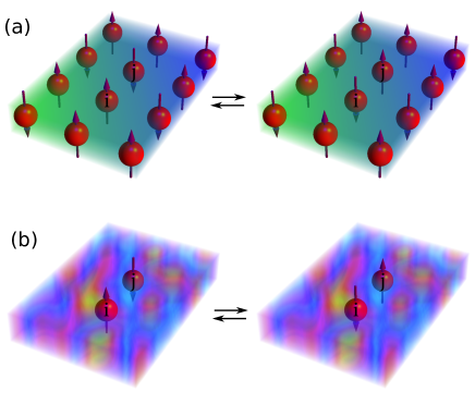
Figure 1: (a) shows a collection of spin-half particles on a rigid lattice in a nonuniform external magnetic field. The quantity of interest in this work is the rate at which spin flip-flops occur. Our model is displayed pictorially in (b), where the neighbouring sites of $i$ and $j$ are replaced by a fluctuating bath. The flip-flop rate is then calculated such that it is consistent with the fluctuations of the bath.

Our paper is organized as follows. In Section II we describe a general formalism that can be utilized to study spin-spin correlations for a broad class of spin Hamiltonians, e.g. Eq. (1). We derive effective equations of motion for the magnetization, e.g. Eq. (12), which has the form of a stochastic master equation. In doing so we use methods developed in connection with studies of diffusion in classical lattice gas models sasha ; kogan as well as in the theory of open quantum systems blum . The equation of motion is supplemented by a self-consistency equation, Eq. (13), which relates the rates in the master equation to the correlation function evaluated from the master equation in terms of the rates. In Section III we look specifically at the Heisenberg model on a cubic lattice in the presence of a spatially non-uniform external magnetic field. We find that the flip-flop rates are strongly suppressed by the field gradient in the limit when the field gradient significantly exceeds the spin-spin interaction constant. In Section IV we study the influence of spin-relaxation processes on spin flip-flops and derive the effective master equation for the magnetization in the presence of external noise sources acting on the spins. Our main result of that section is that, while the field gradient suppresses the flip-flops, the noise may actually enhance these rates; see Eq. (53) and corresponding discussion. Finally, in Section V we discuss the validity of our approximations and summarize the results.

II Model and general solution

We consider a system of spin-half particles on a lattice, interacting with each other according to the following Hamiltonian

$$H\!=\!\sum_{i}B_{i}\sigma^{z}_{i}+\sum_{\langle i,j\rangle}\left[J_{ij}^{\parallel}\sigma_{i}^{z}\sigma_{j}^{z}+2J_{ij}^{\perp}\left(\sigma_{i}^{+}\sigma_{j}^{-}+\sigma_{i}^{-}\sigma_{j}^{+}\right)\right]$$ (1)

where $\sigma^{\pm}_{k}=(\sigma^{x}_{k}\pm i\sigma^{y}_{k})/2$, $k=(k_{x},k_{y},k_{z})$, and $\sigma^{\alpha}_{k}$ are Pauli matrices, $\alpha=x,y,z$. The index $i$ in the first sum runs over all lattice sites, while the notation $\langle i,j\rangle$ in the second sum indicates the summation over all pairs of lattice sites. The external magnetic field $B_{i}$ is assumed to be non-uniform in space. The spin-spin interaction is isotropic when $J^{\parallel}_{ik}=J^{\perp}_{ik}$. The equation of motion for $\sigma^{z}_{i}$ is

$$i\partial_{t}\sigma^{z}_{i}=[\sigma^{z}_{i},H]=4\sum_{{k\neq i}}J^{\perp}_{ik}(\sigma^{+}_{i}\sigma^{-}_{k}-\sigma^{-}_{i}\sigma^{+}_{k}).$$ (2)

In Eq. (2) and in the following we set $\hbar=1$. Next we consider the equation of motion for $\sigma^{+}_{i}\sigma^{-}_{k}$. After a straightforward calculation we obtain

$$i\partial_{t}(\sigma^{+}_{i}\sigma^{-}_{k})= 2\,\delta\!B_{ki}^{\rm eff}\sigma^{+}_{i}\sigma^{-}_{k}+J^{\perp}_{ik}(\sigma^{z}_{i}-\sigma^{z}_{k})$$ (3)

$$+2\!\!\sum_{n\neq\{i,k\}}\left[J^{\perp}_{ni}\sigma^{z}_{i}\sigma^{+}_{n}\sigma^{-}_{k}-J^{\perp}_{nk}\sigma^{z}_{k}\sigma^{+}_{i}\sigma^{-}_{n}\right],$$

where $\delta\!B_{ki}^{\rm eff}$ is the difference between effective magnetic fields at sites $k$ and $i$,

$$\delta\!B_{ki}^{\rm eff}=B_{k}-B_{i}+\sum_{n\neq\{k,i\}}\left[J^{\parallel}_{nk}\sigma_{n}^{z}-J^{\parallel}_{ni}\sigma_{n}^{z}\right].$$ (4)

This difference consists of a constant part;

$$\delta\!B_{ki}=B_{k}-B_{i},$$ (5)

and a part which fluctuates (due to spin flips at nearby lattice sites);

$$\delta\!B_{ki}^{\rm fluct}(t)=\sum_{n\neq\{k,i\}}\left[J^{\parallel}_{nk}\sigma_{n}^{z}-J^{\parallel}_{ni}\sigma_{n}^{z}\right].$$ (6)

The larger the number of individual spins contributing to $\delta\!B_{ki}^{\rm fluct}$, the more rapidly fluctuating this quantity becomes. Hence, for systems with sufficiently long-range interactions or high dimensionality $\delta\!B_{ki}^{\rm fluct}$ fluctuates very rapidly.

From Eq. (3) we see that the expectation value of $\sigma^{+}_{i}\sigma^{-}_{k}$ contains a prefactor

$$\Delta_{ik}(t,s)=e^{2i\int_{s}^{t}dt^{\prime}\,\delta\!B_{ik}^{\rm eff}(t^{\prime})},$$ (7)

related to the Larmor precession of spins around the effective magnetic field at sites $i$ and $k$. The fluctuating component of the effective-magnetic-field [see Eq. (6)] causes the precession frequencies at each site to vary. Moreover, if the effective magnetic fields at sites $i$ and $k$ are large, and the number of spins contributing to the fluctuating component of the field [see Eq. (6)] is much greater than one, then from Eq. (3) [or more specifically, the prefactor shown in Eq. (7)], we would expect the Larmor precession frequency of $\sigma^{+}_{i}\sigma^{-}_{k}$ to be very fast (compared to the dynamics of the individual $\sigma^{z}_{n}$ operators) and fluctuate rapidly. Following this logic, we see that the summation of terms $\sigma_{n}^{+}\sigma_{k}^{-}$ and $\sigma_{i}^{+}\sigma_{n}^{-}$ in Eq. (3) is essentially a summation over a rapidly fluctuating object, and will statistically self-average to zero (provided a sufficiently large number of spins contribute to $\delta\!B_{ki}^{\rm fluct}$).

A similar approximation is very common in the theory of open quantum systems, where it is known as the secular or Bloch-Redfield approximation blum . As in the case of open quantum systems it relies on the assumption that the off-diagonal elements of a system’s density matrix $\rho$ are small either due to large splittings between the adjacent energy levels or due to rapid fluctuations from the heat bath. In the present case the fields $\delta\!B_{ki}^{\rm fluct}(t)$, play the role of the heat bath operators and must treated self-consistently, to which we now focus our attention.

By integrating Eq. (3) (with the summation on the right-hand-side neglected) we obtain

$$\sigma^{+}_{i}\sigma^{-}_{k}(t)\simeq-iJ^{\perp}_{ik}\int_{0}^{t}ds\Delta_{ik}(t,s)[\sigma^{z}_{i}(s)-\sigma^{z}_{k}(s)]$$ (8)

$$+\Delta_{ik}(t,0){c_{ik}},$$

where the last term is due to the initial condition of the operator $c_{ik}=\sigma^{+}_{i}\sigma^{-}_{k}(t=0)$. In the high temperature limit the system is disordered and therefore it is natural to assume that the expectation value of $\sigma^{+}_{i}\sigma^{-}_{k}$ is random, with $\langle\langle\sigma^{+}_{i}\sigma^{-}_{k}\rangle\rangle=0$ and $\langle\langle\sigma^{+}_{i}\sigma^{-}_{k}\sigma^{+}_{i^{\prime}}\sigma^{-}_{k^{\prime}}\rangle\rangle=(1/4)\delta_{ik^{\prime}}\delta_{ki^{\prime}}$, provided $i\neq k$ and $i^{\prime}\neq k^{\prime}$. Here the double bracket stands for averaging over the ensemble of density matrices of the system as well as over a particular realization of the density matrix (set by a particular choice of the initial condition), i.e., $\langle\sigma^{+}_{i}\sigma^{-}_{k}\rangle={\rm Tr}(\sigma^{+}_{i}\sigma^{-}_{k}\rho)$ and $\langle\langle\sigma^{+}_{i}\sigma^{-}_{k}\rangle\rangle=\langle{\rm Tr}(\sigma^{+}_{i}\sigma^{-}_{k}\rho)\rangle_{\rho}$, etc.

We wish to substitute Eq. (8) into Eq. (2) to obtain a closed form equation for $\sigma^{z}_{i}(t)$. This can be significantly simplified if we replace the rapidly fluctuating quantity, $\Delta_{ik}(t,s)$, in the integrand in Eq. (8) by its average value. This approximation is in a perfect agreement with our assumption regarding the separation between time scales for the dynamics of the local fluctuating magnetic field at site $i$, and components of the individual spin at site $i$. We make the assumption that, by virtue of the central limit theorem, the random variable $\delta\!B_{ik}^{\rm eff}$ is Gaussian;

$$\langle\Delta_{ik}(t,s)\rangle =e^{2i(B_{i}-B_{k})(t-s)}e^{-2\int_{s}^{t}\int_{s}^{t}K_{ik}(\tau_{1}-\tau_{2})d\tau_{1}d\tau_{2}}$$

$$=e^{2i(B_{i}-B_{k})(t-s)}e^{-4\int_{0}^{|t-s|}K_{ik}(\mu)\left(|t-s|-\mu\right)d\mu}$$ (9)

where

$$K_{ik}(\tau_{1}-\tau_{2})=\langle\delta\!B_{ik}^{\rm fluct}(\tau_{1})\delta\!B_{ik}^{\rm fluct}(\tau_{2})\rangle$$ (10)

is the autocorrelation function of the fluctuating component of the magnetic field gradient between sites $i$ and $k$. Moreover, since Eq. (9) (as a function of $|t-s|$) decays much faster than the evolution of $[\sigma^{z}_{i}(s)-\sigma^{z}_{k}(s)]$, we can employ the Markov approximation, and set $s=t$ which removes the latter term from the integral in Eq. (8) to give

$$\sigma^{+}_{i}\sigma^{-}_{k}(t)\simeq-iJ^{\perp}_{ik}\int_{0}^{t}ds\langle\Delta_{ik}(t,s)\rangle[\sigma^{z}_{i}(t)-\sigma^{z}_{k}(t)]$$ (11)

$$+\Delta_{ik}(t,0){c_{ik}}.$$

Now that we have a formal solution for $\sigma^{+}_{i}\sigma^{-}_{k}(t)$ it is prudent to substitute the expression back into the sum in Eq. (3) which was originally ignored in deriving Eq. (11). In doing so we wish to find an inequality which quantitatively ensures the summation term is small compared to all other terms in Eq. (3). The details of this calculation are straightforward (see Section V for further discussion) and one finds $J_{ik}\ll\Gamma_{ik}$ (where $\Gamma_{ik}$ is the rate at which flip-flops occur and is calculated below) is a sufficient condition to ensure the summation in Eq. (3) remains small.

We now substitute Eq. (11) into Eq. (2), to give

$$\partial_{t}\langle\sigma_{k}^{z}(t)\rangle= \sum_{j\neq k}\Gamma_{jk}\left[\langle\sigma_{j}^{z}(t)\rangle-\langle\sigma_{k}^{z}(t)\rangle\right]+\xi_{k}(t).$$ (12)

The averages in Eq. (12) are taken with respect to a particular realization of the systems density matrix, but not over the ensemble of the density matrices. The coefficient, $\Gamma_{jk}$, represents a rate at which spin flip-flops occur between sites $j$ and $k$ (these can only occur when sites $j$ and $k$ have opposite spin). The expression for this rate is given by

$$\Gamma_{jk}= 4(J_{jk}^{\perp})^{2}\int_{-\infty}^{\infty}\exp\!\!\Bigg{[}2i\delta\!B_{jk}s-$$

$$\qquad\left.4\int_{0}^{|s|}K_{kj}(\mu)\left(|s|-\mu\right)d\mu\right]ds,$$ (13)

where we have used the quickly-decaying property of $\langle\Delta_{ik}(t,s)\rangle$ to extend the upper and lower limits of the integral to $\pm\infty$. The final term in Eq. (12) represents the uncertainty with respect to the choice of the initial conditions of the system, and is given by

$${\xi_{k}(t)=4i\sum_{j\neq k}J_{jk}^{\perp}\left[c_{jk}\Delta_{kj}(0,t)-c_{kj}\Delta_{jk}(0,t)\right].}$$ (14)

Averaging over $\xi_{i}(t)$ corresponds to averaging over an ensemble of different density matrices (each density matrix being distinguished by a unique initial condition). Noting that $\langle\Delta_{ik}(0,t)\Delta_{ki}(0,t^{\prime})\rangle=\langle\Delta_{ki}(t^{\prime},t)\rangle$, and since $\Delta_{ik}(t^{\prime},t)$ is a rapidly fluctuating function of $t-t^{\prime}$, we can make the approximation;

$$\langle\xi_{i}(t)\xi_{j}(t^{\prime})\rangle=2\delta(t-t^{\prime})\left(-\Gamma_{jk}+\delta_{jk}\sum_{m\neq k}\Gamma_{mk}\right).$$ (15)

Together, Eqs. (12) and (15) obviously describe Poissonian dynamics of a coupled two-state system. Indeed, we could have obtained the same result if we had postulated that the dynamics of a given spin (say, at site $i$) is controlled by its flipping rates $-\sum_{k}\tilde{\Gamma}_{ik}\sigma_{i}(1-\sigma_{k})$ and $\sum_{k}\tilde{\Gamma}_{ki}\sigma_{k}(1-\sigma_{i})$, where $\tilde{\Gamma}_{ik}=\Gamma_{ik}+\eta_{ik}$, with $\Gamma_{ik}$ and $\eta_{ik}$ being the constant and fluctuating parts of the rate respectively. In this case $\xi_{i}=\sum_{k}(\eta_{ik}-\eta_{ki})$, c.f. Eq. (14). Note that one can derive Eq. (13) for the rates $\Gamma_{ik}$ within a straightforward perturbative calculation, as shown in Appendix A. There, we calculate the probability of a flip-flop for a pair of spins in the presence of an external fluctuating field (along the $z$-direction). In the current section, we have simply assumed that this fluctuating external field has been created by the neighbouring spins coupled to this pair (see Appendix A for details).

Equations (12) and (15) constitute a closed system of equations, which allows one to evaluate the correlation functions $\langle\sigma^{z}_{i}(t)\sigma^{z}_{k}(t^{\prime})\rangle$. For an arbitrary choice of spin-spin interaction constants $J^{\parallel}_{ik}$ and $J^{\perp}_{ik}$ and external fields $B_{i}$, the rates $\Gamma_{ik}$ in Eqs. (12) and (15), though formally unkown, are expressed in terms of these correlation functions $\langle\sigma^{z}_{i}(t)\sigma^{z}_{k}(t^{\prime})\rangle$ [see Eqs. (13), (10), and (6)]. By evaluating these correlation functions in terms of $\Gamma_{ik}$, one obtains a closed set of equations which one must solve self consistently for $\Gamma_{ik}$. This provides a way of solving for both the rates, $\Gamma_{ik}$ and the correlation functions, $\langle\sigma^{z}_{i}(t)\sigma^{z}_{k}(t^{\prime})\rangle$ for an arbitrary choice of interaction constants; $J^{\parallel}_{ik}$, $J^{\perp}_{ik}$ and external fields; $B_{i}$.

In the next section we will evaluate the $\Gamma_{ik}$ and $\langle\sigma^{z}_{i}(t)\sigma^{z}_{k}(t^{\prime})\rangle$ for a simple choice of coupling constants given by the three dimensional, cubic, Heisenberg model with nearest-neighbor interactions.

Before proceeding to this task we note that in the limit of large field gradient $|B_{i}-B_{k}|\gg J^{\parallel}_{ik}$, the integrand of Eq. (13) rapidly oscillates and therefore the value of the integral decreases with the growth of $|B_{i}-B_{k}|$. In the limit of vanishing rate $\langle\sigma^{z}_{i}(t)\sigma^{z}_{k}(t^{\prime})\rangle\simeq\delta_{ik}$, we find

$$K_{ik}(t-t^{\prime})\simeq\kappa_{ik}=\sum_{m\neq\{i,k\}}(J_{mk}^{\parallel}-J_{mi}^{\parallel})^{2}.$$

Evaluating then, the Gaussian integral in Eq. (13) we obtain

$$\Gamma_{ik}\simeq\frac{4\pi^{1/2}(J^{\perp}_{ik})^{2}}{\sqrt{2\kappa_{ik}}}\exp{\!\left[-\frac{\delta\!B_{ik}^{2}}{2\kappa_{ik}}\right]}.$$ (16)

Thus we predict the rate at which flip-flops occur, and therefore the rate at which spin diffusion occurs, is very small for $|B_{i}-B_{k}|\gg J^{\parallel}_{ik}$.

III Example: Heisenberg model

We now consider a particular example; the Heisenberg model on a cubic lattice with an external spatially varying magnetic field. The Hamiltonian of the system can be cast in the form

$$H=\sum_{i}B({\bf r}_{i})\sigma^{z}_{{\bf r}_{i}}+J\sum_{i,\nu,\alpha}\sigma^{\alpha}_{{\bf r}_{i}}\,\sigma^{\alpha}_{{\bf r}_{i}+{\bf e}_{\nu}}.$$ (17)

where $i=(i_{x},i_{y},i_{z})$, ${\bf r}_{i}=i_{x}a{\hat{\bf x}}+i_{y}a{\hat{\bf y}}+i_{z}a{\hat{\bf z}}$ ($a$ being the lattice spacing), $\nu=1,...,6$ enumerates the unit vectors which point to the nearest neighbors: ${\bf e}_{1(2)}=\pm\hat{{\bf x}}$, ${\bf e}_{3(4)}=\pm\hat{{\bf y}}$ and ${\bf e}_{5(6)}=\pm\hat{{\bf z}}$, and finally $\alpha=x,y,z$. We also assume that the external field varies linearly in space, $B({\bf r})=b_{0}{\bf r}\cdot{\bf g}$ where ${\bf g}$ is a unit vector which points in the direction of variation. The Hamiltonian (17) obviously belongs to the class of Hamiltonians defined in Eq. (1).

The equation of motion for $\sigma^{z}_{{\bf r}_{i}}$ is given by Eq. (12), which, for the Hamiltonian in Eq. (17) reads

$$\partial_{t}\langle\sigma^{z}_{{\bf r}_{i}}\rangle=\sum_{\nu}\Gamma_{\bf{e}_{\nu}}\left[\langle\sigma^{z}_{{\bf r}_{i}+{\bf e}_{\nu}}\rangle-\langle\sigma^{z}_{{\bf r}_{i}}\rangle\right]+\xi_{{\bf r}_{i}}(t)$$ (18)

and the noise $\xi_{{\bf r}_{i}}(t)$ is correlated according to Eq. (15), which becomes

$$\langle\xi_{{\bf r}_{i}}(t)\xi_{{\bf r}_{j}}(t^{\prime})\rangle=2\delta(t-t^{\prime})\sum_{\nu}\Gamma_{\bf{e}_{\nu}}(\delta_{{\bf r}_{i}\,{\bf r}_{j}}-\delta_{{\bf r}_{i}+{\bf e}_{\nu}\,{\bf r}_{j}}).$$ (19)

Eqs. (18) and (19) can be readily diagonalized by a Fourier transform method. Writing

$$\sigma^{z}_{{\bf r}_{i}}(t)=\int_{-\infty}^{\infty}\frac{dt}{2\pi}\int_{-\pi/a}^{\pi/a}\frac{d^{3}{\bf k}}{(2\pi)^{3}}{\tilde{\sigma}}^{z}({\bf k},\omega)e^{i{\bf r}_{i}{\bf k}+i\omega t},$$ (20)

where the ${\bf k}$-integral is taken over the first Brillouin zone, (a cube with an edge $2\pi/a$), we obtain from Eq. (18) that

$$\langle|{\tilde{\sigma}}^{z}({\bf k},\omega)|^{2}\rangle=\frac{\langle|{\tilde{\xi}}({\bf k},\omega)|^{2}\rangle}{\omega^{2}+\{\sum_{\nu}\Gamma_{\bf{e}_{\nu}}\left[1-\cos{(a\,{\bf e}_{\nu}{\bf k})}\right]\}^{2}},$$ (21)

with $i=x,y,z$ and ${\tilde{\xi}}({\bf k},\omega)$ being the Fourier transform of $\xi_{{\bf r}_{i}}(t)$, defined similarly to Eq. (20). From Eq. (19)

$$\langle|{\tilde{\xi}}({\bf k},\omega)|^{2}\rangle=2\sum_{\nu}\Gamma_{\bf{e}_{\nu}}\left[1-\cos{(a\,{\bf e}_{\nu}{\bf k})}\right],$$ (22)

and taking the inverse Fourier transform of Eq. (22), we obtain

$$\langle\sigma^{z}_{{\bf r}_{i}}(t)\sigma^{z}_{{\bf r}_{i^{\prime}}}(0)\rangle=\, e^{-t\sum_{\nu}\Gamma_{\bf{e}_{\nu}}}\times$$

$$\qquad I_{n_{x}}(2\Gamma_{{\bf e}_{1}}t)I_{n_{y}}(2\Gamma_{{\bf e}_{3}}t)I_{n_{z}}(2\Gamma_{{\bf e}_{5}}t),$$ (23)

where $I_{n}(z)$ is the modified Bessel function of complex argument grad and $n_{x}=|i_{x}-i_{x}^{\prime}|$, etc. At sufficiently large distances (and times) Eq. (23) describes (anisotropic) diffusion with diffusion constants $D_{\nu\nu}\sim\Gamma_{\bf{e}_{\nu}}a^{2}$.

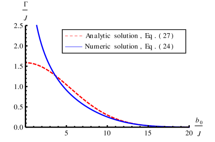
Figure 2: Numerical solution of the integral Eq. (24), showing the rate $\Gamma$ as a function of magnetic field gradient $b_{0}$.

The rates $\Gamma_{\bf{e}_{\nu}}$ are yet to be determined. They can be found from Eq. (13). Note that while for arbitrary direction of the field gradient ${\bf g}$ the rates $\Gamma_{\bf{e}_{\nu}}$, $\Gamma_{\bf{e}_{\nu^{\prime}}}$ differ from each other, they are equal ($\Gamma_{\bf{e}_{\nu}}\equiv\Gamma$) for ${\bf g}={\bf g}_{0}=(1/\sqrt{3})({\hat{\bf x}}+{\hat{\bf y}}+{\hat{\bf z}})$, i.e., when the field gradient points along the main diagonal of the cube formed by the unit vectors $\hat{{\bf x}}$, $\hat{{\bf y}}$ and $\hat{{\bf z}}$. In this case Eq. (15) reduces to

$$\Gamma=4J^{2}\int_{-\infty}^{\infty}ds\,e^{2ib_{0}s/\sqrt{3}}e^{-4\int_{0}^{|s|}d\mu K(\mu)\left(|s|-\mu\right)},$$ (24)

where $K(\mu)$ is the correlation function of Eq. (10), which is now independent of the indices $i$ and $k$, due to our convenient choice of magnetic field gradient direction ${\bf g}$, which makes the diffusion process isotropic. $K(\mu)$ can be easily expressed in terms of $\langle\sigma^{z}_{{\bf r}_{i}}({\mu})\sigma^{z}_{{\bf r}_{j}}(0)\rangle$:

$$K({\mu})=\, \frac{1}{2}J^{2}\left(\sum_{\nu\neq 1}\sum_{\nu^{\prime}\neq 1}\langle\sigma^{z}_{{\bf e}_{\nu}}({\mu})\sigma^{z}_{{\bf e}_{\nu^{\prime}}}(0)\rangle\right.$$

$$\left.-\sum_{\nu\neq 1}\sum_{\nu^{\prime}\neq 2}\langle\sigma^{z}_{{\bf e}_{\nu}}({\mu})\sigma^{z}_{{\bf e}_{1}+{\bf e}_{\nu^{\prime}}}(0)\rangle\right),$$ (25)

where we have chosen to calculate $K$ between sites ${\bf r}_{i}=(0,0,0)$ and ${\bf r}_{j}={\bf e}_{1}$ (and then relied on the isoptropy of all directions in the lattice). Using Eq. (23) we obtain $K(\mu)=\frac{1}{2}J^{2}e^{-6\Gamma\mu}f(2\Gamma\mu)$, where

$$f(x)= 5I_{0}^{3}(x)+16I_{0}(x)I_{1}^{2}(x)+4I_{0}^{2}(x)I_{2}(x)$$

$$-4I_{0}^{2}(x)I_{1}(x)-8I_{1}^{3}(x)-12I_{0}(x)I_{1}(x)I_{2}(x)$$

$$-I_{0}^{2}(x)I_{3}(x).$$ (26)

Substituting this new found expression for $K(\mu)$ into Eq. (24) we obtain an integral equation for $\Gamma$. One can solve this integral equation numerically to find $\Gamma/J$ as a function of $b_{0}/J$ (see Appendix B), the results are shown in Fig. 2. For $b_{0}/J\gg 1$ the value of $\Gamma$ is consistent with Eq. (16), which for the present case reduces to

$${\Gamma\simeq 4J\sqrt{\frac{\pi}{20}}e^{-b_{0}^{2}/(60J^{2})}.}$$ (27)

The analytic solution is also shown in Fig 2 for comparison. We find the analytic and numerical solutions are equal beyond $b_{0}\gtrsim 10J$.

IV Influence of relaxation processes

In this section we consider the influence of external noise on the spin-spin correlation function. We consider a model described by the Hamiltonian

$${\tilde{H}}=H+\sum_{i,\alpha}\eta^{\alpha}_{i}(t)\,\sigma^{\alpha}_{i},$$ (28)

where $H$ is given by Eq. (1) and $\eta^{\alpha}_{i}(t)$ is a fluctuating magnetic field. The index $i$ runs over lattice sites, and $\alpha=x,y,z$. In reality such a field may arise due to phonons (for instance in semiconductors) or conduction electrons (for instance in metals). We will assume that $\langle\eta^{\alpha}_{i}(t)\eta^{\beta}_{j}(t^{\prime})\rangle=\delta_{\alpha\beta}\,\delta_{ij}\,\Lambda(t-t^{\prime})$, where $\Lambda(t)$ is some even function which decays to zero over some time scale.

We follow a similar procedure as in Section II. By calculating commutation relations, we find;

$$i\partial_{t}\sigma_{k}^{z}=4\sum_{j\neq k}J_{jk}^{\perp}\left(\sigma_{k}^{+}\sigma_{j}^{-}-\sigma_{j}^{+}\sigma_{k}^{-}\right)+4\left(\eta_{k}^{-}\sigma_{k}^{+}-\eta_{k}^{+}\sigma_{k}^{-}\right)$$ (29)

where $\eta_{k}^{\pm}=\frac{1}{2}\left(\eta_{k}^{x}\pm i\eta_{k}^{y}\right)$.

$$i\partial_{t}\sigma_{k}^{+}=-2B_{k}^{\rm eff}\sigma_{k}^{+}+2\eta_{k}^{+}\sigma_{k}^{z}+2\sum_{j\neq k}J_{jk}^{\perp}\sigma_{k}^{z}\sigma_{j}^{+}$$ (30)

where $B_{k}^{\rm eff}=B_{k}+\sum_{j\neq k}J^{\parallel}_{jk}\sigma_{j}^{z}+\eta_{k}^{z}$ is the effective magnetic field at site $k$. Also

$$i\partial_{t}\sigma_{k}^{-}=2B_{k}^{\rm eff}\sigma_{k}^{-}-2\eta_{k}^{-}\sigma_{k}^{z}-2\sum_{j\neq k}J_{jk}^{\perp}\sigma_{k}^{z}\sigma_{j}^{-}.$$ (31)

Finally,

$$i\partial_{t}\left(\sigma_{j}^{+}\sigma_{k}^{-}\right)=\, 2\Delta\!B_{kj}^{\rm eff}\sigma_{j}^{+}\sigma_{k}^{-}+J_{jk}^{\perp}\left(\sigma_{j}^{z}-\sigma_{k}^{z}\right)+$$

$$2\left[\eta_{j}^{+}\sigma_{j}^{z}\sigma_{k}^{-}-\eta_{k}^{-}\sigma_{j}^{+}\sigma_{k}^{z}\right]+$$

$$2\sum_{i\neq\{j,k\}}\left[J_{ij}^{\perp}\sigma_{j}^{z}\sigma_{i}^{+}\sigma_{k}^{-}-J_{ik}^{\perp}\sigma_{k}^{z}\sigma_{j}^{+}\sigma_{i}^{-}\right]$$ (32)

where $\Delta\!B_{kj}^{\rm eff}=\delta\!B_{kj}^{\rm eff}+\eta_{k}^{z}-\eta_{j}^{z}$, and $j\neq k$. Analagous to Eqs. (5) and (6) of Section II, $\Delta\!B_{kj}^{\rm eff}$ consists of a constant part, given by ${\delta\!B_{kj}}$ [see Eq. (5)], and a fluctuating part, which is now given by

$$\Delta\!B_{kj}^{\rm fluct}(t)=\delta\!B_{kj}^{\rm fluct}(t)+\eta_{k}^{z}(t)-\eta_{j}^{z}(t),$$ (33)

compared with Eq. (6). We wish to integrate Eqs. (30), (31), and (32), and thereby find a closed form for the time evolution of $\sigma_{k}^{z}$ from Eq. (29).

We start with Eqs. (30), and (31) and apply the same logic as in Section II regarding the self-averaging nature of the summations (due to a fluctuating Larmor precession frequency). What is left can easily be integrated to give

$$\sigma_{k}^{\pm}(t)=\, \mp 2i\int_{0}^{t}\left[e^{\pm 2i\int_{s}^{t}B_{k}^{\rm eff}(\tau)d\tau}\eta_{k}^{\pm}(s)\sigma_{k}^{z}(s)\right]ds+$$

$$\quad c_{k}^{\pm}e^{\pm 2i\int_{0}^{t}B_{k}^{\rm eff}(\tau)d\tau},$$ (34)

where $c_{k}^{\pm}=\sigma_{k}^{\pm}({t=}0)$ gives the contribution from the initial conditions. Looking now at Eq. (32), and ignoring the summation term, we find

$$\sigma_{j}^{+}\sigma_{k}^{-}(t)\!=\!-i\int_{0}^{t}\Delta_{jk}^{\prime}(s,t)\Bigg{\{}\left[J_{jk}^{\perp}+2\eta_{j}^{+}(s)\sigma_{k}^{-}(s)\right]\sigma_{j}^{z}(s)-$$

$$\!\!\left[J_{jk}^{\perp}+2\eta_{k}^{-}(s)\sigma_{j}^{+}(s)\right]\sigma_{k}^{z}(s)\Bigg{\}}ds+c_{jk}\Delta_{kj}(0,t)$$ (35)

where $\Delta_{jk}^{\prime}(s,t)=e^{2i\int_{s}^{t}\!\Delta\!B_{jk}^{\rm eff}(\tau)d\tau}$, and $c_{jk}=\sigma_{j}^{+}\sigma_{k}^{-}(0)$ is the initial condition. Substituting Eq. (35) into Eq. (29), we find that the terms $2\eta_{j}^{+}(s)\sigma_{k}^{-}(s)$ and $2\eta_{k}^{-}(s)\sigma_{j}^{+}(s)$ within the square parentheses of Eq. (35) are summed over, and hence can be ignored, due to our self-averaging approximation. We then proceed with the same mean-field approximation as in Section II, this time replacing $\Delta_{jk}^{\prime}(s,t)\rightarrow\langle\Delta_{jk}^{\prime}(s,t)\rangle$, which is again assumed to be a Gaussian random variable, such that

$$\langle\Delta_{kj}^{\prime}(s,t)\rangle=e^{-2i\delta\!B_{kj}(t-s)}e^{-4\int_{0}^{|t-s|}K_{kj}^{\prime}(\tau)\left(|t-s|-\tau\right)d\tau}$$ (36)

where

$$K_{kj}^{\prime}(t-t^{\prime}) =\langle\Delta\!B_{kj}^{\rm fluct}(t)\Delta\!B_{kj}^{\rm fluct}(t^{\prime})\rangle$$

$$=K_{kj}(t-t^{\prime})+2\Lambda(t-t^{\prime}).$$ (37)

Proceeding in this way, Eq. (29) for the time evolution of $\sigma_{k}^{z}$ becomes,

$$\partial_{t}\sigma_{k}^{z}(t)= \sum_{j\neq k}\Gamma_{jk}^{\prime}\left[\sigma_{j}^{z}(t)-\sigma_{k}^{z}(t)\right]+\xi_{k}(t)+\eta_{k}(t)-$$

$$8\int_{0}^{t}\Big{\{}\eta_{k}^{-}(t)e^{2i\int_{s}^{t}B_{k}^{\rm eff}(\tau)d\tau}\eta_{k}^{+}(s)+$$

$$\qquad\eta_{k}^{+}(t)e^{-2i\int_{s}^{t}B_{k}^{\rm eff}(\tau)d\tau}\eta_{k}^{-}(s)\Big{\}}\sigma_{k}^{z}(s)ds$$ (38)

where

$$\xi_{k}(t)=4i\sum_{j\neq k}J_{jk}^{\perp}\left[c_{jk}\Delta_{kj}^{\prime}(0,t)-c_{kj}\Delta_{jk}^{\prime}(0,t)\right]$$ (39)

and

$$\eta_{k}(t)=4i\left[\eta_{k}^{+}e^{-2i\int_{0}^{t}B_{k}^{\rm eff}(\tau)d\tau}c^{-}-\eta_{k}^{-}e^{2i\int_{0}^{t}B_{k}^{\rm eff}(\tau)d\tau}c^{+}\right]$$ (40)

are both noise terms, arising from the initial conditions of $\sigma_{j}^{+}\sigma_{k}^{-}$ and $\sigma_{j}^{\pm}$ respectively. The new rate, $\Gamma^{\prime}_{jk}$ is now given by

$$\Gamma_{jk}^{\prime}= 4(J_{jk}^{\perp})^{2}\int_{-\infty}^{\infty}\exp\!\!\Bigg{[}2i\delta\!B_{jk}s-$$

$$\qquad\left.4\int_{0}^{|s|}K_{kj}^{\prime}(\mu)\left(|s|-\mu\right)d\mu\right]ds,$$ (41)

where we have employed the Markov approximation, to remove $\left[\sigma_{j}^{z}(t)-\sigma_{k}^{z}(t)\right]$ from the integral, and used the quickly decaying property of $\langle\Delta_{jk}^{\prime}(s,t)\rangle$ to extend the upper and lower limits of the integral to $\pm\infty$.

The integral term in Eq. (38) can be greatly simplified by replacing the terms in the curly parentheses by their average value. This approximation is consistent with an assumption of the differing time scales between fluctuating local magnetic fields at site $k$, and the individual dynamics of a single spin at site $k$. When a large number of individual spins contribute to the local effective field $B_{k}^{\rm eff}$ at site $k$ (as is the case for systems with long range interactions or high dimensionality) the fluctuations will appear Gaussian, and the term in Eq. (38) involving the integral, becomes

$$-8\int_{0}^{t}\Lambda(t-s)\cos \left[2B_{k}(t-s)\right]\times$$

$$e^{-4\int_{0}^{|t-s|}G_{k}(\tau)\left[|t-s|-\tau\right]d\tau}\sigma_{k}^{z}(s)ds$$ (42)

where

$$G_{k}(\tau)= \sum_{m\neq k}\sum_{n\neq k}J_{mk}^{\parallel}J_{nk}^{\parallel}\langle\sigma_{m}^{z}(0)\sigma_{n}^{z}(\tau)\rangle+\Lambda(\tau).$$ (43)

The term preceeding $\sigma_{k}^{z}(s)$ in Eq. (42) decays much faster than the evolution of $\sigma_{k}^{z}(s)$, so we can apply the Markov approximation $\sigma_{k}^{z}(s)\rightarrow\sigma_{k}^{z}(t)$, and extending the upper and lower limits of integration to $\pm\infty$ we find

$$\partial_{t}\langle\sigma_{k}^{z}\rangle=\sum_{j\neq k}\Gamma_{jk}^{\prime}\langle\sigma_{j}^{z}-\sigma_{k}^{z}\rangle\!-\!\Upsilon_{k}\langle\sigma_{k}^{z}\rangle+\xi_{k}+\eta_{k}$$ (44)

where

$$\Upsilon_{k}=4\int_{-\infty}^{\infty}\Lambda(s)\cos\left(2B_{k}s\right)e^{-4\int_{0}^{|s|}G_{k}(\mu)\left[|s|-\mu\right]d\mu}ds$$ (45)

gives a new rate at which the spin direction at site $k$ relaxes down into a completely random orientation of either $\pm 1$. This relaxation mechanism is entirely due to the fluctuating external magnetic field terms; $\eta^{\alpha}_{i}(t)$, in the Hamiltonian of Eq. (28).

IV.1 Example: white noise

If we consider the following simple example

$$\Lambda(t)=\lambda\,\delta(t)$$ (46)

then we find $\langle\eta_{j}(t)\eta_{k}(t^{\prime})\rangle=8\delta_{jk}\lambda\,\delta(t-t^{\prime})$ and $\Upsilon_{k}=4\lambda$. We wish to examine two different limiting cases;

1. $\sqrt{\lambda}\ll J_{ik}$ and $J_{ik}\ll B_{i}-B_{k}$

2. $J_{ik}\ll\sqrt{\lambda}$ and $J_{ik}\ll B_{i}-B_{k}$

In case 1. the external noise is sufficiently weak that the relaxation time-scale is essentially infinite, in which case we can set $\langle\sigma_{m}^{z}(t)\sigma_{n}^{z}(t^{\prime})\rangle\simeq\delta_{mn}$. In this way we find $K^{\prime}_{jk}(t)=\kappa_{jk}+2\lambda\delta(t)$, where

$$\kappa_{jk}=\sum_{m\neq\{j,k\}}\left(J_{mk}^{\parallel}-J_{mj}^{\parallel}\right)^{2}.$$ (47)

Continuing with the calculation, we find the following expression for the rate;

$$\Gamma_{jk}^{\prime}=8(J_{jk}^{\perp})^{2}\int_{0}^{\infty}ds\cos\left[2(B_{k}-B_{j})s\right]e^{-2[\kappa_{jk}s^{2}+4\lambda s]}.$$ (48)

This integral can be expanded to first order in the small parameter, to give

$$\Gamma_{jk}^{\prime} \simeq 8(J_{jk}^{\perp})^{2}\!\int_{0}^{\infty}\!\!ds\cos\left[2\delta\!B_{jk}s\right]e^{-2\kappa_{jk}s^{2}}\left(1-8\lambda s\right)$$

$$=4(J_{jk}^{\perp})^{2}\Biggl{[}\frac{\sqrt{\pi}\exp\left({-\frac{(\delta\!B_{jk})^{2}}{2\kappa_{jk}}}\right)}{\sqrt{2\kappa_{jk}}}-\frac{4\lambda}{\kappa_{jk}}+$$

$$\qquad\qquad\qquad\qquad\frac{4\sqrt{2}\delta\!B_{jk}\lambda F_{\rm D}\left(\frac{\delta\!B_{jk}}{\sqrt{2\kappa_{jk}}}\right)}{\kappa_{jk}^{3/2}}\Biggr{]}$$ (49)

where $F_{\rm D}(x)=e^{-x^{2}}\int_{0}^{x}e^{y^{2}}dy$ is Dawsons integral abramowitz . This result is shown in the solid lines of Fig. 3 for the case of the Heisenberg model on a cubic lattice (as discussed in Section III). We can further approximate Dawsons integral, in the case of a large gradient $\delta\!B_{jk}\gg\sqrt{2\kappa_{jk}}$, to give $F_{\rm D}(x)\simeq\frac{1}{2x}+\frac{1}{4x^{3}}+{\cal{O}}(x^{-5})$, for large $|x|$. From this we find the asymptotic behaviour of the rate

$$\Gamma_{jk}^{\prime}\rightarrow\frac{16(J_{jk}^{\perp})^{2}\lambda}{\delta\!B_{jk}^{2}},$$ (50)

valid when $\delta\!B_{jk}\gg J_{jk}^{\perp}$.

In case 2. the external noise is sufficiently strong, that it dominates over the interaction-induced spin-diffusion process. We can then approximate Eq. (44) as

$$\partial_{t}\langle\sigma_{k}^{z}\rangle\simeq-\Upsilon_{k}\langle\sigma_{k}^{z}\rangle+\eta_{k}.$$ (51)

In this case one would observe exponential decay in the autocorrelation function (due to the noise term $\eta_{k}$) given by

$$\langle\sigma_{k}^{z}(t)\sigma_{j}^{z}(t^{\prime})\rangle=\delta_{jk}e^{-4\lambda|t-t^{\prime}|}.$$ (52)

This leads to $K_{jk}^{\prime}(t)=2\lambda\delta(t)+\kappa_{jk}e^{-4\lambda|t|}\simeq 2\lambda\delta(t)$, which gives us the following expression for the rate;

$$\Gamma_{jk}^{\prime}=16(J_{jk}^{\perp})^{2}\frac{\lambda}{\delta\!B_{jk}^{2}+16\lambda^{2}}.$$ (53)

This result is shown in the dashed lines of Fig. 3 for the case of the Heisenberg model on a cubic lattice (as discussed in Section III).

Thus, in both cases 1. and 2. we find that the rate now decays as the inverse of the gradient squared; $\sim\left(J_{jk}^{\perp}/\delta\!B_{jk}\right)^{2}$. This provides a huge contrast with the noiseless situation of Section II, where the rate decays as $\sim\exp\left[-\left(J_{jk}^{\perp}/\delta\!B_{jk}\right)^{2}\right]$. The presence of the noise provides a means for spin diffusion to occur over a much faster time-scale (in the presence of a strong external magnetic field gradient).

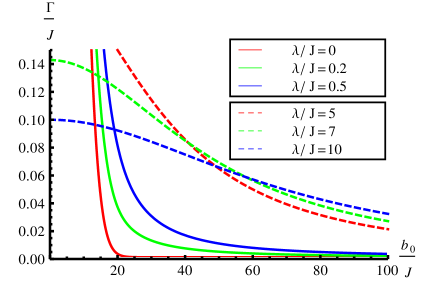
Figure 3: Plotting the diffusion rate $\Gamma_{jk}^{\prime}/J$ as a function of magnetic field gradient $(B_{j}-B_{k})/J$ for a variety of different values of $\lambda/J$. The solid lines show the result in Eq. (49) for case 1. The dashed lines show the result of Eq. (53) for case 2. The actual model is taken to be the same as the Heisenberg model discussed in Section III.

V Discussion and summary

In Section II of this article we have derived a dynamical mean-field theory for systems of spin-half particles on a lattice, in the presence of a nonuniform, external magnetic field. The theory is applicable in the case where the magnetic field gradient between two lattice sites is large compared to the interactions. Additionally, the number of interacting pairs should be large (as is the case for systems of high dimensionality or long range interactions). This condition is necessary to ensure the fluctuations of the effective field at each lattice site are Gaussian (the central limit theorem). One of the most notable approximations we made in deriving this theory of spin diffusion was the exclusion of the summation in Eq. (3). With this sum excluded, we were able to derive a solution to Eq. (3), shown in Eq. (8). We can use this expression for $\sigma_{j}^{+}\sigma_{k}^{-}(t)$, to estimate the size of the summation term in Eq. (3), and thus estimate the error in this approximation.

First, we note from Eqs. (11) and (13), the size of $\sigma_{j}^{+}\sigma_{k}^{-}(t)$ is roughly $\Gamma_{jk}/(2J_{jk}^{\perp})$. Thus, if we substitute our expression for $\sigma_{i}^{+}\sigma_{k}^{-}$ back into Eq. (3), we see that the size of the summation term is approximately $\max\left\{\Gamma_{ni},\Gamma_{nk}\right\}$ where $n$ runs over lattice sites which are mutual neighbors of sites $i$ and $k$. Assuming a certain level of isotropy exists within the system, we conclude that, provided $J_{ik}^{\perp}\gg\Gamma_{ik}$, for all interacting pairs $i$ and $k$, the exclusion of the summation in Eq. (3) is justified. With all conditions satisfied, the equation of motion for the $z$-component of the individual spins is a Langevin equation with additive noise, see Eqs. (12).

If the condition $J_{ik}^{\perp}\gg\Gamma_{ik}$ were not satisfied, and the summation in Eq. (3) could not be justifiably ignored, we would expect a similar analysis to be possible. The summation term would manifest as multiplicative noise in the coefficients $\Gamma_{ik}$ of the Langevin equation (12), as well as the additive noise which we have derived. Further work on this issue however, is still in progress, and the details deferred to a future publication.

The model can be described in terms of simple physical principles, as illustrated in Fig. 1. Interactions between sites $i$ and $j$ can cause spin flip-flopping, i.e. $|i_{\uparrow}j_{\downarrow}\rangle\rightleftarrows|i_{\downarrow}j_{\uparrow}\rangle$. This process occurs when sites $i$ and $j$ have opposite spin, and does not conserve energy when the external field gradient is nonzero (due to the different Zeeman energies). These sites $i$ and $j$ however, also interact with all other neighboring lattice sites (the number of which is assumed to be large). A crucial approximation in our model is to treat all remaining sites as composing an effective bath, or rapidly fluctuating environment in which sites $i$ and $j$ inhabit [see Fig. 1 (b)]. In this way, one can derive the rate at which the spin flip-flopping occurs (we have labelled this quantity $\Gamma_{ij}$), and naturally it will depend on the bath parameters. To be more specific, it depends on the correlation functions between neighboring sites within the bath. The final step then is to determine the rate $\Gamma_{ij}$ that is self-consistent with the bath, i.e. the value of $\Gamma_{ij}$ which yields the same correlation function between neighboring sites, as that from which it was derived.

We find the rate $\Gamma_{ij}$ decays very quickly with increasing field gradient. Equation (16) predicts the rate decays in the same way as a Gaussian distribution. From a numerical study of the cubic Heisenberg lattice (presented in Section III), we expect this prediction to be accurate for $B_{i}-B_{j}\gtrsim 10J_{ij}$ (see Fig. 2). This result implies that the observation of spin diffusion in systems with a very strong magnetic field gradient is likely to be difficult as the diffusion time-scales would be very large.

However, in Section IV we studied the influence of external noise on this rate. The presence of the external noise turns out to be favourable for increasing the diffusion rates. We made use of the same set of assumptions in deriving a second Langevin equation [see Eq. (44)]. In contrast to Section II, the Langevin equation now includes a decay-constant, denoted $\Upsilon_{k}$, which relaxes the system down into a state where the orientation of the magnetic moment is completely random, i.e. $\langle\sigma_{k}^{z}\rangle=0$. Spin flip-flops still occur in the system, and the rate at which they occur; $\Gamma_{ij}^{\prime}$, is affected by the noise. As a general rule, the rate $\Gamma_{ij}^{\prime}$ increases with increasing noise, as is illustrated in Fig. 3. In the limiting case where the external noise is far greater than both the interaction coupling and the external field gradient, we find the rate $\Gamma_{ij}$ decays in the same way as a Cauchy-Lorentz distribution, see Eq. (53). This predicted increase in the rate may help to explain experiments where diffusion has purportedly been observed in systems with very large magnetic field gradients.

VI Acknowledgements

We thank Olexander Chumak, Chris Hammel and Semion Saykin for valuable discussions. The work is supported by the US DOE, and, in part, by ONR and NAS/LPS. Andrew Sykes gratefully acknowledges the support of the U.S. Department of Energy through the LANL/LDRD Program for this work.

Appendix A Perturbation theory for the two-body problem in a fluctuating external field

Consider the following time dependent Hamiltonian describing two spin-half particles located at sites 1 and 2, interacting via an exchange interaction,

$$\hat{H}=B_{1}(t)\sigma_{1}^{z}+B_{2}(t)\sigma_{2}^{z}+J\left(\sigma_{1}^{x}\sigma_{2}^{x}+\sigma_{1}^{y}\sigma_{2}^{y}+\sigma_{1}^{z}\sigma_{2}^{z}\right)$$ (54)

where the external magnetic field $B_{i}(t)=B_{i}+b_{i}(t)$ consists of a constant part and a fluctuating part. We wish to calculate the probability of the spins flip-flopping in time $t$, that is

$$p(t)=\Big{|}\langle 1_{\downarrow}2_{\uparrow}|\hat{U}(t,0)|1_{\uparrow}2_{\downarrow}\rangle\Big{|}^{2}$$ (55)

where $\hat{U}(t,0)$ is the time evolution operator for $\hat{H}$. Splitting the full Hamiltonian up into a noninteracting and an interacting part,

$$\hat{H}_{0} =B_{1}(t)\sigma_{1}^{z}+B_{2}(t)\sigma_{2}^{z}$$ (56)

$$\hat{V} =J\left(\sigma_{1}^{x}\sigma_{2}^{x}+\sigma_{1}^{y}\sigma_{2}^{y}+\sigma_{1}^{z}\sigma_{2}^{z}\right)$$ (57)

and moving to the interaction picture; $|\Psi_{\rm S}(t)\rangle=\hat{U}_{0}(t,0)|\Psi_{\rm I}(t)\rangle$ where $\hat{U}_{0}(t,0)=\exp\left[-i\int_{0}^{t}\hat{H}_{0}(\tau)d\tau\right]$ is the time evolution operator of the noninteracting Hamiltonian. Defining $\hat{V}_{I}(t)=\hat{U}_{0}(t,t_{0})\hat{V}\hat{U}_{0}(t_{0},t)$ and $\hat{U}_{I}(t,0)\exp_{+}\left[-i\int_{0}^{t}\hat{V}_{I}(\tau)d\tau\right]$, where $\exp_{+}$ denotes the usual time-ordered Dyson series sakurai (appropriate for noncommuting $[\hat{V}_{I}(t_{1}),\hat{V}_{I}(t_{2})]\neq 0$ when $t_{1}\neq t_{2}$).

Using this standard formalism, we approximate the full time evolution operator as,

$$\hat{U}(t,0) =\hat{U}_{0}(t,0)\hat{U}_{I}(t,0)$$

$$\simeq\hat{U}_{0}(t,0)\left[1-i\int_{0}^{t}\hat{V}_{I}(\tau)d\tau\right]$$ (58)

by truncating the Dyson series for $\hat{U}_{I}$. Substituting this approximation into Eq. (55) and working through the calculation in a straight-forward manner we arrive at

$$p(t)=4J^{2}\int_{0}^{t}d\tau_{1}\int_{0}^{t}d\tau_{2}\,e^{-2i(B_{1}-B_{2})(\tau_{1}-\tau_{2})+2i\int_{\tau_{1}}^{\tau_{2}}\delta b(s)ds}$$

where $\delta b(s)=b_{1}(s)-b_{2}(s)$. At this point it is convenient to take an average over the fluctuating component of the external field, $e^{2i\int_{\tau_{1}}^{\tau_{2}}\delta b(s)ds}\rightarrow\langle e^{2i\int_{\tau_{1}}^{\tau_{2}}\delta b(s)ds}\rangle$. Assuming these fluctuations are Gaussian, and time-translationally invariant, we find

$$p(t)=\, 4J^{2}\int_{0}^{t}d\tau_{1}\int_{0}^{t}d\tau_{2}\,e^{-2i(B_{1}-B_{2})(\tau_{1}-\tau_{2})}\times$$

$$\quad e^{-4\int_{0}^{|\tau_{1}-\tau_{2}|}ds\langle\delta b(0)\delta b(s)\rangle\left(|\tau_{1}-\tau_{2}|-s\right)}$$

$$=\, 4J^{2}\int_{-t}^{t}d\tau\,\left(t-|\tau|\right)e^{-2i(B_{1}-B_{2})\tau}\times$$

$$\quad e^{-4\int_{0}^{|\tau|}ds\langle\delta b(0)\delta b(s)\rangle\left(|\tau|-s\right)}.$$ (59)

In the limit then, where the time $t$ is much larger than the time scale over which the final term $e^{-4\int_{0}^{|\tau|}ds\langle\delta b(0)\delta b(s)\rangle\left(|\tau|-s\right)}$ decays, the probability becomes

$$p(t)=\, 4tJ^{2}\int_{-\infty}^{\infty}\exp\!\!\Bigg{[}2i(B_{1}-B_{2})s-$$

$$\qquad\left.4\int_{0}^{|s|}\langle\delta b(0)\delta b(s)\rangle\left(|s|-\mu\right)d\mu\right]ds$$ (60)

This probability in Eq. (60) should be compared to the rate at which spin flips are predicted to occur from Eq. (13) in Section II. In making this comparison, we see that the approximations we have applied in deriving the equation of motion (12) for $\sigma_{k}^{z}$ amount to treating all sites other $j$ and $k$ as composing an effective bath (equivalent to a fluctuating external field).

Appendix B Numerical algorithm for solving the integral equation

For our particularly simple choice of $B({\bf r})=\frac{b_{0}}{\sqrt{3}}(r_{x}+r_{y}+r_{z})$, the integral equation we must solve is simply Eq. (24) with $K(\mu)$ given by Eq. (26). From this equation, we wish to determine $\Gamma$ as a function of $b_{0}$, the dependence on $J$ can be removed, by switching to variables $\tilde{\Gamma}=\Gamma/J$ and $\tilde{b}_{0}=b_{0}/J$, such that we have

$$\tilde{\Gamma}=4\int_{-\infty}^{\infty}ds\,e^{\frac{2i\tilde{b}_{0}s}{\sqrt{3}}}e^{-8\int_{0}^{|s|}d\mu\,e^{-6\tilde{\Gamma}\mu}f(2\tilde{\Gamma}\mu)\left(|s|-\mu\right)}.$$

We then search for a root of this equation, by iterating

$$\tilde{\Gamma}^{(n+1)}=4\int_{-\infty}^{\infty}\!\!\!ds\,e^{\frac{2i\tilde{b}_{0}s}{\sqrt{3}}}e^{-8\int_{0}^{|s|}d\mu\,e^{-6\tilde{\Gamma}^{(n)}\mu}f(2\tilde{\Gamma}^{(n)}\mu)\left(|s|-\mu\right)}.$$ (61)

for $n=0,1,2,\ldots$ up to convergence, which in our case was chosen to be $|\tilde{\Gamma}^{(n+1)}-\tilde{\Gamma}^{(n)}|<10^{-4}$. In order to choose a reasonable initial prediction for $\tilde{\Gamma}^{(0)}$ we begin the algorithm at $\tilde{b}_{0}=20$, and define

$$\tilde{\Gamma}^{(0)}\simeq 4\sqrt{\frac{\pi}{20}}e^{-\tilde{b}_{0}^{2}/(60)}.$$ (62)

Once the algorithm has converged, we decrease $b_{0}$ by a small amount and use our previous prediction for $\tilde{\Gamma}$ as our new $\tilde{\Gamma}^{(0)}$.

Appendix C The issue regarding convergence/divergence of $\Gamma$ as $b_{0}\rightarrow 0$

As the field gradient decreases in a particular direction, the rate at which spin flip-flops occur in that particular direction increases, see Figure 2. It is not clear, a priori, that the rate will remain finite in the limit of vanishing gradient. Consider, for example, the RHS of Eq. (24) (and set $J=1$). We can rewrite this in terms of the Fourier transform of $K(\mu)=\frac{1}{2\pi}\int e^{-i\omega\mu}\tilde{K}(\omega)d\omega$, and we are only interested in the case where $b_{0}=0$, so we find,

$${\rm RHS}(\Gamma)=4\int_{\mathbb{R}}\exp\left[-\frac{2}{\pi}\int_{\mathbb{R}}\tilde{K}(\omega)\frac{1-\cos(\omega|s|)}{\omega^{2}}d\omega\right]ds.$$ (63)

Next we define $\gamma=\mu\Gamma$, in which case

$$\tilde{K}(\omega) =2\int_{\mathbb{R}}\frac{d\gamma}{\Gamma}e^{i\frac{\omega\gamma}{\Gamma}}e^{-6\gamma}f(2\gamma)$$

$$=\frac{2}{\Gamma}H\left(\frac{\omega}{\Gamma}\right)$$ (64)

where $H(x)=\int_{\mathbb{R}}d\gamma\,e^{ix\gamma}e^{-6\gamma}f(2\gamma)$. The RHS therefore becomes,

$${\rm RHS}(\Gamma)=4\int_{\mathbb{R}}\exp\left[-\frac{4}{\pi}\int_{\mathbb{R}}d\eta\,H(\eta)\frac{1-\cos(\Gamma\eta|s|)}{\Gamma^{2}\eta^{2}}\right]ds.$$ (65)

where we defined $\eta=\omega/\Gamma$. Now we make the assumption that $\Gamma$ does become very large, in this limit we find

$$\frac{1-\cos(\Gamma\eta|s|)}{\Gamma^{2}\eta^{2}}\rightarrow\frac{\pi|s|}{\Gamma}\delta(\eta)$$ (66)

and therefore

$${\rm RHS}(\Gamma)\rightarrow\frac{2\Gamma}{H(0)}$$ (67)

for large $\Gamma$. The quantity $H(0)$ can be calculated numerically to be $H(0)\eqsim 2.33$, thereby indicating that the slope of the RHS is $<1$ for large $\Gamma$. From this we conclude that a finite value of $\Gamma$ will exist at $b_{0}=0$ which satisfies Eq. (24).

References

• (1) A. Abragam, Principles of Nuclear Magnetism (Oxford University Press, 1961).
• (2) C. P. Slichter, Principles of Magnetic Resonance (Springer-Verlag, 1978).
• (3) J. R. Klauder and P. W. Anderson, Phys. Rev. 125, 912 (1962).
• (4) R. de Sousa and S. Das Sarma, Phys. Rev. B 68, 115322 (2003).
• (5) W. M. Witzel and S. Das Sarma, Phys. Rev. B 74, 033322 (2006).
• (6) S. K. Saikin W. Yao and L. J. Sham, Phys. Rev. B 75, 125314 (2007).
• (7) A. A. Tarasenko, P. M. Tomchuk and A. A. Chumak, Fluctuatsii v ob’eme i na poverhnosti tverdyh tel (in Russian, Kiev, Naukova Dumka, 1992).
• (8) Sh. Kogan, Electronic noise and fluctuations in solids, (Cambridge University Press, 1996).
• (9) K. Blum, Density matrix theory and its applications (Springer Series on Atomic, Optical and Plasma Physics, 1996).
• (10) Gradshtein and Ryzhik, Table of integrals, series and products (Academic press, 2000).
• (11) J. J. Sakurai, Modern quantum mechanics (Addison-Wesley Publishing, 1994).
• (12) M. Abramowitz and I. A. Stegun, Handbook of mathematical functions, (US Govt Printing Office, 1972).