Thermodynamic Tree: The Space of Admissible Paths

Abstract

Is a spontaneous transition from a state $x$ to a state $y$ allowed by thermodynamics? Such a question arises often in chemical thermodynamics and kinetics. We ask the more formal question: is there a continuous path between these states, along which the conservation laws hold, the concentrations remain non-negative and the relevant thermodynamic potential $G$ (Gibbs energy, for example) monotonically decreases? The obvious necessary condition, $G(x)\geq G(y)$, is not sufficient, and we construct the necessary and sufficient conditions. For example, it is impossible to overstep the equilibrium in 1-dimensional (1D) systems (with $n$ components and $n-1$ conservation laws). The system cannot come from a state $x$ to a state $y$ if they are on the opposite sides of the equilibrium even if $G(x)>G(y)$. We find the general multidimensional analogue of this 1D rule and constructively solve the problem of the thermodynamically admissible transitions.

We study dynamical systems, which are given in a positively invariant convex polyhedron $D$ and have a convex Lyapunov function $G$. An admissible path is a continuous curve in $D$ along which $G$ does not increase. For $x,y\in D$, $x\succsim y$ ($x$ precedes $y$) if there exists an admissible path from $x$ to $y$ and $x\sim y$ if $x\succsim y$ and $y\succsim x$. The tree of $G$ in $D$ is a quotient space $D/\sim$. We provide an algorithm for the construction of this tree. In this algorithm, the restriction of $G$ onto the 1-skeleton of $D$ (the union of edges) is used. The problem of existence of admissible paths between states is solved constructively. The regions attainable by the admissible paths are described.

1 Introduction

1.1 Motivation, ideas and a simple example

“Applied dynamical systems” are models of real systems. The available information about the real systems is incomplete and uncertainties of various types are encountered in the modeling. Often, we view them as errors: errors in the model structure, errors in coefficients, in the state observation and many others. Nevertheless, there is an order in this world of errors: some information is more reliable, we trust in some structures more and even respect them as laws. Some other data are less reliable. There is an hierarchy of reliability, our knowledge and beliefs (described, for example by R. Peierls [53] for model making in physics). Extracting as many consequences from the more reliable data either without or before use of the less reliable information is a task which arises naturally.

In our paper, we study dynamical systems with a strictly convex Lyapunov function $G$ defined in a positively invariant convex polyhedron $D$. For them, we analyze the admissible paths, along which $G$ decreases monotonically, and find the states that are attainable from the given initial state along the admissible paths. The main area of applications of these systems is chemical kinetics and thermodynamics. The motivation of our research comes from the hierarchy of reliability of the information in these applications.

Let us discuss the motivation in more detail. In chemical kinetics, we can rank the information in the following way. First of all, the list of reagents and conservation laws should be known. Let the reagents be $A_{1},A_{2},\ldots,A_{n}$. The non-negative real variable $N_{i}\geq 0$, the amount of $A_{i}$ in the mixture, is defined for each reagent, and $N$ is the vector of composition with coordinates $N_{i}$. The conservation laws are presented by the linear balance equations:

$$b_{i}(N)=\sum_{j=1}^{n}a_{i}^{j}N_{j}={\rm const}\;\;(i=1,\ldots,m)\,.$$ (1)

We assume that the linear functions $b_{i}(N)$ ($i=1,\ldots,m$) are linearly independent.

The list of the components together with the balance conditions (1) is the first part of the information about the kinetic model. This determines the space of states, the polyhedron $D$ defined by the balance equations (1) and the positivity inequalities $N_{i}\geq 0$. This is the background of kinetic models and any further development is less reliable. The polyhedron $D$ is assumed to be bounded. This means that there exist such coefficients $\lambda_{i}$ that the linear combination $\sum_{i}\lambda_{i}b_{i}(N)$ has strictly positive coefficients: $\sum_{i}\lambda_{i}a_{i}^{j}>0$ for all $j=1,\ldots,n$.

The thermodynamic functions provide us with the second level of information about the kinetics. Thermodynamic potentials, such as the entropy, energy and free energy are known much better than the reaction rates and, at the same time, they give us some information about the dynamics. For example, the entropy increases in isolated systems. The Gibbs free energy decreases in closed isothermal systems under constant pressure, and the Helmholtz free energy decreases under constant volume and temperature. Of course, knowledge of the Lyapunov functions gives us some inequalities for vector fields of the systems’ velocity but the values of these vector fields remain unknown. If there are some external fluxes of energy or non-equilibrium substances then the thermodynamic potentials are not Lyapunov functions and the systems do not relax to the thermodynamic equilibrium. Nevertheless, the inequality of positivity of the entropy production persists and this gives us useful information even about the open systems. Some examples are given in [26, 28].

The next, third part of the information about kinetics is the reaction mechanism. It is presented in the form of the stoichiometric equations of the elementary reactions:

$$\sum_{i}\alpha_{\rho i}A_{i}\to\sum_{i}\beta_{\rho i}A_{i}\,,$$ (2)

where $\rho=1,\ldots,m$ is the reaction number and the stoichiometric coefficients $\alpha_{\rho i},\beta_{\rho i}$ ($i=1,\ldots,n$) are nonnegative integers.

A stoichiometric vector $\gamma_{\rho}$ of the reaction (2) is a $n$-dimensional vector with coordinates $\gamma_{\rho i}=\beta_{\rho i}-\alpha_{\rho i}$, that is, ‘gain minus loss’ in the $\rho$th elementary reaction.

The concentration of $A_{i}$ is an intensive variable $c_{i}=N_{i}/V$, where $V>0$ is the volume. The vector $c=N/V$ with coordinates $c_{i}$ is the vector of concentrations. A non-negative intensive quantity, $r_{\rho}$, the reaction rate, corresponds to each reaction (2). The kinetic equations in the absence of external fluxes are

$$\frac{{\mathrm{d}}N}{{\mathrm{d}}t}=V\sum_{\rho}r_{\rho}\gamma_{\rho}\,.$$ (3)

If the volume is not constant then equations for concentrations include $\dot{V}$ and have different form.

For perfect systems and not so fast reactions the reaction rates are functions of concentrations and temperature given by the mass action law and by the generalized Arrhenius equation. A special relation between the kinetic constants is given by the principle of detailed balance: For each value of temperature $T$ there exists a positive equilibrium point where each reaction (2) is equilibrated with its reverse reaction. This principle was introduced for collisions by Boltzmann in 1872 [10]. Wegscheider introduced this principle for chemical kinetics in 1901 [67]. Einstein in 1916 used it in the background for his quantum theory of emission and absorption of radiation [17]. Later, it was used by Onsager in his famous work [51]. For a recent review see [30].

At the third level of reliability of information, we select the list of components and the balance conditions, find the thermodynamic potential, guess the reaction mechanism, accept the principle of detailed balance and believe that we know the kinetic law of elementary reactions. However, we still do not know the reaction rate constants.

Finally, at the fourth level of available information, we find the reaction rate constants and can analyze and solve the kinetic equations (3) or their extended version with the inclusion of external fluxes.

Of course, this ranking of the available information is conventional, to a certain degree. For example, some reaction rate constants may be known even better than the list of intermediate reagents. Nevertheless, this hierarchy of the information availability, list of components – thermodynamic functions – reaction mechanism – reaction rate constants, reflects the real process of modelling and the stairs of available information about a reaction kinetic system.

It seems very attractive to study the consequences of the information of each level separately. These consequences can be also organized ‘stairwise’. We have the hierarchy of questions: how to find the consequences for the dynamics (i) from the list of components, (ii) from this list of components plus the thermodynamic functions of the mixture, and (iii) from the additional information about the reaction mechanism.

The answer to the first question is the description of the balance polyhedron $D$. The balance equations (1) together with the positivity conditions $N_{i}\geq 0$ should be supplemented by the description of all the faces. For each face, some $N_{i}=0$ and we have to specify which $N_{i}$ have zero value. The list of the corresponding indices $i$, for which $N_{i}=0$ on the face, $I=\{i_{1},\ldots,i_{k}\}$, fully characterizes the face. This problem of double description of the convex polyhedra [49, 14, 21] is well known in linear programming.

The list of vertices [6] and edges with the corresponding indices is necessary for the thermodynamic analysis. This is the 1-skeleton of $D$. Algorithms for the construction of the 1-skeletons of balance polyhedra as functions of the balance values were described in detail in 1980 [26]. The related problem of double description for convex cones is very important for the pathway analysis in systems biology [58, 22].

In this work, we use the 1-skeleton of $D$, but the main focus is on the second step, i.e. on the consequences of the given thermodynamic potentials. For closed systems under classical conditions, these potentials are the Lyapunov functions for the kinetic equations. For example, for perfect systems we assume the mass action law. If the equilibrium concentrations $c^{*}$ are given, the system is closed and both temperature and volume are constant then the function

$$G=\sum_{i}c_{i}(\ln({c_{i}}/{c_{i}^{*}})-1)$$ (4)

is the Lyapunov function; it should not increase in time. The function $G$ is proportional to the free energy $F=RTG+{\rm const}$ (for detailed information about the Lyapunov functions for kinetic equations under classical conditions see the textbook [68] or the recent paper [33]).

If we know the Lyapunov function $G$ then we have the necessary conditions for the possibility of transition from the vector of concentrations $c$ to $c^{\prime}$ during the non-stationary reaction: $G(c)\geq G(c^{\prime})$ because the inequality $G(c(t_{0}))\geq G(c(t_{0}+t))$ holds for any time $t\geq 0$.

The inequality $G(c)\geq G(c^{\prime})$ is necessary if we are to reach $c^{\prime}$ from the initial state $c$ by a thermodynamically admissible path, but it is not sufficient because in addition to this inequality there are some other necessary conditions. The simplest and most famous of them is: if $D$ is one-dimensional (a segment) then the equilibrium $c^{*}$ divides this segment into two parts and both $c(t_{0})$ and $c(t_{0}+t)$ ($t>0$) are always on the same side of the equilibrium.

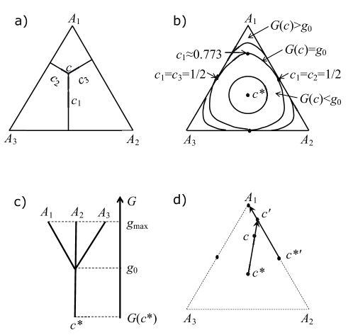
Fig. 1: The balance simplex (a), the levels of the Lyapunov function (b) and the thermodynamic tree (c) for the simple system of three components, $A_{1},A_{2},A_{3}$. Algorithm for finding a vertex $v\succsim c$ (d).

In 1D systems the overstepping of the equilibrium is forbidden. It is impossible to overstep a point in dimension one, but it is possible to circumvent a point in higher dimensions. Nevertheless, in any dimension the inequality $G(c)\geq G(c^{\prime})$ is not sufficient if we are to reach $c^{\prime}$ from the initial state $c$ along an admissible path. Some additional restrictions remain in the general case as well. A two-dimensional example is presented in Fig. 1. Let us consider the mixture of three components, $A_{1,2,3}$ with the only conservation law $c_{1}+c_{2}+c_{3}=b$ (we take for illustration $b=1$) and the equidistribution in equilibrium $c_{1}^{*}=c_{2}^{*}=c_{3}^{*}=1/3$. The balance polyhedron is the triangle (Fig. 1a). In Fig. 1b the level sets of

$$G=\sum_{i=1}^{3}c_{i}(\ln(3c_{i})-1)$$

are presented. This function achieves its minimum at equilibrium, $G(c^{*})=-1$. On the edges, the function $G$ achieves its conditional minimum, $g_{0}$, in the middles, and $g_{0}=\ln(3/2)-1$. $G$ reaches its maximal value, $g_{\max}=\ln 3-1$, at the vertices.

If $G(c^{*})<g\leq g_{0}$ then the level set $G(c)=g$ is connected. If $g_{0}<g\leq g_{\max}$ then the corresponding level set $G(c)=g$ consists of three components (Fig. 1b). The critical value is $g=g_{0}$. The critical level $G(c)=g_{0}$ consists of three arcs. Each arc connects two middles of the edges and divides $D$ in two sets. One of them is convex and includes two vertices, the other includes the remaining vertex.

A thermodynamically admissible path is a continuous curve along which $G$ does not increase. Therefore, such a path cannot intersect these arcs ‘from inside’, i.e. from values $G(c)\leq g_{0}$ to bigger values, $G(c)>g_{0}$. For example, if an admissible path starts from the state with 100% of $A_{2}$, then it cannot intersect the arc that separates the vertex with 100% $A_{1}$ from two other vertices. Therefore, any vertex cannot be reached from another one and if we start from 100% of $A_{2}$ then the reaction cannot overcome the threshold $\sim$77.3% of $A_{1}$, that is the maximum of $c_{1}$ on the corresponding arc (Fig. 1b). This is an example of the 2D analogue of the 1D prohibition of overstepping of equilibrium.

For $x,y\in D$, $x\succsim y$ ($x$ precedes $y$) if there exists a thermodynamically admissible path from $x$ to $y$, and $x\sim y$ if $x\succsim y$ and $y\succsim x$. The equivalence classes with respect to $x\sim y$ in $D$ are the connected components of the level sets $G(c)=g$. The quotient space $\mathcal{T}=D/\sim$ is the space of these connected components. For the canonical projection we use the standard notation $\pi:D\to\mathcal{T}$. This is the tree of the connected components of the level sets of $G$. (Here “tree” stands for a one dimensional continuum, a sort of dendrites [13], and not for a tree in the sense of the graph theory.)

If $x\sim y$ then $G(x)=G(y)$. Therefore, we can define the function $G$ on the tree: $G(\pi(c))=G(c)$. It is convenient to draw this tree on the plane with the vertical coordinate $g=G(x)$ (Fig. 1c). The equilibrium $c^{*}$ corresponds to a root of this tree, $\pi(c^{*})$. If $G(c^{*})<g\leq g_{0}$ then the level set $G(c)=g$ corresponds to one point on the tree. The level $G(c)=g_{0}$ corresponds to the branching point, and each connected component of the level sets $G(c)=g$ with $g_{0}<g\leq g_{\max}$ corresponds to a separate point on the tree. The terminal points (“leaves” with $g>g_{0}$) of the tree correspond to the vertices of $D$.

An ordered segment $[x,y]$ or $[y,x]$ ($x\succsim y$) on the tree $\mathcal{T}$ consists of such points $z$ that $x\succsim z\succsim y$. A continuous curve $\varphi:[0,1]\to D$ is an admissible path if and only if its image $\pi\circ\varphi:[0,1]\to\mathcal{T}$ is a path that goes monotonically down in the coordinate $g$. Such a monotonic path in $\mathcal{T}$ from a point $x$ to the root is just a segment $[x,\pi(c^{*})]$. On this segment, each point $y$ is unambiguously characterized by $g=G(y)$. Therefore, if for $c\in D$ we know the value $G(c)$ and a vertex $v\succsim c$, then we can unambiguously describe the image of $c$ on the tree: $\pi(c)$ is the point on the segment $[\pi(v),\pi(c^{*})]$ with the given value of $G$, $g=G(c)$.

We can find a vertex $v\succsim c$ by a chain of central projections: the first step is the central projection of $c$ onto the border of $D$ with center $c^{*}$. The result is the point $c^{\prime}$ on a face (in Fig. 1d this is the point $c^{\prime}$ on an edge). The second step is the central projection of the point $c^{\prime}$ onto the border of the face with the center at the partial equilibrium ${c^{*}}^{\prime}$ (that is, the minimizer of $G$ on the face) and so on (Fig. 1d). If the projection on a face is the partial equilibrium then for any vertices $v$ of the face $v\succsim c$. In particular, if the face is a vertex $v$ then $v\succsim c$. For a simple example presented in Fig. 1d this is the vertex $A_{1}$.

In this paper, we extend these ideas and observations to any dynamical system, which is given in a positively invariant convex polyhedron and has there a strictly convex Lyapunov function. The class of chemical kinetic equations for closed systems provides us standard and practically important examples of the systems of this class.

1.2 A bit of history

It seems attractive to use an attainable region instead of the single trajectory in situations with incomplete information or with information with different levels of reliability. Such situations are typical in many areas of science and engineering. For example, the theory for the continuous–time Markov chain is presented in [2, 27] and for the discrete–time Markov chains in [3].

Perhaps, the first celebrated example of this approach was developed in biological kinetics. In 1936, A.N. Kolmogorov [40] studied the dynamics of interacting populations of prey ($x$) and predator ($y$) in the general form:

$$\dot{x}=xS(x,y),\;\;\dot{y}=yW(x,y)$$

under monotonicity conditions: $\partial S(x,y)/\partial y<0$, $\partial W(x,y)/\partial y<0$. The zero isoclines, given by equations $S(x,y)=0$ or $W(x,y)=0$, are graphs of two functions $y(x)$. These isoclines divide the phase space into compartments with curvilinear borders. The geometry of the intersection of the zero isoclines, together with some monotonicity conditions, contain important information about the system dynamics that we can find [40] without exact knowledge of the kinetic equations. This approach to population dynamics was applied to various problems [45, 7]. The impact of this work on population dynamics was analyzed in the review [62].

In 1964, Horn proposed to analyze the attainable regions for chemical reactors [36]. This approach became popular in chemical engineering. It was applied to the optimization of steady flow reactors [23], to batch reactor optimization without knowledge of detailed kinetics [19], and for optimization of the reactor structure [34]. An analysis of attainable regions is recognized as a special geometric approach to reactor optimization [18] and as a crucially important part of the new paradigm of chemical engineering [35].

Many particular applications were developed, from polymerization [63] to particle breakage in a ball mill [47] and hydraulic systems [28]. Mathematical methods for the study of attainable regions vary from Pontryagin’s maximum principle [46] to linear programming [38], the Shrink-Wrap algorithm [43], and convex analysis. In 1979 it was demonstrated how to utilize the knowledge about partial equilibria of elementary processes to construct the attainable regions [24]. The attainable regions significantly depend on the reaction mechanism and it is possible to use them for the discrimination of mechanisms [29].

Thermodynamic data are more robust than the reaction mechanism. Hence, there are two types of attainable regions. The first is the thermodynamic one, which use the linear restrictions and the thermodynamic functions [25]. The second is generated by thermodynamics and stoichiometric equations of elementary steps (but without reaction rates) [24, 31]. R. Shinnar and other authors [61] rediscovered this approach. There was even an open discussion about priority [9].

Some particular classes of kinetic systems have rich families of the Lyapunov functions. Krambeck [41] studied attainable regions for linear systems and the $l_{1}$ Lyapunov norm instead of the entropy. Already simple examples demonstrate that the sets of distributions which are accessible from a given initial distribution by linear kinetic systems (Markov processes) with a given equilibrium are, in general, non-convex polytopes [24, 27, 70]. The geometric approach to attainability was developed for all the thermodynamic potentials and for open systems as well [26]. Partial results for chemical kinetics and some other engineering systems are summarized in [68, 28].

The tree of the level set components for differentiable functions was introduces in the middle of the 20 century by Adelson-Velskii and Kronrod [1, 42] and Reeb [56]. Sometimes these trees are called the Reeb trees [20] but from the historical point of view it may be better to call them the Adelson-Velskii – Kronrod – Reeb (or AKR) trees. These trees were essentially used by Kolmogorov and Arnold [4] in solution of the Hilbert’s superposition problem (the ideas, their relations to dynamical systems and role in the Arnold’s scientific life are discussed in his lecture [5]).

The general Reeb graph can be defined for any topological space $X$ and real function $f$ on it. It is the quotient space of $X$ by the equivalence relation “$\sim$” defined by $x\sim y$ holds if and only if $f(x)=f(y)$ and $x$, $y$ are in the same connected component of $f^{-1}(f(x))$. Of course, this “graph” is again not a discrete object from the graph theory but a topological space. It has application in differential topology (Morse theory [48]), in topological shape analysis and visualization [20, 39], in data analysis [64] and in asymptotic analysis of fluid dynamics [44, 59]. The books [20, 39] include many illustration of the Reeb graphs. The efficient mesh-based methods for the computation of the graphs of level set components are developed for general scalar fields on 2- and 3-dimensional manifolds [16].

Some time ago the tree of entropy in the balance polyhedra was rediscovered as an adequate tool for representation of the attainable regions in chemical thermodynamics [25, 26]. It was applied to analysis of various real systems [37, 69]. Nevertheless, some of the mathematical backgrounds of this approach were delayed in development and publications. Now, the thermodynamically attainable regions are in extensive use in chemical engineering and beyond [18, 19, 23, 28, 34, 35, 36, 37, 38, 41, 43, 46, 47, 60, 61, 63, 69]. In this paper we aim to provide the complete mathematical background for the analysis of the thermodynamically attainable regions. For this purpose, we construct the trees of strictly convex functions in a convex polyhedron. This problem allows a general meshless solution in higher dimensions because topological and geometrical simplicity (the domain $D$ is a convex polyhedron and the function $G$ is strictly convex in D). In this paper, we present this solution in detail.

1.3 The problem of attainability and its solution

Let us formulate precisely the problem of attainability and its solution before the exposition of all technical details and proofs. Our results are applicable to any dynamical system that obeys a continuous strictly convex Lyapunov function in a positively invariant convex polyhedron. The situations with uncertainty, when the specific dynamical system is not given with an appropriate accuracy but the Lyapunov function is known, give a natural area of application of these results.

Here and below, $D$ is a convex polyhedron in $\mathbb{R}^{n}$, $D_{0}$ consists of the vertices of $D$, $D_{1}$ is the union of the closed edges of $D$, that is, the 1-skeleton of $D$, and $\widetilde{D_{1}}$ is the graph whose vertices correspond to the vertices of $D$ and edges correspond to the edges of $D$, (the graph of the 1-skeleton) of $D$. We use the same notations for vertices and edges of $D$ and $\widetilde{D_{1}}$.

Let a real continuous function $G$ be given in $D$. We assume that $G$ is strictly convex in $D$ [57]. Let $x^{*}$ be the minimizer of $G$ in $D$ and let $g^{*}=G(x^{*})$ be the corresponding minimal value.

The level set $S_{g}=\{x\in D\,|\,G(x)=g\}$ is closed and the sublevel set $U_{g}=\{x\in D\,|\,G(x)<g\}$ is open in $D$ (i.e. it is the intersection of an open subset of $\mathbb{R}^{n}$ with $D$).

Let us transform $\widetilde{D_{1}}$ into a labeled graph. Each vertex $v\in D_{0}$ is labeled by the value $\gamma_{v}=G(v)$ and each edge $e=[v,w]\subset D_{1}$ is labeled by the minimal value of $G$ on the segment $[v,w]\subset D$, $g_{e}=\min_{[v,w]}G(x)$. The vertices and edges of $\widetilde{D_{1}}$ are labeled by the same numbers as the correspondent vertices and edges of $D_{1}$. By definition, the graph $\widetilde{D_{1}}\setminus U_{g}$ consists of the vertices and edges of $\widetilde{D_{1}}$, whose labels $\gamma\geq g$.

The graph $\widetilde{D_{1}}\setminus U_{g}$ depends on $g$ but this is a piecewise constant dependence. It changes only at $g=\gamma$, where $\gamma$ are some of the labels of the graph $\widetilde{D_{1}}$. Therefore, it is not necessary to find this graph and to analyze connectivity in it for each value $G(y)=g$.

Definition 1.

A continuous path $\varphi[0,1]\to D$ is admissible if the function $G(\varphi(x))$ does not increase on $[0,1]$. For $x,y\in D$, $x\succsim y$ ($x$ precedes $y$) if there exists an admissible path $\varphi[0,1]\to D$ with $\varphi(0)=x$ and $\varphi(1)=y$; $x\sim y$ if $x\succsim y$ and $y\succsim x$.

The relation “$\succsim$” is transitive. It is a preorder on $D$. The relation “$\sim$” is an equivalence.

Definition 2.

The tree of $G$ in $D$ is the quotient space $\mathcal{T}=D/\sim$.

The equivalence classes of $\sim$ are the path-connected components of the level sets $S_{g}$. For the natural projection of $D$ on $\mathcal{T}$ we use the notation $\pi:D\to\mathcal{T}$. We denote by $\pi^{-1}(z)\subset D$ the set of preimages of $z\in\mathcal{T}$. The preorder “$\succsim$” on $D$ transforms into a partial order on $\mathcal{T}$: $\pi(x)\succsim\pi(y)$ if and only if $x\succsim y$. We call $\mathcal{T}$ also the thermodynamic tree keeping in mind the thermodynamic applications. The “tree” $\mathcal{T}$ is a 1D continuum. We have to distinguish this continuum from trees in the graph-theoretic sense which have the same graphical representation but are discrete objects. In Sec. 3.2 (“Coordinates on the thermodynamic tree”) we describe the tree structure of this continuum. It includes the root, the edges, the branching points and leaves but the edges are represented as the real line segments.

Definition 3.

Let $x,y\in\mathcal{T}$, $x\succsim y$. An ordered segment $[x,y]$ (or $[y,x]$) consists of such points $z\in\mathcal{T}$ that $x\succsim z\succsim y$.

In Sec. 3 we prove that any ordered segment $[x,y]$ ($x\neq y$) in $\mathcal{T}$ is homeomorphic to $[0,1]$. A continuous curve $\varphi:[0,1]\to D$ is an admissible path if and only if its image $\pi\circ\varphi:[0,1]\to\mathcal{T}$ is monotonic in the partial order on $\mathcal{T}$. Such a monotonic path in $\mathcal{T}$ from $x$ to $y$ ($x\succsim y$) is just a path along a segment $[x,y]$. Each point $z$ on this segment is unambiguously characterized by the value of $G(z)$.

We also use the notation $[x,y]$ for the usual closed segments in $\mathbb{R}^{n}$ with ends $x,y$: $[x,y]=\{\lambda x+(1-\lambda)y\,|\,\lambda\in[0,1]\}$. The degenerated segment $[x,x]$ is just a point $\{x\}$. The segments without one end are $(x,y]$ and $[x,y)$ and $(x,y)$ is the segment in $\mathbb{R}^{n}$ without both ends.

The attainability problem: Let $x,y\in D$ and $G(x)\geq G(y)$. Is $y$ attainable from $x$ by an admissible path?

The solution of the attainability problem can be found in several steps:

1. Find two vertices of $D$, $v_{x}$ and $v_{y}$, that precede $x$ and $y$, correspondingly. Such vertices always exist. There may be several such vertices in $D$. We can use any of them.

2. Construct the graph $\widetilde{D_{1}}\setminus U_{G(y)}$ by deletion from $\widetilde{D_{1}}$ all the elements with the labels $\gamma<G(y)$.

3. $y$ is attainable from $x$ by an admissible path if and only if $v_{x}$ and $v_{y}$ are connected in the graph $\widetilde{D_{1}}\setminus U_{G(y)}$.

So, to check the existence of an admissible path from $x$ to $y$ we should check the inequality $G(x)\geq G(y)$ (the necessary condition) then go up in $G$ values and find the vertices, $v_{x}$ and $v_{y}$, that precede $x$ and $y$, correspondingly (such vertices always exist). Then we should go down in $G$ values to $G(y)$ and check whether the vertices $v_{x}$ and $v_{y}$ are connected in the graph $\widetilde{D_{1}}\setminus U_{G(y)}$. The classical problem of determining whether two vertices in a graph are connected may be solved by many search algorithms [52, 50], for example, by the elementary breadth–first or depth–first search algorithms.

The procedure “find a vertex $v_{x}\in D_{0}$ that precedes $x\in D$” can be implemented as follows:

1. If $x=x^{*}$ then any vertex $v\in D_{0}$ precedes $x$.

2. If $x\neq x^{*}$ then consider the ray $r_{x}=\{x^{*}+\lambda(x-x^{*})\,|\,\lambda\geq 0\}$. The intersection $r_{x}\cap D$ is a closed segment $[x^{*},x^{\prime}]$. We call $x^{\prime}$ the central projection of $x$ onto the border of $D$ with the center $x^{*}$; $x^{\prime}\succsim x$.

3. The central projection $x^{\prime}$ always belongs to an interior of a face $D^{\prime}$ of $D$, $0\leq\dim D^{\prime}<\dim D$. If $\dim D^{\prime}>0$ then set $x:=x^{\prime}$, $D:=D^{\prime}$, $x^{*}:={\rm argmin}\{G(z)\,|\,z\in D^{\prime}\}$ and go to step 1.

4. If $\dim D^{\prime}=0$ then it is a vertex $v\succsim x$ we are looking for.

The dimension of the face decreases at each step, hence, after not more than $\dim D-1$ steps we will definitely obtain the desired vertex. A simple example is presented in Fig. 1d.

The information about all connected components of $\widetilde{D_{1}}\setminus U_{g}$ for all values of $g$ is summarized in the tree of $G$ in $D$, $\mathcal{T}$ (Definition 2). The tree $\mathcal{T}$ can be described as follows (Theorem 15): it is the space of pairs $(g,M)$, where $g\in[\min_{D}G(x),\max_{D}G(x)]$ and $M$ is a connected component of $\widetilde{D_{1}}\setminus U_{g}$, with the partial order relation: $(g,M)\succsim(g^{\prime},M^{\prime})$ if $g\geq g^{\prime}$ and $M\subseteq M^{\prime}$. For $x,y\in D$, $x\succsim y$ if and only if $\pi(x)\succsim\pi(y)$.

The tree $\mathcal{T}$ may be constructed gradually, by descending from the maximal value of $G$, $g=g_{\max}$ (Sec. 3.3). At $g=g_{\max}$, the graph $\widetilde{D_{1}}\setminus U_{g}$ consists of the isolated vertices with the labels $\gamma=g_{\max}$ (generically, this is one vertex). Going down in $g$, we add to $\widetilde{D_{1}}\setminus U_{g}$ the elements, vertices and edges, in descending order of their labels. After adding each element we record the changes in the connected components of $\widetilde{D_{1}}\setminus U_{g}$.

For each point $z\in\mathcal{T}$, $z=(g,M)$, its preimage in $D$, $\pi^{-1}(g,M)$, may be described by the equation $G(x)=g$ supplemented by a set of linear inequalities. Computationally, these linear inequalities can be produced by a convex hull operation from a finite set. This finite set is described explicitly in Sec. 3.4.

For each point $z=(g,M)$ the set of all $z^{\prime}=(g^{\prime},M^{\prime})$ attainable by admissible paths from $z$ has a simple description, $g^{\prime}\leq g$, $M^{\prime}\supseteq M$.

The tree of $G$ in $D$ provides a workbench for the analysis of various questions about admissible paths. It allows us to reduce the $n$-dimensional problems in $D$ to some auxiliary questions about such 1D or even discrete objects as the tree $\mathcal{T}$ and the labeled graph $\widetilde{D_{1}}$. For example, we use the thermodynamic tree to solve the following problem of attainable sets: For a given $x\in D$ describe the set of all $y\precsim x$ by a system of inequalities. For this purpose, we find the image of $x$ in $\mathcal{T}$, $\pi(x)$, then define the set of all points attainable by admissible paths from $\pi(x)$ in $\mathcal{T}$ and, finally, describe the preimage of this set in $D$ by the system of inequalities (Sec. 3.4).

1.4 The structure of the paper

In Sec. 2, we present several auxiliary propositions from convex geometry. We constructively describe the result of the cutting of a convex polyhedron $D$ by a convex set $U$: The description of the connected components of $D\setminus U$ is reduced to the analysis of the 1D continuum $D_{1}\setminus U$, where $D_{1}$ is the 1-skeleton of $D$.

In Sec. 3, we construct the tree of level set components of a strictly convex function $G$ in the convex polyhedron $D$ and study the properties of this tree. The main result of this section is the algorithm for construction of this tree (Sec. 3.3). This construction is applied to the description of the attainable sets in Sec. 3.4. These sections include some practical recipes and it is possible to read them independently, immediately after Introduction. Several examples of the thermodynamic trees for chemical systems are presented in Sec. 4.

2 Cutting of a polyhedron $D$ by a convex set $U$

2.1 Connected components of $D\setminus U$ and of $D_{1}\setminus U$

Let $D$ be a convex polyhedron in $\mathbb{R}^{n}$. We use the notations: ${\rm Aff}(D)$ is the minimal linear manifold that includes $D$; $d=\dim{\rm Aff}(D)=\dim D$ is the dimension of $D$; $ri(D)$ is the interior of $D$ in ${\rm Aff}(D)$; $r\partial(D)$ is the border of $D$ in ${\rm Aff}(D)$.

For $P,Q\subset\mathbb{R}^{n}$ the Minkowski sum is $P+Q=\{x+y\,|\,x\in P,y\in Q\}$. The convex hull (conv) and the conic hull (cone) of a set $V\subset\mathbb{R}^{n}$ are:

$${\rm conv}(V)=\left\{\sum_{i=1}^{q}\lambda_{i}v_{i}\,\left|\,q>0,\,v_{1},\ldots,v_{q}\in V,\,\lambda_{1},\ldots\lambda_{q}>0,\,\sum_{i=1}^{q}\lambda_{i}=1\right.\right\}\,;$$

$${\rm cone}(V)=\left\{\left.\sum_{i=1}^{q}\lambda_{i}v_{i}\,\right|\,q\geq 0,\,v_{1},\ldots,v_{q}\in V,\,\lambda_{1},\ldots\lambda_{q}>0,\,\right\}\,.$$

For a set $D\subset\mathbb{R}^{n}$ the following two statements are equivalent (the Minkowski–Weyl theorem):

1. For some real (finite) matrix $A$ and real vector $b$, $D=\{x\in\mathbb{R}^{n}\,|Ax\leq b\}$ ;

2. There are finite sets of vectors $\{v_{1},\ldots,v_{q}\}\subset\mathbb{R}^{n}$ and $\{r_{1},\ldots r_{p}\}\subset\mathbb{R}^{n}$ such that

   $$D={\rm conv}\{v_{1},\ldots\,v_{q}\}+{\rm cone}\{r_{1},\ldots,r_{p}\}\,.$$ (5)

Every polyhedron has two representations, of type (1) and (2), known as (halfspace) $H$-representation and (vertex) $V$-representation, respectively. We systematically use both these representations. Most of the polyhedra in our paper are bounded, therefore, for them only the convex envelope of vertices is used in the $V$-representation (5).

The $k$-skeleton of $D$, $D_{k}$, is the union of the closed $k$-dimensional faces of $D$:

$$D_{0}\subset D_{1}\subset\ldots\subset D_{d}=D\,.$$

$D_{0}$ consists of the vertices of $D$ and $D_{1}$ is a one-dimensional continuum embedded in $\mathbb{R}^{n}$. We use the notation $\widetilde{D_{1}}$ for the graph whose vertices correspond to the vertices of $D$ and edges correspond to the edges of $D$, and call this graph the graph of the 1-skeleton of $D$.

Let $U$ be a convex subset of $\mathbb{R}^{n}$ (it may be a non-closed set). We use $U_{0}$ for the set of vertices of $D$ that belong to $U$, $U_{0}=U\cap D_{0}$, and $U_{1}$ for the set of the edges of $D$ that have non-empty intersection with $U$. By default, we consider the closed faces of $D$, hence, the intersection of an edge with $U$ either includes some internal points of the edge or consists from one of its ends. We use the same notation $U_{1}$ for the set of the corresponding edges of $\widetilde{D_{1}}$.

A set $W\subset P\subset\mathbb{R}^{n}$ is a path-connected component of $P$ if it is its maximal path-connected subset. In this section, we aim to describe the path-connected components of $D\setminus U$. In particular, we prove that these components include the same sets of vertices as the connected components of the graph $\widetilde{D_{1}}\setminus U$. This graph is produced from $\widetilde{D_{1}}$ by deletion of all the vertices that belong to $U_{0}$ and all the edges that belong to $U_{1}$.

Lemma 4.

Let $x\in D\setminus U$. Then there exists such a vertex $v\in D_{0}$ that the closed segment $[v,x]$ does not intersect $U$: $[v,x]\subset D\setminus U$.

Proof.

Let us assume the contrary: for every vertex $v\in D_{0}$ there exists such $\lambda_{v}\in(0,1]$ that $x+\lambda_{v}(v-x)\in U$. The convex polyhedron $D$ is the convex hull of its vertices. Therefore, $x=\sum_{v\in D_{0}}\kappa_{v}v$ for some numbers $\kappa_{v}\geq 0$, $v\in D_{O}$, $\sum_{v\in D_{0}}\kappa_{v}=1$.

Let

$$\delta_{v}=\frac{\kappa_{v}}{\lambda_{v}\sum_{v^{\prime}\in D_{0}}\frac{\kappa_{v^{\prime}}}{\lambda_{v^{\prime}}}}\,.$$

It is easy to check that $\sum_{v\in D_{0}}\delta_{v}=1$ and

$$x=\sum_{v\in D_{0}}\delta_{v}(x+\lambda_{v}(v-x))\,.$$ (6)

According to (6), $x$ belongs to the convex hull of the finite set $\{x+\lambda_{v}(v-x)\,|\,v\in D_{0}\}\subset U$. $U$ is convex, therefore, $x\in U$ but this contradicts to the condition $x\notin U$. Therefore, our assumption is wrong and there exists at least one $v\in D_{0}$ such that $[v,x]\cap U=\emptyset$. ∎

So, if a point from the convex polyhedron $D$ does not belong to a convex set $U$ then it may be connected to at least one vertex of $D$ by a segment that does not intersect $U$. Let us demonstrate now that if two vertices of $D$ may be connected in $D$ by a continuous path that does not intersect $U$ then these vertices can be connected in $D_{1}$ by a path that is a sequence of edges $D$, which do not intersect $U$.

Lemma 5.

Let $v,v^{\prime}\in D_{0}$, $v,v^{\prime}\notin U$. Suppose that $\varphi:[0,1]\to(D\setminus U)$ is a continuous path, $\varphi(0)=v$ and $\varphi(1)=v^{\prime}$. Then there exists such a sequence of vertices $\{v_{0},\ldots,v_{l}\}\subset(D\setminus U)$ that any two successive vertices, $v_{i},v_{i+1}$, are connected by an edge $e_{i,i+1}\subset(D_{1}\setminus U)$.

Proof.

Let us, first, prove the statement: the vertices $v,v^{\prime}$ belong to one path-connected component of $D\setminus U$ if and only if they belong to one path-connected component of $D_{1}\setminus U$.

Let us iteratively transform the path $\varphi$. On the $k$th iteration we construct a path that connects $v$ and $v^{\prime}$ in $D_{d-k}\setminus U$, where $d=\dim D$ and $k=1,\ldots,d-1$. We start from a transformation of path in a face of $D$.

Let $S\subset D_{j}$ be a closed $j$-dimensional face of $D$, $j\geq 2$ and let $\psi:[0,1]\to(D_{j}\setminus U)$ be a continuous path, $\psi(0)=v$, $\psi(1)=v^{\prime}$ and $\psi([0,1])\cap U=\emptyset$. We will transform $\psi$ into a continuous path $\psi_{S}:[0,1]\to(D_{j}\setminus U)$ with the following properties: (i) $\psi_{S}(0)=v$, $\psi_{S}(1)=v^{\prime}$, (ii) $\psi_{S}([0,1])\cap U=\emptyset$, (iii) $\psi_{S}([0,1])\setminus S\subseteq\psi([0,1])\setminus S$ and (iv) $\psi_{S}([0,1])\cap ri(S)=\emptyset$. The properties (i) and (ii) are the same as for $\psi$, the property (iii) means that all the points of $\psi_{S}([0,1])$ outside $S$ belong also to $\psi([0,1])$ (no new points appear outside $S$) and the property (iv) means that there are no points of $\psi_{S}([0,1])$ in $ri(S)$. To construct this $\psi_{S}$ we consider two cases:

1. $U\cap ri(S)\neq\emptyset$, i.e. there exists $y^{0}\in U\cap ri(S)$;

2. $U\cap ri(S)=\emptyset$.

In the first case, let us project any $\psi(\tau)\in ri(S)$ onto $r\partial(S)$ from the center $y^{0}$. Let $y\in S$, $y\neq y^{0}$. There exists such a $\lambda(y)\geq 1$ that $y^{0}+\lambda(y)(y-y^{0})\in r\partial(S)$. This function $\lambda(y)$ is continuous in $S\setminus\{y^{0}\}$. The function $\lambda(y)$ can be expressed through the Minkowski gauge functional [32] defined for a set $K$ and a point $x$:

$$\begin{split}p_{K}(x)=\inf\{r>0\,|\,x\in rK\};\;\;\lambda(y)=\left(p_{(D-y_{0})}(y-y_{0})\right)^{-1}\,.\end{split}$$

Let us define for any $y\in ri(S)$, $y\neq y^{0}$ a projection $\pi_{S}(y)=y^{0}+\lambda(y)(y-y^{0})$. This projection is continuous in $S\setminus\{y^{0}\}$, and $\pi_{S}(y)=y$ if $y\in r\partial(S)$. It can be extended as a continuous function onto whole $D_{j}\setminus\{y^{0}\}$:

$$\pi_{S}(y)=\left\{\begin{array}[]{ll}\pi_{S}(y)&\mbox{ if }y\in S\setminus\{y^{0}\}\,;\\ y&\mbox{ if }y\in D_{j}\setminus S\,.\end{array}\right.$$

The center $y^{0}\in U$. Because of the convexity of $U$, if $y\notin U$ then $y^{0}+\lambda(y-y^{0})\notin U$ for any $\lambda\geq 1$. Therefore, the path $\psi_{S}(t)=\pi_{S}(\psi(t))$ does not intersect $U$ and satisfies all the requirements (i)-(iv).

Let us consider the second case, $U\cap ri(S)=\emptyset$. There are the moments of the first entrance of $\psi(t)$ in $S$ and the last going of this path out of $S$:

$$\tau_{1}=\min\{\tau\,|\,\psi(\tau)\in S\},\;\;\tau_{2}=\max\{\tau\,|\,\psi(\tau)\in S\}\,,$$

$0\leq\tau_{1}\leq\tau_{2}\leq 1$. Let $y^{1}=\psi(\tau_{1})$ and $y^{2}=\psi(\tau_{2})$. If $y^{1}=y^{2}$ then we can just delete the loop between $\tau_{1}$ and $\tau_{2}$ from the path $\psi(\tau)$ and get the path that does not enter $ri(S)$. So, let $y^{1}\neq y^{2}$.

These points belong to $r\partial(S)$. Let $y^{S}\in ri(S)$ be an arbitrary point in the relative interior of $S$ which does not belong to the segment $[y^{1},y^{2}]$ ($\dim S\geq 2$). The segments $[y^{1},y^{S}]$ and $[y^{2},y^{S}]$ do not intersect $U$ because the following reasons: $U\cap S\subset r\partial(S)$ (may be empty), neither $y^{1}$ nor $y^{2}$ belong to $U$, and all other points of the 3-vertex polygonal chain $[y^{1},y^{S},y^{2}]$ belong to $ri(S)$.‘

Let $P(y^{1},y^{S},y^{2})$ be a plane that includes the chain $[y^{1},y^{S},y^{2}]$. The intersection $S\cap P(y^{1},y^{S},y^{2})$ is a convex polygon. The convex set $U\cap S\cap P(y^{1},y^{S},y^{2})$ belongs to the border of this polygon. Therefore, it belongs to one side of it (Fig. 2) (may be empty) because convexity of the polygon and of the set $U$. The couple of points $y^{1},y^{2}$ cut the border of the polygon in two connected broken lines. At least one of them does not intersect $U$ (Fig. 2). Let us substitute $\psi$ on the interval $[\tau_{1},\tau_{2}]$ by this broken line. The new path does not intersect $ri(S)$. Let us use for this new path the notation $\psi_{S}(t)$. The path $\psi_{S}$ does not intersect $ri(S)$ and $U$, and all the points on them outside $S$ are the points on the path $\psi$ for the same values of the argument $\tau$.

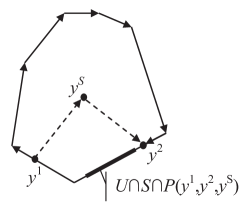
Fig. 2: Intersection of a face $S$ with the plane $P(y^{1},y^{S},y^{2})$ when $U\cap ri(S)=\emptyset$ (Lemma 5, case 2). In this intersection, $U\cap S\subset r\partial(S)$ belongs to one side of the polygon (the bold segment). The dashed lines with arrows represent the 3-vertex polygonal chain $[y^{1},y^{S},y^{2}]$. There exists a path from $y^{1}$ to $y^{2}$ along the boundary of the polygon. In Fig., this is the polygonal chain that follows the solid lines with arrows.

So, for any closed face $S\subset D$ with $\dim S=j\geq 2$ and a continuous path $\psi:[0,1]\to(D_{j}\setminus U)$ that connects the vertices $v,v^{\prime}$ of $D$ ($\psi(0)=v$, $\psi(1)=v^{\prime}$) we construct a continuous path $\psi_{S}:[0,1]\to(D_{j}\setminus U)$ that connects the same vertices, does not intersect $ri(S)$ and takes no new values outside $S$, $\psi_{S}([0,1])\setminus S\subseteq\psi([0,1])\setminus S$.

Let us order the faces $S\subseteq D$ with $\dim S\geq 2$ in such a way that $\dim S_{i}\geq\dim S_{j}$ for $i<j$: $D=S_{0},S_{1},\ldots,S_{\ell}$. Let us start from a given path $\varphi:[0,1]\to D\setminus U$ that connects the vertices $v$ and $v^{\prime}$ and let us apply sequentially the described procedure:

$$\theta=(\ldots(((\varphi_{S_{0}})_{S_{1}})_{S_{2}})\ldots)_{S_{\ell}}\,.$$

By the construction, this path $\theta$ does not intersect any relative interior $ri(S_{k})$ ($k=0,1,\ldots,\ell$). Therefore, the image of $\theta$ belongs to $D_{1}$, $\theta:[0,1]\to(D_{1}\setminus U)$. It can be transformed into a simple path in $D_{1}\setminus U$ by deletion of all loops (if they exist). This simple path (without self-intersections) is just the sequence of edges we are looking for. ∎

Lemmas 4, 5 allow us to describe the connected components of the $d$-dimensional set $D\setminus U$ through the connected components of the one-dimensional continuum $D_{1}\setminus U$.

Proposition 6.

Let $W_{1},\ldots,W_{q}$ be all the path-connected components of $D\setminus U$. Then $W_{i}\cap D_{0}\neq\emptyset$ for all $i=1,\ldots,q$, the continuum $D_{1}\setminus U$ has $q$ path-connected components and $W_{i}\cap D_{1}$ are these components.

Proof.

Due to Lemma 4, each path-connected component of $D\setminus U$ includes at least one vertex of $D$. According to Lemma 5, if two vertices of $D$ belong to one path-connected component of $D\setminus U$ then they belong to one path-connected component of $D_{1}\setminus U$. The reverse statement is obvious, because $D_{1}\subset D$ and a continuous path in $D_{1}$ is a continuous path in $D$. ∎

We can study connected components of a simpler, discrete object, the graph $\widetilde{D_{1}}$. The path-connected components of $D\setminus U$ correspond to the connected components of the graph $\widetilde{D_{1}}\setminus U$. (This graph is produced from $\widetilde{D_{1}}$ by deletion all the vertices that belong to $U_{0}$ and all the edges that belong to $U_{1}$).

Proposition 7.

Let $W_{1},\ldots,W_{q}$ be all the path-connected components of $D\setminus U$. Then the graph $\widetilde{D_{1}}\setminus U$ has exactly $q$ connected components and each set $W_{i}\cap D_{0}$ is the set of the vertices of $D$ of one connected component of $\widetilde{D_{1}}\setminus U$.

Proof.

Indeed, every path between vertices in $D_{1}$ includes a path that connects these vertices and is the sequence of edges. (To prove this statement we just have to delete all loops in a given path.) Therefore, the vertices $v_{1},v_{2}$ belong to one connected component of $\widetilde{D_{1}}\setminus U$ if and only if they belong to one path-connected component of $D_{1}\setminus U$. The rest of the proof follows from Proposition 6. ∎

We proved that the path-connected components of $D\setminus U$ are in one-to-one correspondence with the components of the graph $\widetilde{D_{1}}\setminus U$ (the correspondent components have the same sets of vertices). In applications, we will meet the following problem. Let a point $x\in D\setminus U$ be given. Find the path-connected component of $D\setminus U$ which includes this point. There are two basic ways to find this component. Assume that we know the connected components of $\widetilde{D_{1}}\setminus U$. First, we can examine the segments $[x,v]$ for all vertices $v$ of $D$. At least one of them does not intersect $U$ (Lemma 4). Let it be $[x,v_{0}]$. We can find the connected component $\widetilde{D_{1}}\setminus U$ that contains $v_{0}$. The point $x$ belongs to the correspondent path-connected component of $D\setminus U$. This approach exploits the $V$-description of the polyhedron $D$. The work necessary for this method is proportional to the number of vertices of $D$.

Another method is based on projection on the faces of $D$. Let $x\in ri(D)$. We can take any point $y^{0}\in D\setminus U$ and find the unique $\lambda_{1}>1$ such that $x^{1}=y_{0}+\lambda_{1}(x-y^{0})\in r\partial(D)$. Let $x^{1}\in ri(S_{1})$, where $S_{1}$ is a face of $D$. If $S_{1}\cap U=\emptyset$ then we can take any vertex $v_{0}\in S_{1}$ and find the connected component $\widetilde{D_{1}}\setminus U$ that contains $v_{0}$. This component gives us the answer. If $S_{1}\cap U\neq\emptyset$ then we can take any $y^{1}\in S_{1}\cap U$ and find the unique $\lambda_{2}>1$ such that $x^{2}=y^{1}+\lambda_{2}(x^{1}-y^{1})\in r\partial(S)$. This $x^{2}$ belongs to the relative boundary of the face $S_{1}$. If $x^{2}$ is not a vertex then it belongs to the relative interior of some face $S_{2}$, $\dim S_{2}>0$ and we have to continue. At each iteration, the dimension of faces decreases. After $d=\dim D$ iterations at most we will get the vertex $v$ we are looking for (see also Fig. 1) and find the connected component of $\widetilde{D_{1}}\setminus U$ which gives us the answer. Here we exploit the $H$-description of $D$.

2.2 Description of the connected components of $D\setminus U$ by inequalities

Let $W_{1},\ldots,W_{q}$ be the path-connected components of $D\setminus U$.

Proposition 8.

For any set of indices $I\subset\{1,\ldots,q\}$ the set

$$K_{I}=U\bigcup\left(\bigcup_{i\in I}W_{i}\right)$$

is convex.

Proof.

Let $y^{1},y^{2}\in K_{I}$. We have to prove that $[y^{1},y^{2}]\subset K_{I}$. Five different situations are possible:

1. $y^{1},y^{2}\in U$;

2. $y^{1}\in U,\,y^{2}\in W_{i}$, $i\in I$;

3. $y^{1},y^{2}\in W_{i}$, $i\in I$, $[y^{1},y^{2}]\cap U=\emptyset$;

4. $y^{1},y^{2}\in W_{i}$, $i\in I$, $[y^{1},y^{2}]\cap U\neq\emptyset$;

5. $y^{1}\in W_{i},\,y^{2}\in W_{j}$, $i,j\in I$, $i\neq j$.

We will systematically use two simple facts: (i) the convexity of $U$ implies that its intersection with any segment is a segment and (ii) if $x^{1}\in W_{i}$ and $x^{2}\in D\setminus W_{i}$ then the segment $[x^{1},x^{2}]$ intersects $U$ because $W_{i}$ is a path-connected component of $U$.

In case 1, $[y^{1},y^{2}]\subset U\subset K$ because convexity $U$.

In case 2, there exists such a point $y^{3}\in(y^{1},y^{2})$ that $[y^{1},y^{3})\subseteq U\cap[y^{1},y^{2}]\subseteq[y^{1},y^{3}]$. The segment $(y^{3},y^{2}]$ cannot include any point $x\in D\setminus W_{i}$ because it does not include any point from $U$. Therefore, in this case $(y^{3},y^{2}]\subset W_{i}\subset K$ and $y^{3}\in K$ because it belongs either to $U$ or to $W_{i}$.

In case 3, $[y^{1},y^{2}]\subset W_{i}\subset K$ because $W_{i}$ is a path-connected component of $D\setminus U$ and $[y^{1},y^{2}]\cap U=\emptyset$.

In case 4, $[y^{1},y^{2}]\cap U$ is a segment $L$ with the ends $x^{1},x^{2}$. It may be $[x^{1},x^{2}]$ ($y^{1}<x^{1}\leq x^{2}<y^{2}$), $(x^{1},x^{2}]$ ($y^{1}\leq x^{1}<x^{2}<y^{2}$), $[x^{1},x^{2})$ ($y^{1}<x^{1}<x^{2}\leq y^{2}$), or $(x^{1},x^{2})$ ($y^{1}\leq x^{1}<x^{2}\leq y^{2}$). This segment cuts $[y^{1},y^{2}]$ in three segments: $[y^{1},y^{2}]=L_{1}\cup L\cup L_{2}$, $L_{1}$ includes $y^{1}$ and $L_{2}$ includes $y^{2}$. Therefore, $L_{1}\subset W_{i}$, $L\subset U$ and $L_{2}\subset W_{i}$ because $W_{i}$ is a path-connected component of $D\setminus U$ and $U$ is convex. So, $[y^{1},y^{2}]\subset K$.

In case 5, $[y^{1},y^{2}]\cap U$ is also a segment $L$ with the ends $x^{1},x^{2}$. It may be $[x^{1},x^{2}]$ ($y^{1}<x^{1}\leq x^{2}<y^{2}$), $(x^{1},x^{2}]$ ($y^{1}\leq x^{1}<x^{2}<y^{2}$), $[x^{1},x^{2})$ ($y^{1}<x^{1}<x^{2}\leq y^{2}$), or $(x^{1},x^{2})$ ($y^{1}\leq x^{1}<x^{2}\leq y^{2}$). This segment cuts $[y^{1},y^{2}]$ in three segments: $[y^{1},y^{2}]=L_{1}\cup L\cup L_{2}$, $L_{1}$ includes $y^{1}$ and $L_{2}$ includes $y^{2}$. Therefore, $L_{1}\subset W_{i}$, $L\subset U$ and $L_{2}\subset W_{j}$ because $W_{i,j}$ are path-connected components of $D\setminus U$ and $U$ is convex. So, $[y^{1},y^{2}]\subset K$. ∎

Typically, the set $U$ is represented by a set of inequalities, for example, $G(x)\leq g$. It may be useful to represent the path-connected components of $D\setminus U$ by inequalities. For this purpose, let us first construct a convex polyhedron $Q\subset U$ with the same number of path-connected components in $D\setminus Q$, $V_{1},\ldots,V_{q}$ and with inclusons $W_{i}\subset V_{i}$. We will construct $Q$ as a convex hull of a finite set. Let us select the edges $e$ of $D$ which intersect $U$ but the intersection $e\cap U$ does not include vertices of $D$. For every such edge we select one point $x_{e}\in e\cap U$. The set of these points is $Q_{1}$. By definition,

$$Q={\rm conv}(U_{0}\cup Q_{1})\,.$$ (7)

$Q$ is convex, hence, we can apply all the previous results about the components of $D\setminus U$ to the components of $D\setminus Q$.

Lemma 9.

The set $U_{0}\cup Q_{1}$ is the set of vertices of $Q$.

Proof.

A point $x\in U_{0}\cup Q_{1}$ is not a vertex of $Q={\rm conv}(U_{0}\cup Q_{1})$ if and only if it is a convex combination of other points from this set: there exist such $x_{1},\ldots,x_{k}\in U_{0}\cup Q_{1}$ and $\lambda_{1},\ldots,\lambda_{k}>0$ that $x_{i}\neq x$ for all $i=1,\ldots,k$ and

$$\sum_{i=1}^{k}\lambda_{i}=1\,,\;\;\sum_{i=1}^{k}\lambda_{i}x_{i}=x\,.$$

If $x\in U_{0}$ then this is impossible because $x$ is a vertex of $D$ and $U_{0}\cup Q_{1}\subset D$. If $x\in Q_{1}$ then it belongs to the relative interior of an edge of $D$ and, hence, may be a convex combination of points $D$ from this edge only. By construction, $U_{0}\cup Q_{1}$ may include only one internal point from an edge and in this case does not include a vertex from this edge. Therefore, all the points from $Q_{1}$ are vertices of $Q$. ∎

Lemma 10.

The set $D\setminus Q$ has $q$ path-connected components $V_{1},\ldots,V_{q}$ that may be enumerated in such a way that $W_{i}\subset V_{i}$ and $W_{i}=V_{i}\setminus U$.

Proof.

To prove this statement about the path-connected components, let us mention that $Q$ and $U$ include the same vertices of $D$, the set $U_{0}$, and cut the same edges of $D$. Graphs $\widetilde{D_{1}}\setminus Q$ and $\widetilde{D_{1}}\setminus U$ coincide. $Q\subset U$ because of the convexity of $U$ and definition of $Q$. To finalize the proof, we can apply Proposition 7. ∎

Proposition 11.

Let $I$ be any set of indices from $\{1,\ldots,q\}$.

$$Q\bigcup\left(\bigcup_{i\in I}V_{i}\right)={\rm conv}\left(U_{0}\bigcup Q_{1}\bigcup\left(\bigcup_{i\in I}\left(D_{0}\bigcap V_{i}\right)\right)\right)$$ (8)

Proof.

On the left hand side of (8) we see the union of $Q$ with the connected components $V_{i}$ ($i\in I$). On the right hand side there is a convex envelope of a finite set. This finite set consists of the vertices of $Q$, ($U_{0}\cup Q_{1}$) and the vertices of $D$ that belong to $V_{i}$ ($i\in I$). Let us denote by $R_{I}$ the right hand side of (8) and by $L_{I}$ the left hand side of (8).

$L_{I}$ is convex due to Proposition 8 applied to $Q$ and $V_{i}$. The inclusion $R_{I}\subseteq L_{I}$ is obvious because $L_{I}$ is convex and $R_{I}$ is defined as a convex hull of a subset of $L_{I}$. To prove the inverse inclusion, let us consider the path-connected components of $D\setminus R_{I}$. Sets $V_{j}$ ($j\notin I$) are the path-connected components of $D\setminus R_{I}$ because they are the path-connected components of $D\setminus Q$, $Q\subset R_{I}$ and $R_{I}\cap V_{j}=\emptyset$ for $j\notin I$. There exist no other path-connected components of $Q\subset R_{I}$ because all the vertices of $V_{i}$ ($i\in I$) belong to $R_{I}$ by construction, hence, $D_{0}\setminus R_{I}\subset\cup_{j\notin I}V_{j}$. Due to Lemma 4 every path-connected component of $D\subset R_{I}$ includes at least one vertex of $D$. Therefore, $V_{j}$ ($j\notin I$) are all the path-connected components of $D\setminus R_{I}$ and $D\setminus R_{I}=\cup_{j\notin I}V_{j}$. Finally, $R_{I}=D\setminus\cup_{j\notin I}V_{j}=Q\cup\left(\cup_{i\in I}V_{i}\right)=L_{I}$. ∎

According to Lemma 9, each path-connected component $W_{i}\subset D\setminus U$ can be represented in the form $W_{i}=V_{i}\setminus U$, where $V_{i}$ is a path-connected component of $D\setminus Q$. By construction, $Q\subset U$, hence

$$W_{i}=(Q\cup V_{i})\setminus U\,.$$ (9)

If $U$ is given by a system of inequalities then representations (8) and (9) give us the possibility to represent $W_{i}$ by inequalities. Indeed, the convex envelope of a finite set in (8) may be represented by a system of linear inequalities. If the sets $Q\cup V_{i}$ and $U$ in (9) are represented by inequalities then the difference between them is also represented by the system of inequalities.

The description of the path-connected component of $D\setminus U$ may be constructed by the following steps:

1. Construct the graph of the 1-skeleton of $D$, this is $\widetilde{D_{1}}$;

2. Find the vertices of $D$ that belong to $U$, this is the set $U_{0}$;

3. Find the edges of $D$ that intersect $U$, this is the set $U_{1}$.

4. Delete from $\widetilde{D_{1}}$ all the vertices from $U_{0}$ and the edges from $U_{1}$, this is the graph $\widetilde{D_{1}}\setminus U$;

5. Find all the connected components of $\widetilde{D_{1}}\setminus U$. Let the sets of vertices of these connected components be $V_{01},\ldots,V_{0q}$;

6. Select the edges $e$ of $D$ which intersect $U$ but the intersection $e\cap U$ does not include vertices of $D$. For every such an edge select one point $x_{e}\in e\cap U$. The set of these points is $Q_{1}$.

7. For every $i=1,\ldots,q$ describe the polyhedron $R_{i}={\rm conv}(U_{0}\cup Q_{1}\cup V_{0i})$;

8. There exists $q$ path-connected components of $D\setminus U$: $W_{i}=R_{i}\setminus U$.

Every step can be performed by known algorithms including algorithms for the solution of the double description problem [49, 14, 21] and the convex hull algorithms [55].

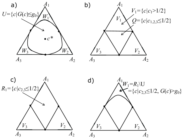
Fig. 3: Construction of the path-connected components $W_{i}$ of $D\setminus U$ for the simple example. (a) The balance simplex $D$, the set $U$ and the path-connected components $W_{i}$; (b) The polyhedron $Q={\rm conv}(U_{0}\cup Q_{1})$ (7) ($U_{0}=\emptyset$, $Q_{1}$ consists of the middles of the edges) and the connected components $V_{i}$ of $D\setminus Q$: $V_{i}=\{c\in D\,|\,c_{i}>1/2\}$; (c) The set $R_{1}={\rm conv}(U_{0}\cup Q_{1}\cup(D_{0}\cap V_{1}))$; (d) The connected components $W_{1}$ described by the inequalities (as $R_{1}\setminus U$ (8)).

Let us use the simple system of three reagents, $A_{1,2,3}$ (Fig. 1) to illustrate the main steps of the construction of the path-connected components. The polyhedron $D$ is here the 2D simplex (Fig. 1a). The plane ${\rm Aff}D$ is given by the balance equation $c_{1}+c_{2}+c_{3}=1$. We select $U=\{c\,|\,G(c)\leq g_{0}\}$ as an example of a convex set (Fig. 3a). It includes no vertices of $D$, hence, $U_{0}=\emptyset$. $U$ intersects each edge of $D$ in the middle point, hence, $U_{1}$ includes all the edges of $D$. The graph $\widetilde{D_{1}}\setminus U$ consists of three isolated vertices. Its connected components are these isolated vertices. $Q_{1}$ consists of three points, the middles of the edges $(1/2,1/2,0)$, $(1/2,0,1/2)$ and $(0,1/2,1/2)$ (in this example, the choice of these points is unambiguous, Fig. 3a).

The polyhedron $Q$ is a convex hull of these three points, that is the triangle given in ${\rm Aff}(D)$ by the system of three inequalities $c_{1,2,3}\leq 1/2$ (Fig. 3b). The connected components of $D\setminus Q$ are the triangles $V_{i}$ given in $D$ by the inequalities $c_{i}>1/2$. In the whole $\mathbb{R}^{3}$, these sets are given by the systems of an equation and inequalities:

$$V_{i}=\{c\,|\,c_{1,2,3}\geq 0,\,c_{1}+c_{2}+c_{3}=1,\,c_{i}>1/2\}\,.$$

The polyhedron $R_{i}$ is the convex hull of four points, the middles of the edges and the $i$th vertex (Fig. 3c). In $D$, $R_{i}$ is given by two linear inequalities, $c_{j}\leq 1/2,\,j\neq i$. In the whole $\mathbb{R}^{3}$, these inequalities should be supplemented by the equation and inequalities that describe $D$:

$$R_{i}=\{c\,|\,c_{1,2,3}\geq 0,\,c_{1}+c_{2}+c_{3}=1,\,c_{j}\leq 1/2\,(j\neq i)\}\,.$$

The path-connected components of $D\setminus U$, $W_{i}$ are described as $R_{i}\setminus U$ Fig. 3d): in $D$ we get $W_{i}=\{c\,|\,c_{j}\leq 1/2\,(j\neq i),\,G(c)>g_{0}\}$. In the whole $\mathbb{R}^{3}$,

$$W_{i}=\{c\,|\,c_{1,2,3}\geq 0,\,c_{1}+c_{2}+c_{3}=1,\,c_{j}\leq 1/2\,(j\neq i),\,G(c)>g_{0}\}\,.$$

$V_{i}$ are convex sets in this simple example, therefore, it is possible to simplify slightly the description of the components $W_{i}$ and to represent them as $V_{i}\setminus U$:

$$W_{i}=\{c\,|\,c_{1,2,3}\geq 0,\,c_{1}+c_{2}+c_{3}=1,\,c_{i}>1/2,\,G(c)>g_{0}\}\,$$

(or $W_{i}=\{c\,|\,c_{i}>1/2,\,G(c)>g_{0}\}$ in $D$).

In the general case (more components and balance conditions), the connected components $V_{i}$ may be non-convex, hence, description of these sets by the systems of linear equations and inequalities may be impossible. Nevertheless, there exists another version of the description of $W_{i}$ where a smaller polyhedron is used instead of $R_{i}$

Let $V_{0i}$ be the set of vertices of a connected component of the graph $\widetilde{D_{1}}\setminus U$. Let $E_{\rm out}(V_{0i})$ be the set of the outer edges of $V_{0i}$ in $\widetilde{D_{1}}$ i.e., this is the set of edges of $\widetilde{D_{1}}$ that connect vertices from $V_{0i}$ with vertices from $D_{0}\setminus V_{0i}$. For each $e\in E_{\rm out}(V_{0i})$ the corresponding edge $e\subset D_{1}$ intersects $U$ because $V_{0i}$ is the set of vertices of a connected component of the graph $\widetilde{D_{1}}\setminus U$.

Let us select a point $x_{e}\in U\cap e$ for each $e\in E_{\rm out}(V_{0i})$ (we use the same notations for the edges from $\widetilde{D_{1}}$ and the corresponding edges from ${D_{1}}$). Let us use the notation

$$Q_{0i}=\{x_{e}\,|\,e\in E_{\rm out}(V_{0i})\}\,.$$

Proposition 12.

The path-connected component $W_{i}$ of $D\setminus U$ allows the following description:

$$W_{i}={\rm conv}(Q_{0i}\cup V_{0i})\setminus U\,.$$

Proof.

The set $Q_{0i}\subset U$ and $V_{0i}$ is the set of vertices of a connected component of the graph $\widetilde{D_{1}}\setminus Q_{0i}$ by construction because $Q_{0i}$ cuts all the outer edges of $V_{0i}$ in $D_{1}$. The rest of the proof follows the proofs of Lemma 10 and Proposition 11. ∎

This proposition allows us to describe $W_{i}$ by the system of inequalities. For this purpose, we have to use a convex hull algorithm and describe the convex hull ${\rm conv}(Q_{0i}\cup V_{0i})$ by the system of linear inequalities and then add the inequality that describes the set $\setminus U$.

In the simple system (Fig. 3), the connected components of the graph $\widetilde{D_{1}}\setminus U$ are the isolated vertices. The set $Q_{0i}$ for the vertex $A_{i}$ consists of two middles of its incident edges. In Fig. 3b, the set ${\rm conv}(Q_{0i}\cup V_{0i})$ for $V_{0i}=\{A_{1}\}$ is the triangle $V_{1}$.

3 Thermodynamic tree

3.1 Problem statement

Let a real continuous function $G$ be given in the convex bounded polyhedron $D\subset\mathbb{R}^{n}$. We assume that $G$ is strictly convex in $D$, i.e. the set (the epigraph of $G$)

$${\rm epi}(G)=\{(x,g)\,|\,x\in D,\,g\geq G(x)\}\subset D\times(-\infty,\infty)$$

is convex and for any segment $[x,y]\subset D$ ($x\neq y$) $G$ is not constant on $[x,y]$. A strictly convex function on a bounded convex set has a unique minimizer. Let $x^{*}$ be the minimizer of $G$ in $D$ and let $g^{*}=G(x^{*})$ be the corresponding minimal value. The level set $S_{g}=\{x\in D\,|\,G(x)=g\}$ is closed and the sublevel set $U_{g}=\{x\in D\,|\,G(x)<g\}$ is open in $D$. The sets $S_{g}$ and $D\setminus U_{g}$ are compact and $S_{g}\subset D\setminus U_{g}$.

Let $x,y\in D$. According to Corollary 16 proven in the next subsection, an admissible path from $x$ to $y$ in $D$ exists if and only if $\pi(y)$ belongs to the ordered segment $[\pi(x^{*}),\pi(x)]$. Therefore, to describe constructively the relation $x\succsim y$ in $D$ we have to solve the following problems:

1. How to construct the thermodynamic tree $\mathcal{T}$?

2. How to find an image $\pi(x)$ of a state $x\in D$ on the thermodynamic tree $\mathcal{T}$?

3. How to describe by inequalities a preimage of an ordered segment of the thermodynamic tree, $\pi^{-1}([w,z])\subset D$ ($w,z\in\mathcal{T}$, $z\succsim w$)?

3.2 Coordinates on the thermodynamic tree

We get the following lemma directly from Definition 1. Let $x,y\in D$.

Lemma 13.

$x\sim y$ if and only if $G(x)=G(y)$ and $x$ and $y$ belong to the same path-connected component of $S_{g}$ with $g=G(x)$.

The path-connected components of $D\setminus U_{g}$ can be enumerated by the connected components of the graph $\widetilde{D_{1}}\setminus U_{g}$. The following lemma allows us to apply this result to the path-connected components of $S_{g}$.

Lemma 14.

Let $g>g^{*}$, $W_{1},\ldots,W_{q}$ be the path-connected components of $D\setminus U_{g}$ and let $\sigma_{1},\ldots,\sigma_{p}$ be the path-connected components of $S_{g}$. Then $q=p$ and $\sigma_{i}$ may be enumerated in such a way that $\sigma_{i}$ is the border of $W_{i}$ in $D$.

Proof.

$G$ is continuous in $D$, hence, if $G(x)>g$ then there exists a vicinity of $x$ in $D$ where $G(x)>g$. Therefore $G(y)=g$ for every boundary point $y$ of $D\setminus U_{g}$ in $D$ and $S_{g}$ is the boundary of $D\setminus U_{g}$ in $D$.

Let us define a projection $\theta_{g}:D\setminus U_{g}\to S_{g}$ by the conditions: $\theta_{g}(x)\in[x,x^{*}]$ and $G(\theta_{g}(x))=g$. By definition, the inequality $G(x)\geq g$ holds in $D\setminus U_{g}$. The function $f_{x}(\lambda)=G((1-\lambda)x^{*}+\lambda x)$ is strictly increasing, continuous and convex function of $\lambda\in[0,1]$, $f_{x}(0)=g^{*}<g$, $f_{x}(1)=G(x)\geq g$. The function $f_{x}(\lambda)$ depends continuously on $x\in D\setminus U_{g}$ in the uniform metrics. Therefore, the solution $\lambda_{x}$ to the equation $f_{x}(\lambda)=g$ on $[0,1]$ exists (the intermediate value theorem), is unique, and continuously depends on $x\in D\setminus U_{g}$. The projection $\theta_{g}$ is defined as $\theta_{g}(x)=(1-\lambda_{x})x^{*}+\lambda_{x}x$.

The fixed points of the projection $\theta_{g}$ are elements of $S_{g}$. The image of each path-connected component $W_{i}$ is a path-connected set. The preimage of every path-connected component $\sigma_{i}$ is also a path-connected set. Indeed, let $\theta_{g}(x)\in\sigma_{i}$ and $\theta_{g}(y)\in\sigma_{i}$. There exists a continuous path from $x$ to $y$ in $D\setminus U_{g}$. It may be composed from three paths: (i) from $x$ to $\theta_{g}(x)$ along the line segment $[x,\theta_{g}(x)]\subset[x,x^{*}]$ then a continuous path in $\sigma_{i}$ between $\theta_{g}(x)$ and $\theta_{g}(y)$ (it exists because $\sigma_{i}$ is a path-connected component of $S_{g}$ and it belongs to $D\setminus U_{g}$ because $S_{g}\subset D\setminus U_{g}$) and, finally, from $\theta_{g}(y)$ to $y$ along the line segment $[\theta_{g}(y),y]\subset[x^{*},y]$. Therefore, the image of a path-connected component $W_{i}$ is a path-connected components of $S_{g}$ that may be enumerated by the same index $i$, $\sigma_{i}$. This $\sigma_{i}$ is the border of $W_{i}$ in $D$. ∎

The equivalence class of $x\in D$ is defined as $[x]=\{y\in D\,|\,y\sim x\}$. Let $W(x)$ be a path-connected component of $D\setminus U_{g}$ ($g=G(x)$) for which $\theta_{g}(W(x))=[x]$. Due to Lemma 14, such a component exists and

$$W(x)=\{y\in D\,|\,y\succsim x\}\,.$$ (10)

Let us define a one-dimensional continuum $\mathcal{Y}$ that consists of the pairs $(g,M)$, where $g^{*}\leq g\leq g_{\max}$ and $M$ is a set of vertices of a connected component of $\widetilde{D_{1}}\setminus U_{g}$. For each $(g,M)$ the fundamental system of neighborhoods consists of the sets $V_{\rho}$ ($\rho>0$):

$$V_{\rho}=\{(g^{\prime},M^{\prime})\,|\,(g^{\prime},M^{\prime})\in\mathcal{Y},\,|g-g^{\prime}|<\rho,\,M^{\prime}\subseteq M\}\,.$$ (11)

Let us define the partial order on $\mathcal{Y}$:

$$(g,M)\succsim(g^{\prime},M^{\prime})\mbox{ if }g\geq g^{\prime}\mbox{ and }M\subseteq M^{\prime}\,.$$

Let us introduce the mapping $\omega:D\to\mathcal{Y}$:

$$\omega(x)=(G(x),W(x)\cap D_{0})\,.$$

Theorem 15.

There exists a homeomorphism between $\mathcal{Y}$ and $\mathcal{T}$ that preserves the partial order and makes the following diagram commutative:

Proof.

According to Lemmas 14, 10 and Proposition 7, $\omega$ maps the equivalent points $x$ to the same pair $(g,M)$ and the non-equivalent points to different pairs $(g,M)$. For any $x,y\in D$, $x\succsim y$ if and only if $\omega(x)\succsim\omega(y)$.

The fundamental system of neighborhoods in $Y$ may be defined using this partial order. Let us say that $(g,M)$ is compatible to $(g^{\prime},M^{\prime})$ if $(g^{\prime},M^{\prime})\succsim(g,M)$ or $(g,M)\succsim(g^{\prime},M^{\prime})\}$. Then for $\rho>0$

$$V_{\rho}=\{(g^{\prime},M^{\prime})\in\mathcal{Y}\,|\,|\gamma-\gamma^{\prime}|<\rho\mbox{ and }(g^{\prime},M^{\prime})\mbox{ is compatible to }(g,M)\}\,.$$

For sufficiently small $\rho$ this definition coincides with (11).

So, by the definition of $\mathcal{T}$ as a quotient space $D/\sim$, $\mathcal{Y}$ has the same partial order and topology as $\mathcal{T}$. The isomorphism between $\mathcal{Y}$ and $\mathcal{T}$ establishes one-to-one correspondence between the $\pi$-image of the equivalence class $[x]$, $\pi([x])$, and the $\omega$-image of the same class, $\omega([x])$. ∎

$\mathcal{Y}$ can be considered as a coordinate system on $\mathcal{T}$. Each point is presented as a pair $(g,M)$ where $g^{*}\leq g\leq g_{\max}$ and $M$ is a set of vertices of a connected component of $\widetilde{D_{1}}\setminus U_{g}$. The map $\omega$ is the coordinate representation of the canonical projection $\pi:D\to\mathcal{T}$. Now, let us use this coordinate system and the proof of Theorem 15 to obtain the following corollary.

Corollary 16.

An admissible path from $x$ to $y$ in $D$ exists if and only if

$$\pi(y)\in[\pi(x^{*}),\pi(x)]\,.$$

Proof.

Let there exist an admissible path from $x$ to $y$ in $D$, $\varphi:[0,1]\to D$. Then $\pi(x)\succsim\pi(y)$ in $\mathcal{T}$. Let $\pi(x)=(G(x),M)$ in coordinates $\mathcal{Y}$. For any $v\in M$, $\pi(y)\in[\pi(x^{*}),\pi(v)]$ and $\pi(x)\in[\pi(x^{*}),\pi(v)]$.

Assume now that $\pi(y)\in[\pi(x^{*}),\pi(x)]$ and $\pi(x)=(G(x),M)$. Then the admissible path from $x$ to $y$ in $D$ can be constructed as follows. Let $v\in M$ be a vertex of $D$. $G(v)\geq G(x)$ for each $v\in M$. The straight line segment $[x^{*},v]$ includes a point $x_{1}$ with $G(x_{1})=G(x)$ and $y_{1}$ with $G(y_{1})=G(y)$. Coordinates of $\pi(x_{1})$ and $\pi(x)$ in $\mathcal{Y}$ coincide as well as coordinates of $\pi(y_{1})$ and $\pi(y)$. Therefore, $x\sim x_{1}$ and $y\sim y_{1}$. The admissible path from $x$ to $y$ in $D$ can be constructed as a sequence of three paths: first, a continuous path from $x$ to $x_{1}$ inside the path-connected component of $S_{G(x)}$ (Lemma 13), then from $x_{1}$ to $y_{1}$ along a straight line and after that a continuous path from $y_{1}$ to $y$ inside the path-connected component of $S_{G(y)}$. ∎

To describe the space $\mathcal{T}$ in coordinate representation $\mathcal{Y}$, it is necessary to find the connected components of the graph $\widetilde{D_{1}}\setminus U_{g}$ for each $g$. First of all, this function,

$$g\mapsto\mbox{ the set of connected components of }\widetilde{D_{1}}\setminus U_{g}\,,$$

is piecewise constant. Secondly, we do not need to solve at each point the computationally heavy problem of the construction of the connected components of the graph $\widetilde{D_{1}}\setminus U_{g}$ “from scratch”. The problem of the parametric analysis of these components as functions of $g$ appears to be much cheaper. Let us present a solution of this problem. At the same time, this is a method for the construction of the thermodynamic tree in coordinates $(g,M)$.

The coordinate system $\mathcal{Y}$ allows us to describe the tree structure of the continuum $\mathcal{T}$. This structure includes a root, $(g^{*},D_{0})$, edges, branching points and leaves.

Let $M$ be a connected component of $\widetilde{D_{1}}\setminus U_{g}$ for some $g$, $g^{*}<g<g_{\max}$. If $M\subsetneqq D_{0}$ then the set of all points $(g,M)\in\mathcal{T}$ has for a given $M$ the form $(\underline{a}_{M},\overline{a}_{M}]\times M$, $\underline{a}_{M}<\overline{a}_{M}$. We call this set an edge of $\mathcal{T}$.

If $M$ includes all the vertices of $D$ ($M=D_{0}$) then the set of all points $(g,M)\in\mathcal{T}$ has the form $[g^{*},\overline{a}_{D_{0}}]\times D_{0}$. This may be either an edge (if $\overline{a}_{D_{0}}>g^{*}$) or just a root, $\{(g^{*},D_{0})\}$, (this is possible in 1D systems).

Let us define the numbers $\underline{a}_{M}=\inf\{g\,|\,(g,M)\in\mathcal{T}\}$. Let us introduce the set of outer edges of $M$ in $\widetilde{D_{1}}$, $E_{\rm out}(M)$. This is the set of edges of $\widetilde{D_{1}}$ that connect vertices from $M$ with vertices from $D_{0}\setminus M$. We keep the same notation, $E_{\rm out}(M)$, for the set of the corresponding edges of $D$.

$$\underline{a}_{M}=\max_{e\in E_{out}(M)}\min\{G(x)\,|\,x\in e\}\,.$$ (12)

This number, $\underline{a}_{M}$, is the “cutting value” of $G$ for $M$. It cuts $M$ from the other vertices of $\widetilde{D_{1}}$ in the following sense: if we delete from $\widetilde{D_{1}}$ all the edges $e$ with the label values $<\underline{a}_{M}$ then $M$ will remain attached to some vertices from $D_{0}\setminus M$. If we delete the edges with the label values $\leq\underline{a}_{M}$ then $M$ becomes disconnected from $D_{0}\setminus M$. There is the only connected component of $\widetilde{D_{1}}\setminus U_{\underline{a}_{M}}$ that includes $M$, $M^{\prime}\supsetneqq M$. The pair $(\underline{a}_{M},M^{\prime})\in\mathcal{T}$ is a branching point of $\mathcal{T}$. The edge $(\underline{a}_{M},\overline{a}_{M}]\times M$ connects two vertices, the upper vertex $(\overline{a}_{M},M)$ and the lower vertex, $(\underline{a}_{M},M^{\prime})$.

If $M$ consists of one vertex, $M=\{v\}$, then the point $(G(v),\{v\})$ is a leaf of $\mathcal{T}$.

3.3 Construction of the thermodynamic tree

To construct the tree of $G$ in $D$ we need the graph $\widetilde{D_{1}}$ of the 1-skeleton of the polyhedron $D$. Elements of $\widetilde{D_{1}}$ should be labeled by the values of $G$. Each vertex $v$ is labeled by the value $\gamma_{v}=G(v)$ and each edge $e=[v,w]$ is labeled by the minimal value of $G$ on the segment $[v,w]\subset D$, $g_{e}=\min_{[v,w]}G(x)$. We need also the minimal value $g^{*}=\min_{D}\{G(x)\}$ because the root of the tree is $(g^{*},D_{0})$.

The strictly convex function $G$ achieves its local maxima in $D$ only in vertices. The vertex $v$ is a (local) maximizer of $g$ if $g_{e}<\gamma_{v}$ for each edge $e$ that includes $v$. The leaves of the thermodynamic tree are pairs $(\gamma_{v},\{v\})$ for the vertices that are the local maximizers of $G$.

As a preliminary step of the construction, we arrange and enumerate the labels of the elements of $\widetilde{D_{1}}$, the vertices and edges, in descending order. Let there exist $l$ different label values: $g_{\max}=a_{1}>a_{2}>\ldots>a_{l}$. Each $a_{k}$ is a value $\gamma_{v}=G(v)$ at a vertex $v\in D_{0}$ or the minimum of $G$ on an edge $e\subset D_{1}$ (or both). Let $A_{i}$ be the set of vertices $v\in D_{0}$ with $\gamma_{v}=a_{i}$ and let $E_{i}$ be the set of edges of $D_{1}$ with $g_{e}=a_{i}$ ($i=1,\ldots,l$).

Let us construct the connected components of the graph $\widetilde{D_{1}}\setminus U_{g}$ starting from $a_{1}=g_{\max}$. The function $G$ is strictly convex, hence, $a_{1}=\gamma_{v}$ for a set of vertices $A_{1}\subset D_{0}$ but it is impossible that $a_{1}=g_{e}$ for an edge $e$, hence, $E_{1}=\emptyset$.

The set of connected components of $\widetilde{D_{1}}\setminus U_{g}$ is the same for all $g\in(a_{i+1},a_{i}]$. For an interval $(a_{2},a_{1}]$ the connected components of $\widetilde{D_{1}}\setminus U_{g}$ are the one-element sets $\{v\}$ for $v\in A_{1}$.

For $g\in[g^{*},a_{l}]$ the graph $\widetilde{D_{1}}\setminus U_{g}$ includes all the vertices and edges of $\widetilde{D_{1}}$ and, hence, it is connected for this segment. Let us take, formally, $a_{l+1}=g^{*}$.

Let $\mathcal{L}_{i}=\{M^{i}_{1},\ldots,M_{k_{i}}^{i}\}$ be the set of the connected components of $\widetilde{D_{1}}\setminus U_{g}$ for $g\in(a_{i},a_{i-1}]$ ($i=1,\ldots,l$). Each connected component is represented by the set of its vertices $M^{i}_{j}$. Let us describe the recursive procedure for construction of $\mathcal{L}_{i}$:

1. Let us take formally $\mathcal{L}_{0}=\emptyset$.

2. Assume that $\mathcal{L}_{i-1}$ is given and $i\leq l$. Let us find the set $\mathcal{L}_{i}$ of connected components of $\widetilde{D_{1}}\setminus U_{g}$ for $g=a_{i}$ (and, therefore, for $g\in(a_{i+1},a_{i}]$).

   • Add the one-element sets $\{v\}$ for all $v\in A_{i}$ to the set

     $$\mathcal{L}_{i-1}=\{M^{i-1}_{1},\ldots,M_{k_{i-1}}^{i-1}\}\,.$$

     Denote this auxiliary set of sets as $\widetilde{L}_{i,0}=\{M_{1},\ldots,M_{q}\}$, where $q=k_{i-1}+|A_{i}|$.

   • Enumerate the edges from $E_{i}$ in an arbitrary order: $e_{1},\ldots,e_{|E_{i}|}$. For each $k=0,\ldots,|E_{i}|$, create recursively an auxiliary set of sets $\widetilde{L}_{i,k}$ by the union of some of elements of $\widetilde{L}_{k-1}$: Let $\widetilde{L}_{i,k-1}$ be given and $e_{k}$ connects the vertices $v$ and $v^{\prime}$. If $v$ and $v^{\prime}$ belong to the same element of $\widetilde{L}_{i,k-1}$ then $\widetilde{L}_{i,k}=\widetilde{L}_{i,k-1}$. If $v$ and $v^{\prime}$ belong to the different elements of $\widetilde{L}_{i,k-1}$, $M$ and $M^{\prime}$, then $\widetilde{L}_{i,k}$ is produced from $\widetilde{L}_{i,k-1}$ by the union of $M$ and $M^{\prime}$:

     $$\widetilde{L}_{i,k}=(\widetilde{L}_{i,k-1}\setminus\{M\}\setminus\{M^{\prime}\})\cup\{M\cup M^{\prime}\}$$

     (we delete two elements, $M$ and $M^{\prime}$, from $\widetilde{L}_{i,k-1}$ and add a new element $M\cup M^{\prime}$).

   The set $\mathcal{L}_{i}$ of connected components of $\widetilde{D_{1}}\setminus U_{g}$ for $g=a_{i}$ is $\mathcal{L}_{i}=\widetilde{L}_{i,|E_{i}|}$.

Generically, all the labels of the graph $\widetilde{D_{1}}$ vertices and edges are different and the sets $E_{i}$ and $A_{i}$ include not more than one element. Moreover, for each $i$ either $E_{i}$ or $A_{i}$ is generically empty and the description of the recursive procedure may be simplified for the generic case:

1. Let us take formally $\mathcal{L}_{0}=\emptyset$.

2. Assume that $\mathcal{L}_{i-1}$ is given and $i\leq l$.

   • If $a_{i}$ is a label of a vertex $v$, $a_{i}=\gamma_{v}$, then add the one-element set $\{v\}$ to the set $\mathcal{L}_{i-1}$: $\mathcal{L}_{i}=\mathcal{L}_{i-1}\cup\{\{v\}\}$.

   • Let $a_{i}$ be a label of an edge $e=[v,v^{\prime}]$. If $v$ and $v^{\prime}$ belong to the same element of $\mathcal{L}_{i-1}$ then $\mathcal{L}_{i}=\mathcal{L}_{i-1}$. If $v$ and $v^{\prime}$ belong to the different elements of $\mathcal{L}_{i-1}$, $M$ and $M^{\prime}$, then $\mathcal{L}_{i}$ is produced from $\mathcal{L}_{i-1}$ by the union of $M$ and $M^{\prime}$ (delete elements $M$ and $M^{\prime}$ and add an element $M\cup M^{\prime}$).

The described procedure gives us the sets of connected components of $\widetilde{D_{1}}\setminus U_{g}$ for all $g$ and, therefore, we get the tree $\mathcal{T}$. The descent from the higher values of $G$ allows us to avoid the solution of the computationally more expensive problem of the calculation of the connected components of a graph at any level of $G$.

3.4 The problem of attainable sets

In this section, we demonstrate how to solve the problem of attainable sets. For given $x\in D$ (an initial state) we describe the attainable set

$$Att(x)=\{y\in D\,|\,x\succsim y\}$$

by a system of inequalities. Let the tree $\mathcal{T}$ of $G$ in $D$ be given and let all the pairs $(g,M)\in\mathcal{T}$ be described. We also use the notation $Att(z)$ for sets attainable in $\mathcal{T}$ from $z\in\mathcal{T}$.

First of all, let us describe the preimage of a point $(g,M)\in\mathcal{T}$ in $D$. It can be described by the equation $G(x)=g$ and a set of linear inequalities. For each edge $e$ we select a minimizer of $G$ on $e$, $x_{e}={\rm argmin}\{G(x)\,|\,x\in e\}$ (we use the same notations for the elements of the graph $\widetilde{D_{1}}$ and of the continuum $D_{1}$). Let

$$Q_{M}=\{x_{e}\,|\,e\in E_{\rm out}(M)\}\,.$$

In particular, $\underline{a}_{M}=\max\{G(x)\,|\,x\in Q_{M}\}$.

The following Proposition is a direct consequence of Proposition 12.

Proposition 17.

The preimage of $(g,M)$ in $D$ is a set

$$\pi^{-1}(g,M)=\{x\in{\rm conv}(Q_{M}\cup M)\,|\,G(x)=g\}\,.$$ (13)

The sets $M$ and $Q_{M}$ in (13) do not depend on the specific value of $g$. It is sufficient that the point $(g,M)\in\mathcal{T}$ exists.

Let us consider the second projection of $\mathcal{T}$, i.e., the set of all connected components of the graph $\widetilde{D_{1}}\setminus U_{g}$ for all $g$. For a connected component $M$, the lower chain of connected components is a sequence $M=M_{1}\subsetneqq M_{2}\subsetneqq\ldots\subsetneqq M_{k}$. (“Lower” here means the descent in the natural order in $\mathcal{T}$, $\succsim$.) For a given initial element $M=M_{1}$ the maximal lower chain of $M$ is the lower chain of $M$ that cannot be extended by adding new elements. By construction of connected components, the maximal lower chain of $M$ is unique for each initial element $M$. In the maximal lower chain $\underline{a}_{M_{i}}=\overline{a}_{M_{i+1}}$.

For each set of values $H\subset(\underline{a}_{M},\overline{a}_{M}]$ the preimage of the set $H\times M\subset\mathcal{T}$ is given by (13) as

$$\pi^{-1}(H\times M)=\{x\in{\rm conv}(Q_{M}\cup M)\,|\,G(x)\in H\}\,.$$ (14)

We describe the set $Att(x)$ for $x\in D$ by the following procedures: (i) find the projection $\pi(x)$ of $x$ onto $\mathcal{T}$, (ii) find the attainable set in $\mathcal{T}$ from $\pi(x)$, $Att(\pi(x))$, and (iii) find the preimage of this set in $D$:

$$Att(x)=\pi^{-1}(Att(\pi(x)))\,.$$ (15)

The attainable set $Att(g,M)$ in $\mathcal{T}$ from $(g,M)\in\mathcal{T}$ is constructed as a union of edges and its parts. Let $M=M_{1}\subsetneqq M_{2}\subsetneqq\ldots\subsetneqq M_{k}=D_{0}$ be the maximal lower chain of $M$. Then

$$\begin{split}Att(g,M)=&(\underline{a}_{1},g]\times M_{1}\cup(\underline{a}_{2},\underline{a}_{1}]\times M_{2}\cup\ldots\\ &\cup(\underline{a}_{k-1},\underline{a}_{k-2}]\times M_{k-1}\cup[\underline{a}_{k},\underline{a}_{k-1}]\times M_{k}\,,\end{split}$$ (16)

where $\underline{a}_{i}=\underline{a}_{M_{i}}$.

To find the preimage of $Att(g,M)$ in $D$ we have to apply formula (14) to each term of (16). In Sec. 1.3 we demonstrated how to find $\pi(x)$. Therefore, each step of the solution of the problem of attainable set (15) is presented.

4 Chemical thermodynamics: examples

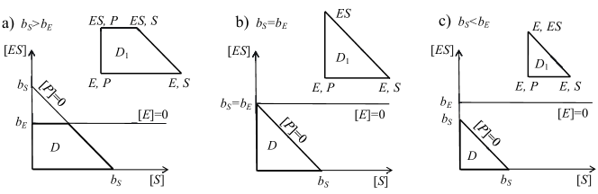
Fig. 4: The balance polygon $D$ on the plane with coordinates $[S]$ and $[ES]$ for the four–component enzyme–substrate system $S$, $E$, $ES$ $P$ with two balance conditions, $b_{S}=[S]+[ES]+[P]={\rm const}$ and $b_{E}=[E]+[ES]={\rm const}$.

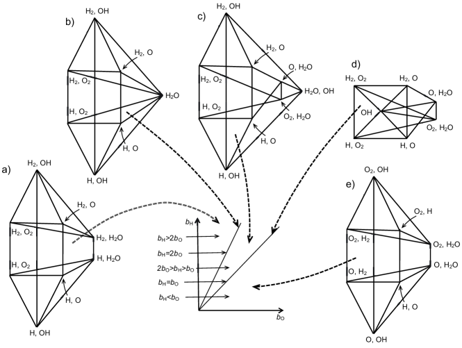
Fig. 5: The graph $\widetilde{D_{1}}(b)$ of the one-skeleton of the balance polyhedron for the six-component system, ${\rm H}_{2}$, ${\rm O}_{2}$, ${\rm H}$, ${\rm O}$, ${\rm H}_{2}{\rm O}$, ${\rm OH}$, as a piece-wise constant function of $b=(b_{\rm H},b_{\rm O})$. For each vertex the components are indicated which have non-zero concentrations at this vertex.

4.1 Skeletons of the balance polyhedra

In chemical thermodynamics and kinetics, the variable $N_{i}$ is the amount of the $i$th component in the system. The balance polyhedron $D$ is described by the positivity conditions $N_{i}\geq 0$ and the balance conditions (1) $b_{i}(N)={\rm const}$ ($i=1,\ldots,m$). Under the isochoric (the constant volume) conditions, the concentrations $c_{i}$ also satisfy the balance conditions and we can construct the balance polyhedron for concentrations. Sometimes, the balance polyhedron is called the reaction simplex with some abuse of language because it is not obligatory a simplex when the number $m$ of the independent balance conditions is greater than one.

The graph $\widetilde{D_{1}}$ depends on the values of the balance functionals $b_{i}=b_{i}(N)=\sum_{j=1}^{n}a_{i}^{j}N_{j}$. For the positive vectors $N$, the vectors $b$ with coordinates $b_{i}=b_{i}(N)$ form a convex polyhedral cone in $\mathbb{R}^{m}$. Let us denote this cone by $\Lambda$. $\widetilde{D_{1}}(b)$ is a piece-wise constant function on $\Lambda$. Sets with various constant values of this function are cones. They form a partition of $\Lambda$. Analysis of this partition and the corresponding values of $\widetilde{D_{1}}$ can be done by the tools of linear programming [26]. Let us represent several examples.

In the first example, the reaction system consists of four components: the substrate $S$, the enzyme $E$, the enzyme-substrate complex $ES$ and the product $P$. we consider the system under constant volume. We denote the concentrations by $[S]$, $[E]$, $[ES]$ and $[P]$. There are two balance conditions: $b_{S}=[S]+[ES]+[P]={\rm const}$ and $b_{E}=[E]+[ES]={\rm const}$.

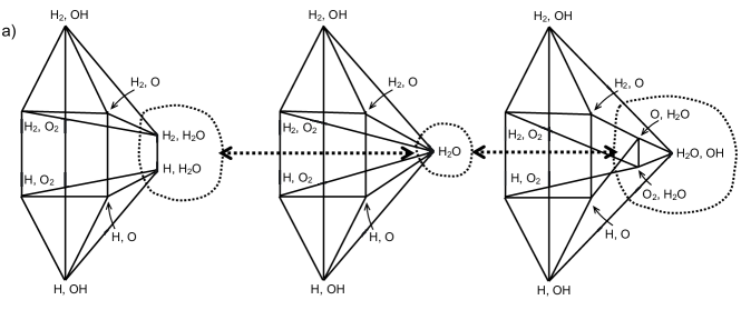
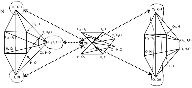
Fig. 6: Transformations of the graph $\widetilde{D_{1}}(b)$ with changes of the relation between $b_{\rm H}$ and $b_{\rm O}$: (a) transition from the regular case $b_{\rm H}>2b_{\rm O}$ to the regular case $2b_{\rm O}>b_{\rm H}>b_{\rm O}$ through the singular case $b_{\rm H}=2b_{\rm O}$, (b) transition from the regular case $2b_{\rm O}>b_{\rm H}>b_{\rm O}$ to the regular case $b_{\rm H}<b_{\rm O}$ through the singular case $b_{\rm H}=b_{\rm O}$.

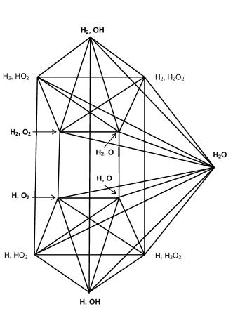
Fig. 7: The graph $\widetilde{D_{1}}$ for the eight-component system, ${\rm H}_{2}$, ${\rm O}_{2}$, ${\rm H}$, ${\rm O}$, ${\rm H}_{2}{\rm O}$, ${\rm OH}$, ${\rm H}_{2}{\rm O}_{2}$, ${\rm H}{\rm O}_{2}$ for the stoichiometric mixture, $b_{\rm H}=2b_{\rm O}$. The vertices that correspond also to the six-component mixture are distinguished by bold font.

For $b_{S}>b_{E}$ the polyhedron (here the polygon) $D$ is a trapezium (Fig. 4a). Each vertex corresponds to two components that have non-zero concentrations in this vertex. For $b_{S}>b_{E}$ there are four such pairs, $(ES,P)$, $(ES,S)$, $(E,P)$ and $(E,S)$. For two pairs there are no vertices: for $(S,P)$ the value $b_{E}$ is zero and for $(ES,E)$ it should be $b_{S}<b_{E}$. When $b_{S}=b_{E}$, two vertices, $(ES,P)$ and $(ES,S)$, transform into one vertex with one non-zero component, $ES$, an the polygon $D$ becomes a triangle (Fig. 4b). When $b_{S}<b_{E}$ then $D$ is also a triangle and a vertex $ES$ transforms in this case into $(ES,E)$ (Fig. 4c).

For the second example, we select a system with six components and two balance conditions: ${\rm H}_{2}$, ${\rm O}_{2}$, ${\rm H}$, ${\rm O}$, ${\rm H}_{2}{\rm O}$, ${\rm OH}$;

$$\begin{split}&b_{\rm H}=2N_{\rm H_{2}}+N_{\rm H}+2N_{\rm H_{2}O}+N_{\rm OH}\,,\\ &b_{\rm O}=2N_{\rm O_{2}}+N_{\rm O}+N_{\rm H_{2}O}+N_{\rm OH}\,.\end{split}$$

The cone $\Lambda$ is a positive quadrant on the plane with the coordinates $b_{\rm H},b_{\rm O}$. The graph $\widetilde{D_{1}}(b)$ is constant in the following cones in $\Lambda$ ($b_{\rm H},b_{\rm O}>0$): (a) $b_{\rm H}>2b_{\rm O}$, (b) $b_{\rm H}=2b_{\rm O}$, (c) $2b_{\rm O}>b_{\rm H}>b_{\rm O}$, (d) $b_{\rm H}=b_{\rm O}$ and (e) $b_{\rm H}<b_{\rm O}$ (Fig. 5).

The cases (a) $b_{\rm H}>2b_{\rm O}$, (c) $2b_{\rm O}>b_{\rm H}>b_{\rm O}$, and (e) $b_{\rm H}<b_{\rm O}$ (Fig. 5) are regular: there are two independent balance conditions and for each vertex there are exactly two components with non-zero concentration. In case (a) ($b_{\rm H}>2b_{\rm O}$), if $b_{\rm H}\to 2b_{\rm O}$ then two regular vertices, ${\rm H}_{2},\,{\rm H}_{2}{\rm O}$ and ${\rm H},\,{\rm H}_{2}{\rm O}$, join in one vertex (case (b)) with only one non-zero concentration, ${\rm H}_{2}{\rm O}$ (Fig. 6a). This vertex explodes in three vertices ${\rm O},\,{\rm H}_{2}{\rm O}$; ${\rm O}_{2},\,{\rm H}_{2}{\rm O}$ and ${\rm H}_{2}{\rm O},\,{\rm OH}$, when $b_{\rm H}$ becomes smaller than $2b_{\rm O}$ (case (c), $2b_{\rm O}>b_{\rm H}>b_{\rm O}$) (Fig. 6a). Analogously, in the transition from the regular case (c) to the regular case (e) through the singular case (d) ($b_{\rm H}=b_{\rm O}$) three vertices join in one, ${\rm 0H}$ that explodes in two (Fig. 6b).

For the modeling of hydrogen combustion, the eight-component model is used usually: ${\rm H}_{2}$, ${\rm O}_{2}$, ${\rm H}$, ${\rm O}$, ${\rm H}_{2}{\rm O}$, ${\rm OH}$, ${\rm H}_{2}{\rm O}_{2}$, ${\rm H}{\rm O}_{2}$. In Fig. 7 the graph $\widetilde{D_{1}}$ is presented for one particular relations between $b_{\rm H}$ and $2b_{\rm O}$, $b_{\rm H}=2b_{\rm O}$. This is the so-called “stoichiometric mixture” where proportion between $b_{\rm H}$ and $2b_{\rm O}$ is the same as in the “product”, ${\rm H}_{2}{\rm O}$.

4.2 Examples of the thermodynamic tree

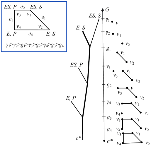
Fig. 8: The thermodynamic tree for the four–component enzyme–substrate system $S$, $E$, $ES$ $P$ (Fig. 4) with excess of substrate: $b_{S}>b_{E}$ (case (a)). The vertices and edges are enumerated in order of $\gamma_{v}$ and $g_{e}$ (starting from the greatest values). The order of these numbers is represented in Fig. On the right, the graphs $\widetilde{D_{1}}\setminus U_{g}$ are depicted. The solid bold line on the tree is the thermodynamically admissible path from the initial state $E,S$ (enzyme plus substrate) to the equilibrium. There are leaves at all levels $g=\gamma_{i}$. There are branching points at $g=g_{1,2,3}$ and no vertices at $g=g_{4}$.

In this section, we present two example of the thermodynamic tree. First, let us consider the trapezium (Fig. 4a). Let us select the order of numbers $\gamma_{v}$ and $g_{e}$ according to Fig. 8. The vertices and edges are enumerated in order of $\gamma_{v}$ and $g_{e}$ (starting from the greatest values). The tree is presented in Fig. 8. On the right, the graphs $\widetilde{D_{1}}\setminus U_{g}$ are depicted for all intervals $(a_{i-1},a_{i}]$. For $(\gamma_{2},\gamma_{1}]$ it is just a vertex $v_{1}$. For $(g_{1},\gamma_{2}]$ it consists of two disjoint vertices, $v_{1}$ and $v_{2}$. For $(\gamma_{3},g_{1}]$ these two vertices are connected by an edge. On the interval $(g_{2},\gamma_{3}]$ the graph $\widetilde{D_{1}}\setminus U_{g}$ is an edge $(v_{1},v_{2})$ and an isolated vertex $v_{3}$. On $(\gamma_{4},g_{2}]$ all three vertices $v_{1}$, $v_{2}$ and $v_{3}$ are connected by edges. For $(g_{3},\gamma_{4}]$ the isolated vertex $v_{4}$ is added to the graph $\widetilde{D_{1}}\setminus U_{g}$. For $g\leq g_{3}$ the graph $\widetilde{D_{1}}\setminus U_{g}$ includes all the vertices and is connected.

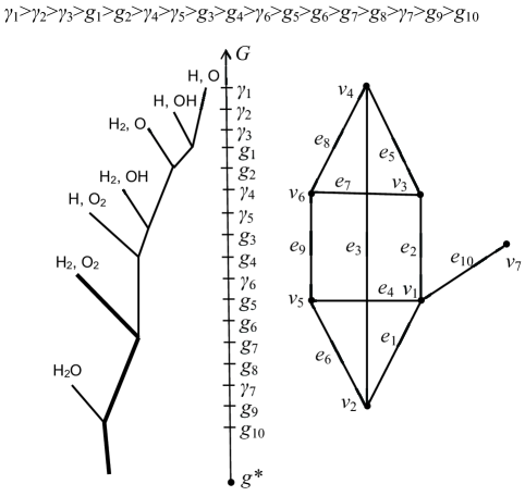
Fig. 9: The thermodynamic tree for the six–component ${\rm H}_{2}$–${\rm O}_{2}$ system, ${\rm H}_{2}$, ${\rm O}_{2}$, ${\rm H}$, ${\rm O}$, ${\rm H}_{2}{\rm O}$, ${\rm OH}$ with the stoichiometric hydrogen–oxygen ratio, $b_{\rm H}=2b_{\rm O}$ (Fig. 5b). The order of numbers $\gamma_{i}$, $g_{j}$ is presented in Fig. On the right, the graph $\widetilde{D_{1}}\setminus U_{g}$ is represented for $g=g_{10}$. For $g\leq g_{10}$, the graph $\widetilde{D_{1}}\setminus U_{g}$ includes all the vertices and is connected. The solid bold line on the tree is the thermodynamically admissible path from the initial state ${\rm H}_{2},{\rm O}_{2}$ to the equilibrium. There are leaves at all levels $g=\gamma_{i}$. There are branching points at $g=g_{1-4,7,10}$ and no vertices at $g=g_{5,6,8,9}$.

For the second example (Fig. 9) we selected the six-component system (Fig. 5) with the stoichiometric hydrogen–oxygen ratio, $b_{\rm H}=2b_{\rm O}$. The selected order of numbers $\gamma_{i}$, $g_{j}$ is presented in Fig. 9.

5 Conclusion

We studied dynamical systems that obey a continuous strictly convex Lyapunov function $G$ in a positively invariant convex polyhedron $D$. Convexity allows us to transform $n$-dimensional problems about attainability and attainable sets into an analysis of 1D continua and discrete objects.

We construct the tree (the Adelson-Velskii – Kronrod – Reeb tree [1, 42, 56]) of the function $G$ in $D$ and call this 1D continuum the thermodynamic tree.

The thermodynamic tree is a tool to solve the “attainability problem”: is there a continuous path between two states, $x$ and $y$ along which the conservation laws hold, the concentrations remain non-negative and the relevant thermodynamic potential $G$ (Gibbs energy, for example) monotonically decreases? This question arises often in non-equilibrium thermodynamics and kinetics. The analysis of the admissible paths can be considered as a dynamical analogue of the study of the steady states feasibility in chemical and biochemical kinetics. In this recent study, the energy balance method, the stoichiometric network theory, the entropy production analysis and the advanced algorithms of convex geometry of polyhedral cones are used [8, 54].

The obvious inequality, $G(x)\geq G(y)$ is necessary but not sufficient condition for existence of an admissible path from $x$ to $y$. In 1D systems, the space of states is an interval and the thermodynamic tree has two leaves (the ends of the interval) and one root (the equilibrium). In such a system, a spontaneous transition from a state $x$ to a state $y$ is allowed by thermodynamics if $G(x)\geq G(y)$ and $x$ and $y$ are on the same side of the equilibrium, i.e. they belong to the same branch of the thermodynamic tree. This is just a well known rule: “it is impossible to overstep the equilibrium in one-dimensional systems”.

The construction of the thermodynamic tree gives us the multidimensional analogue of this rule. Let $\pi:D\to\mathcal{T}$ be the natural projection of the balance polyhedron $D$ on the thermodynamic tree $\mathcal{T}$. A spontaneous transition from a state $x$ to a state $y$ is allowed by thermodynamics if and only if $\pi(y)\in[\pi(x),\pi(N^{*})]$, where $N^{*}$ is the equilibrium and $[\pi(x),\pi(N^{*})]$ is the ordered segment.

In this paper, we developed methods for solving the following problems:

1. How to construct the thermodynamic tree $\mathcal{T}$?

2. How to solve the attainability problem?

3. How to describe the set of all states attainable from a given initial state $x$?

For this purpose, we analyzed the cutting of a convex polyhedron by a convex set and developed the algorithm for construction of the tree of level set components of a convex function in a convex polyhedron. In this algorithm, the restriction of $G$ onto the 1-skeleton of $D$ is used. This finite family of convex functions of one variable includes all necessary information for analysis of the tree of the level set component of the convex function $G$ of many variables.

In high dimensions, some steps of our analysis become computationally expensive. The most expensive operations are the convex hull (description of the convex hull of a finite set by linear inequalities) and the double description operations (description of the faces of a polyhedron given by a set of linear inequalities). Therefore, in high dimensions some of the problem may be modified, for example, instead of the explicit description of the convex hull it is possible to use the algorithm for solution of a problem: does a point belong to this convex hull [55]. The computational aspects of the discussed problems in higher dimensions deserve more attention and the proper modifications of the problems should be elaborated. For example, two following problems need to be solved efficiently:

• To find the maximal and the minimal value of any linear function $f$ in a class of thermodynamic equivalence;

• To evaluate the maximum and the minimum of ${\mathrm{d}}G/{\mathrm{d}}t$ in any class of thermodynamic equivalence: $-\overline{\sigma}\leq{\mathrm{d}}G/{\mathrm{d}}t\leq-\underline{\sigma}\leq 0.$

For any $w\in\mathcal{T}$, the solution of the first problem allows us to find an interval of values of any linear function of state in the corresponding class of thermodynamic equivalence. We can use the results of Sec. 2.2 to reformulate this problem as the convex programming problem.

The second problem gives us the possibility to consider dynamics of relaxation on $\mathcal{T}$. On each interval on $\mathcal{T}$ we can write

$$-\overline{\sigma}(g)\leq{\mathrm{d}}g/{\mathrm{d}}t\leq-\underline{\sigma}(g)\leq 0\,,$$ (17)

where the functions $\overline{\sigma}(g),\underline{\sigma}(g)\geq 0$ depend on the interval on $\mathcal{T}$.

This differential inequality (17) will be a tool for the study of the dynamics of relaxation and may be considered as a reduced kinetic model that substitutes dynamics on the $d$-dimensional balance polyhedron $D$ by dynamics on the one-dimensional dendrite. The problem of the construction of the reduced model (17) is closely related to the following problem [66]: “Can one establish a lower bound on the entropy production, in terms of how much the distribution function departs from thermodynamical equilibrium?” In 1982, C. Cercignani [12] proposed a simple linear estimate for $\underline{\sigma}(g)$ for the Boltzmann equation (Cercignani’s conjecture). After that, these estimates were studied and improved by many authors [15, 11, 65, 66] and now the state of art achieved for the Boltzmann equation gives us some hints how to create the relaxation model (17) on the thermodynamic tree for the general kinetic systems. This may be the next step in the study of the thermodynamic trees.

References

- [1] G. M. Adelson-Velskii, A. S. Kronrod, About level sets of continuous functions with partial derivatives, Dokl. Akad. Nauk SSSR, 49 (4) (1945), pp. 239–241
- [2] P. M. Alberti, B. Crell, A. Uhlmann, C. Zylka, Order structure (majorization) and irreversible processes, in Vernetzte Wissenschaften–Crosslinks in Natural and Social Sciences, P. J. Plath, E.-Chr. Hass, eds.; Logos Verlag, Berlin, Germany, 2008, pp. 281–290.
- [3] P. M. Alberti, A. Uhlmann, Stochasticity and Partial Order – Doubly Stochastic Maps and Unitary Mixing; Mathematics and its Applications 9, D. Reidel Publ. Company, Dordrecht-Boston-London, 1982.
- [4] V. I. Arnold, On the representability of functions of two variables in the form , Uspehy Math. Nauk, 12 (2) (1957), pp. 119–121.
- [5] V. I. Arnold, From Hilbert’s superposition problem to dynamical system, Fields Inst. Comm., 24 (1999), pp. 1–19.
- [6] M. L. Balinski, An Algorithm for Finding all Vertices of Convex Polyhedral Sets, SIAM J., 9 (1961), 72–88.
- [7] A. D. Bazykin, Nonlinear dynamics of interacting populations, World Scientific Publishing: Singapore, 1998.
- [8] D. A. Beard, H. Qian, J. B. Bassingthwaighte, Stoichiometric foundation of large-scale biochemical system analysis, in Modelling in Molecular Biology, G. Ciobanu and G. Rozenberg, eds.; Springer, Berlin-Heidelberg-New York 1 (2004), pp. 1–21.
- [9] V. I. Bykov, Comments on “Structure of complex catalytic reactions: thermodynamic constraints in kinetic modeling and catalyst evaluation”, Ind. Eng. Chem. Res., 26 (1987), pp. 1943–1944.
- [10] L. Boltzmann, Lectures on gas theory, U. of California Press, Berkeley, CA, 1964.
- [11] E. Carlen, M. Carvalho, Entropy production estimates for Boltzmann equations with physically realistic collision kernels, J. Statist. Phys., 74 (3-4) (1994), pp. 743–782.
- [12] C. Cercignani, H-theorem and trend to equilibrium in the kinetic theory of gases, Archiwum Mechaniki Stosowanej, 34 (3) (1982), pp. 231–241.
- [13] J.J. Charatonik, Unicoherence and Multicoherence, article f-8 in Encyclopedia of General Topology, Elsevier, 2003, pp. 331–333.
- [14] N. V. Chernikova, An algorithm for finding a general formula for nonnegative solutions of system of linear inequalities, USSR Computational Mathematics and Mathematical Physics, 5 (1965), pp. 228–233.
- [15] L. Desvillettes, Entropy dissipation rate and convergence in kinetic equations. Comm. Math. Phys., 123 (4) (1989), pp. 687–702.
- [16] H. Doraiswamy, V. Natarajan, Efficient algorithms for computing Reeb graphs, Computational Geometry, 42 (6-7) (2009), pp. 606–616.
- [17] A. Einstein, Strahlungs-Emission und -Absorption nach der Quantentheorie, Verhandlungen der Deutschen Physikalischen Gesellschaft, 18 (13/14) (1916). Braunschweig: Vieweg, pp. 318–323.
- [18] M. Feinberg, D. Hildebrandt, Optimal reactor design from a geometric viewpoint–I. Universal properties of the attainable region, Chem. Eng. Sci., 52 (1997), pp. 1637–1665.
- [19] C. Filippi-Bossy, J. Bordet, J. Villermaux, S. Marchal-Brassely, C. Georgakis, Batch reactor optimization by use of tendency models, Comput. Chem. Eng., 13 (1989), pp. 35–47
- [20] A. T. Fomenko, T. L. Kunii, eds., Topological Modeling for Visualization, Springer, Berlin, 1997.
- [21] K. Fukuda, A. Prodon, 1996. Double description method revisited, in Lecture Notes in Computer Science, vol. 1120. Springer-Verlag, Berlin, 1996, pp. 91–111.
- [22] J. Gagneur, S. Klamt, Computation of elementary modes: a unifying framework and the new binary approach, BMC Bioinformatics 2004, 5:175.
- [23] D. Glasser, D. Hildebrandt, C. Crowe, A geometric approach to steady flow reactors: the attainable region and optimisation in concentration space, Am. Chem. Soc., 1987, pp. 1803–1810.
- [24] A. N. Gorban, Invariant sets for kinetic equations, React. Kinet. Catal. Lett., 10 (1979), pp. 187–190.
- [25] A. N. Gorban, Methods for qualitative analysis of chemical kinetics equations, in Numerical Methods of Continuum Mechanics; Institute of Theoretical and Applied Mechanics: Novosibirsk, USSR, 1979; Volume 10, pp. 42–59.
- [26] A. N. Gorban, Equilibrium Encircling. Equations of Chemical Kinetics and their Thermodynamic Analysis, Nauka Publ., Novosibirsk, 1984.
- [27] A. N. Gorban, P. A. Gorban, G. Judge, Entropy: The Markov Ordering Approach, Entropy, 12 (5) (2010), pp. 1145–1193.
- [28] A. N. Gorban, B. M. Kaganovich, S. P. Filippov, A. V. Keiko, V. A. Shamansky, I. A. Shirkalin, Thermodynamic Equilibria and Extrema: Analysis of Attainability Regions and Partial Equilibria, Springer, New York, NY, 2006.
- [29] A. N. Gorban, G. S. Yablonskii, On one unused possibility in planning of kinetic experiment, Dokl. Akad. Nauk SSSR, 250 (1980), pp. 1171–1174.
- [30] A. N. Gorban, G. S. Yablonskii, Extended detailed balance for systems with irreversible reactions, Chem. Eng. Sci., 66 (2011), pp. 5388–5399.
- [31] A. N. Gorban, G. S. Yablonskii, V. I. Bykov, Path to equilibrium. In Mathematical Problems of Chemical Thermodynamics, Nauka, Novosibirsk, 1980, pp. 37–47 (in Russian). English translation: Int. Chem. Eng., 22 (1982), pp. 368–375.
- [32] P. M. Gruber, J. M. Wills (eds.), Handbook of Convex Geometry, Volume A, North-Holland, Amsterdam, 1993.
- [33] K. M. Hangos, Engineering model reduction and entropy-based Lyapunov functions in chemical reaction kinetics, Entropy, 12(4) (2010), pp. 772–797.
- [34] D. Hildebrandt, D. Glasser, The attainable region and optimal reactor structures, Chem. Eng. Sci., 45 (1990), pp. 2161–2168.
- [35] M. Hill, Chemical product engineering – the third paradigm, Comput. Chem. Eng., 33 (2009), pp. 947–953.
- [36] F. Horn, Attainable regions in chemical reaction technique, in The Third European Symposium on Chemical Reaction Engineering, Pergamon Press, London, UK, 1964, pp. 1–10.
- [37] B.M. Kaganovich, A.V. Keiko, V.A. Shamansky, Equilibrium Thermodynamic Modeling of Dissipative Macroscopic Systems, Advances in Chemical Engineering, 39, 2010, pp. 1–74.
- [38] S. Kauchali, W. C. Rooney, L. T. Biegler, D. Glasser, D. Hildebrandt, Linear programming formulations for attainable region analysis, Chem. Eng. Sci., 57 (2002), pp. 2015–2028.
- [39] J. Klemelä, Smoothing of multivariate data: density estimation and visualization, J. Wiley & Sons, Inc., Hoboken, NJ, 2009.
- [40] A. N. Kolmogorov, Sulla teoria di Volterra della lotta per l’esistenza, Giornale Instituto Ital. Attuari, 7 (1936), pp. 74–80.
- [41] F. J. Krambeck, Accessible composition domains for monomolecular systems, Chem. Eng. Sci., 39 (1984), pp. 1181–1184.
- [42] A. S. Kronrod, On functions of two variables, Uspechi Matem. Nauk, 5(1) (1950), pp. 24-134.
- [43] V. I. Manousiouthakis, A. M. Justanieah, L. A. Taylor, The Shrink-Wrap algorithm for the construction of the attainable region: an application of the IDEAS framework, Comput. Chem. Eng., 28 (2004), pp. 1563–1575.
- [44] V. P. Maslov, G. A Omel’yanov, Geometric Asymptotics for Nonlinear PDE. I (Translations of Mathematical Monographs), American Mathematical Society, Providence, 2001.
- [45] R. M. May, W. J. Leonard, Nonlinear Aspects of Competition Between Three Species, SIAM Journal on Applied Mathematics, 29 (1975), pp. 243–253.
- [46] C. McGregor, D. Glasser, D. Hildebrandt, The attainable region and Pontryagin’s maximum principle, Ind. Eng. Chem. Res., 38 (1999), pp. 652–659.
- [47] M. J. Metzger, D. Glasser, B. Hausberger, D. Hildebrandt, B. J. Glasser B.J. Use of the attainable region analysis to optimize particle breakage in a ball mill, Chem. Eng. Sci., 64, (2009), pp. 3766–3777.
- [48] J. Milnor, Morse Theory, Princeton University Press, Princeton, NJ, 1963.
- [49] T. S. Motzkin, H. Raiffa, G. L. Thompson, R. M. Thrall, The double description method, in Contributions of the Theory of Games II, H. W. Kuhn and A. W. Tucker, eds., Annals of Mathematics, 8 (1953), Princeton University Press, Princeton, N.J., pp. 51–73.
- [50] H. Nagamochi, T. Ibaraki, Algorithmic Aspects of Graph Connectivity, Cambridge University Press, New York, 2008.
- [51] L. Onsager, Reciprocal relations in irreversible processes. I, Phys. Rev., 37 (1931), pp. 405–426.
- [52] J. Pearl, R. E. Korf, Search Techniques, Ann. Rev. Comp. Sci., 2 (1987), 451–467.
- [53] R. Peierls, Model-Making in Physics, Contemp. Phys., 21 (1980), pp. 3–17.
- [54] H. Qian, D. A. Beard, Thermodynamics of stoichiometric biochemical networks in living systems far from equilibrium, Biophys. Chem., 114, (2-3), (2005), pp. 213–220.
- [55] F. P. Preparata, M. I. Shamos, Computational Geometry: An Introduction, Springer, New York, 1985
- [56] G. Reeb, Sur les points singuliers d une forme de Pfaff completement integrable ou d une fonction numerique, Comptes Rendus Acad. Sci. Paris 222 (1946), pp. 847–849.
- [57] R.T. Rockafellar, Convex Analysis, Princeton University Press: Princeton, NJ, USA, 1970. Reprint: 1997.
- [58] S. Schuster, D. A. Fell, T. Dandekar, A general definition of metabolic pathways useful for systematic organization and analysis of complex metabolic networks, Nat. Biotechnology, 18 March (2000), pp. 326–332.
- [59] A. I. Shafarevich, Asymptotic solutions of the Navier-Stokes equations and topological invariants of vector fields. Prandtl–Maslov equations on the Reeb graphs and Fomenko invariants, Russian J. Math. Phys., 7(2) (2000), pp. 401–447.
- [60] R. Shinnar, Thermodynamic analysis in chemical process and reactor design, Chem. Eng. Sci., 43 (1988), pp. 2303–2318.
- [61] R. Shinnar, C. A. Feng, Structure of complex catalytic reactions: thermodynamic constraints in kinetic modeling and catalyst evaluation, Ind. Eng. Chem. Fundam., 24 (1985), pp. 153–170.
- [62] K. Sigmung, Kolmogorov and population dynamics, in Kolmogorov s Heritage in Mathematics, É. Charpentier; A. Lesne, N. K. Nikolski, eds., Springer: Berlin, Germany, 2007; pp. 177–186.
- [63] R. L. Smith, M. F. Malone, Attainable regions for polymerization reaction systems, Ind. Eng. Chem. Res., 36 (1997), pp. 1076–1084.
- [64] W. Stuetzle, Estimating the cluster tree of a density by analyzing the minimal spanning tree of a sample, J. Classification 20(5) (2003), pp. 25–47.
- [65] G. Toscani, C. Villani, Sharp entropy dissipation bounds and explicit rate of trend to equilibrium for the spatially homogeneous Boltzmann equation, Comm. Math. Phys., 203 (3) (1999), pp. 667–706.
- [66] C. Villani, Cercignani’s conjecture is sometimes true and always almost true, Comm. Math. Phys., 234 (3) (2003), pp. 455–490.
- [67] R. Wegscheider, Über simultane Gleichgewichte und die Beziehungen zwischen Thermodynamik und Reactionskinetik homogener Systeme, Monatshefte für Chemie / Chemical Monthly, 32(8) (1911), pp. 849–906.
- [68] G. S. Yablonskii, V. I. Bykov, A. N. Gorban, V. I. Elokhin, Kinetic models of catalytic reactions, Comprehensive Chemical Kinetics, Vol. 32, R. G. Compton, ed., Elsevier, Amsterdam, 1991.
- [69] M. Zarodnyuk, A. Keiko, B. Kaganovich, Elaboration of attainability region boundaries in the model of extreme intermediate states, Studia Informatica Universalis, 9 (2011), pp. 161–175.
- [70] Ch. Zylka, A note on the attainability of states by equalizing processes, Theor. Chim. Acta, 68 (1985), pp. 363–377.