Metal-insulator transition in 2D random fermion systems of chiral symmetry classes

Abstract

Field-theoretical approach to Anderson localization in 2D disordered fermionic systems of chiral symmetry classes (BDI, AIII, CII) is developed. Important representatives of these symmetry classes are random hopping models on bipartite lattices at the band center. As was found by Gade and Wegner two decades ago within the sigma-model formalism, quantum interference effects in these classes are absent to all orders of perturbation theory. We demonstrate that the quantum localization effects emerge when the theory is treated non-perturbatively. Specifically, they are controlled by topological vortex-like excitations of the sigma models. We derive renormalization-group equations including these non-perturbative contributions. Analyzing them, we find that the 2D disordered systems of chiral classes undergo a metal-insulator transition driven by topologically induced Anderson localization. We also show that the Wess-Zumino and $\mathbb{Z}_{2}$ theta terms on surfaces of 3D topological insulators (in classes AIII and CII, respectively) overpower the vortex-induced localization.

I Introduction

Disorder-induced metal-insulator transitions represent a fundamental concept of modern condensed matter physics. The principal mechanism of this phenomenon is Anderson localization Anderson58 due to quantum interference between different trajectories of electron propagation in a disordered medium. As was realized in seventies by Thouless and Wegner Thouless74 ; Wegner76 , the problem of Anderson localization is closely connected to the scaling theory of critical phenomena. Several years later, Abrahams and coauthors formulated the scaling theory of localization AALR describing the problem in terms of a flow of the dimensionless conductance $g$ with the system size $L$. This phenomenological theory was put on a solid basis by Wegner Wegner79 who discovered the field-theoretical description of Anderson localization in terms of a nonlinear sigma model. The latter is an effective field theory of the problem, capturing all essential properties of the system including its symmetry and topology. The crucial importance of the topological aspect was first demonstrated by Pruisken in the framework of the quantum Hall effect Pruisken84 . The field-theoretical (sigma model) formulation of the problem underpins the notion of universality of critical behavior at metal-insulator transitions, i.e., its independence of microscopic details of the electron motion. Over the years the sigma model permitted the great progress in understanding localization phenomena including, in particular, critical behavior,Wegner79 ; Efetov97 ; Evers08 energy level and wave function statistics,Efetov97 ; Mirlin00 symmetry classification,Zirnbauer96 interaction (most prominently 2D metal-insulator transition) and non-equilibrium effects,Finkelstein90 ; BelitzKirkpatrick ; KamenevAndreev ; Punnoose theory of unconventional disordered superconductors,ASZ classification of topological insulators and superconductors.SchnyderKitaev

Recent years have witnessed increasing interest and significant progress in the field of the Anderson localization. Development of the complete symmetry classification of disordered systems Zirnbauer96 is one of most important advances. It has been realized that underlying symmetries and topologies induce a remarkable variety of the types of infrared (long-distance, low-temperature) behavior, including, in particular, critical phases and quantum phase transitions between metallic and insulating states Evers08 . Experimental discoveries of graphene graphene and of topological insulators Molenkamp ; HasanKane10 ; QiZhang11 have given an additional boost to the field. Disordered Dirac fermions in graphene in the absence of valley mixing and surface states of disordered topological insulators and superconductors are characterized by sigma models with Wess-Zumino or theta terms, ensuring a topological protection from localization Evers08 ; SchnyderKitaev ; AL50 .

The full symmetry classification of disordered fermion systems Zirnbauer96 ; Evers08 includes three families of symmetry classes: conventional (Wigner-Dyson), chiral, and superconducting (Bogoliubov-de Gennes). In this paper we will consider localization properties of two-dimensional (2D) chiral models. Characteristic feature of these systems is the chiral symmetry of the underlying Hamiltonian $H=-CHC^{-1}$, where $C^{2}=1$. It is convenient to use the block structure such that $C$ is represented by the third Pauli matrix $\tau_{z}$; then the Hamiltonian acquires a block off-diagonal form,

$$H=\begin{pmatrix}0&h\\ h^{\dagger}&0\end{pmatrix}.$$ (1)

One-dimensional disordered systems with chiral symmetry were studied in Refs. chiral1D, . An effective field-theoretical description – non-linear sigma model – for chiral Hamiltonians with randomness was developed in Refs. chiralsigmamodel, ; GadeWegner, . Spectral properties of chiral random matrix ensembles were discussed in the context of mesoscopic transport and quantum chromodynamics in Refs. chiralRMT, ; Ivanov02, .

A standard realization of a chiral system is provided by a bipartite lattice model (i.e., containing two sublattices) with random hopping between the sublattices and no diagonal disorder. The Hamiltonian of such a model at the band center is manifestly block off-diagonal in the sublattice space. In analogy with Wigner-Dyson classes, there are three chiral classes: chiral unitary (AIII), chiral orthogonal (BDI), and chiral symplectic (CII) classes. The class AIII describes chiral systems with broken time-reversal symmetry, which may be due to magnetic flux (random or homogeneous) through the lattice plaquettes. The classes BDI and CII are characterized, in addition to the chiral symmetry, by time-reversal invariance, $H=KH^{T}K^{-1}$, where the unitary matrix $K$ satisfies $K^{2}=\pm 1$. For the chiral orthogonal class BDI one has $K^{2}=1$; in the standard representation $K=1$. For the chiral symplectic class CII, which corresponds to the case of broken spin rotation symmetry (usually due to spin-orbit interaction), $K^{2}=-1$; in the standard representation $K=i\sigma_{y}$, where $\sigma_{y}$ is the second Pauli matrix in the spin space. Thus, in the standard form, random Hamiltonians of the chiral classes have block off-diagonal structure and consist of complex, real, and real quaternion entries for the classes AIII, BDI, and CII, respectively.

Realizations of 2D chiral classes arise naturally when one models the disordered graphene at the Dirac point OGM . Specifically, the chiral symmetry occurs if the dominant disorder is of random-hopping character. An important example is the random magnetic flux, either genuine or effective (due to lattice corrugations), in which case the system belongs to the chiral unitary class AIII. Another possible realization is provided by graphene with vacancies. A vacancy can be modeled by cutting all lattice bonds adjacent to the vacated site, so that vacancies represent a special type of bond disorder. This model is in the chiral orthogonal symmetry class BDI. If an external magnetic field is applied to graphene with vacancies, the time-reversal symmetry is broken and the system falls into the class AIII. Taking into account the spin-orbit interaction (in the absence of magnetic field) brings the system into the chiral symplectic symmetry class CII.

Clearly, the above symmetry analysis is not specific for graphene (hexagonal lattice) but is equally applicable to a random-hopping model on any other bipartite lattice (e.g. the square lattice) at the band center. The analysis of Anderson localization in the chiral classes performed in the present work is equally applicable to all such models.

A remarkable property of the three chiral symmetry classes in 2D is the exact absence of weak localization corrections to all orders in the perturbation theory GadeWegner . At the same time, when the disorder is strong enough, the transition to insulating state is inevitable. Indeed, consider a tight-binding Hamiltonian on a 2D bipartite (e.g., square or honeycomb) lattice. Let us introduce disorder by randomly cutting the lattice bonds. (As discussed above, this model belongs to the chiral orthogonal class BDI.) Classically, this is the standard percolation model with bond disorder. When the concentration of removed bonds reaches the critical value ($1/2$ for square lattice and $1-2\sin(\pi/18)\approx 0.65$ for honeycomb lattice), the system becomes disconnected and undergoes the classical percolation transition to the insulating state. Obviously, the conductivity of such a system (defined in the limit of the infinite system size) is zero. It is well known that, in Wigner-Dyson symmetry classes, such a classical percolation transition is preceded by the Anderson metal-insulator transition. Specifically, due to quantum interference, the conductivity of a quantum system becomes zero at the point where classically it would still conduct (the remaining bonds are still percolating). Does this happen also for models of chiral classes? The exact absence of quantum-interference effects to all orders GadeWegner suggests that the answer is negative. However, numerical simulations in Refs. Motrunich02, ; Bocquet03, do show a quantum localization transition in chiral classes. These papers explored numerically models with continuous disorder which are always conducting classically, and yet found a metal-insulator transition. Thus, there appears to be a contradiction between the absence of localization in the sigma-model analysis of Ref. GadeWegner, and the numerical results. This contradiction is resolved in the present paper.

We will show below that, while the analysis of Ref. GadeWegner, is fully correct to all orders of perturbation theory, the quantum interference effects do emerge in the sigma-model field theory when one considers non-perturbative effects related to topologically non-trivial, vortex-like excitations. The field-theoretical analysis of the quantum localization in chiral classes requiring a systematic study of such non-perturbative effects constitutes the subject of the paper.

Non-perturbative effects caused by vortices were considered in the works of BerezinskiiBerezinskii71 and Kosterlitz and ThoulessKosterlitzThouless in the context of planar 2D ferromagnet (XY model) and 2D superfluid flow. These systems are characterized by a $\mathrm{U}(1)$ field (direction of magnetization and phase of the condensate wa)ve function, respectively) and exhibit the temperature-driven Berezinskii-Kosterlitz-Thouless (BKT) phase transition between quasi-ordered (ferromagnetic or superfluid) and disordered (paramagnetic or normal fluid) phases caused by vortex unbinding. Renormalization group (RG) analysis of this phase transition was first developed by KosterlitzKosterlitz74 . Alternative descriptions of the same systems are provided by the Coulomb gas (see Ref. Minnhagen, for a review) and sine-Gordon models. RG equations for the sine-Gordon model, equivalent to Kosterlitz RG, were derived in Ref. Wiegman, in the one-loop order and later in Ref. Amit, with the two-loop accuracy. We will show that, in analogy with the BKT physics, vortices drive the localization transition in chiral classes. However, the emerging theory is more complicated and the character of transition is essentially different, since the symmetry group of the localization problem is different from $\mathrm{U}(1)$.

The layout of the paper is as follows. In Sec. II, we present the general structure of the sigma model for chiral symmetry classes, outline the proof of the absence of perturbative weak localization corrections, and identify the mechanism of non-perturbative effects. The general background-field formalism for the renormalization of the sigma model is developed in Sec. III and then applied to the calculation of perturbative corrections in Sec. IV. In Sec. V, we construct the vortex excitations and explore their effect on the conductivity. For this purpose, we derive a set of RG equations on the conductivity $\sigma$, Gade-term coupling $c$ (controlling the behavior of the density of states), and the vortex fugacity $y$. Its analysis reveals a metal-insulator transition. Therefore, we show that the chiral classes do exhibit quantum interference effects – the weak localization and the Anderson transition – driven by topological excitations in the sigma model. In Sec. VI we develop an alternative approach to non-perturbative renormalization in class AIII. This approach is based on a mapping of the original sigma-model with vortices onto a dual theory which has a character of generalized sine-Gordon theory. Section VII is devoted to the interplay of this topological localization with further possible topological properties of 2D chiral-class systems: the Wess-Zumino term in class AIII and the $\mathbb{Z}_{2}$ theta term in class CII. These terms in the sigma models emerge when the 2D systems are realized on surfaces of 3D topological insulators of the corresponding symmetry classes. We show that the vortex-induced topological localization becomes inefficient in the presence of such terms. The latter thus ensure the topological protection of the system from localization. Our results are summarized in Sec. VIII. Some technical details are presented in two Appendices.

II Preliminaries

Very generally, localization properties of a disordered system are described by the non-linear sigma model field theory. We will use the fermionic replica version of the sigma model. (Alternatively, the same analysis can be performed within the supersymmetry approach; we choose the replica formalism here since in this case the presentation turns out to be physically more transparent.) The sigma-model target space is a compact symmetric space, see Ref. Evers08, for a review. For the three chiral classes, the field $Q(\mathbf{r})$ is a unitary matrix taking values in the symmetric spaces listed in Table 1. The size of the $Q$ matrix, $N$, is determined by the number of replicas; in the end one should take the replica limit $N\to 0$. In each of the classes CII and BDI, the $Q$ matrix obeys a certain linear constraint. These constraints can be represented as $Q=\bar{Q}$, where the “bar” operation is defined in the following way:

$$\bar{Q}=\begin{cases}Q^{T},&\text{CII},\\ CQ^{T}C,&\text{BDI}.\end{cases}$$ (2)

In the class BDI, $C$ is a skew-symmetric matrix such that $C^{2}=1$. In the standard parametrization of the model, the number of replicas $N$ is even and includes the spin degree of freedom while the matrix $C$ is the $\sigma_{y}$ Pauli matrix acting in the spin subspace.

Class	Manifold	$Q$ matrix	$D$	$s$
AIII	$\mathrm{U}(N)$	No restriction	$N^{2}$	1
CII	$\mathrm{U}(N)/\mathrm{O}(N)$	$Q=Q^{T}$	$N(N+1)/2$	2
BDI	$\mathrm{U}(N)/\mathrm{Sp}(N)$	$Q=CQ^{T}C$	$N(N-1)/2$	2

Table 1: List of chiral symmetry classes including corresponding compact sigma-model manifolds, symmetry constraints on the $Q$ matrix, and the dimensionalities $D$ of the target spaces. Parameter $s$ in the last column is introduced to normalize the conductivity in Eq. (3).

The distinguishing feature of the three manifolds of chiral-class sigma models is that the corresponding tangent spaces possess a unit generator commuting with all other (traceless) generators. This generator corresponds to the $\mathrm{U}(1)$ part of the corresponding symmetric space. The presence of this special generator allows an additional Gade term in the sigma model action GadeWegner :

$$S[Q]=-\int\frac{d^{2}r}{8\pi s}\left[\sigma\mathop{\mathrm{Tr}}(Q^{-1}\nabla Q)^{2}+c(\mathop{\mathrm{Tr}}Q^{-1}\nabla Q)^{2}\right].$$ (3)

The parameter $\sigma$ is the dimensionless conductivity of the sample (measured in units $e^{2}/\pi h$)and $c$ multiplies the Gade term. The bare value of $c$ is of order $1$.

Let us decompose $Q$ according to $Q=e^{i\phi}U$ with $\det U=1$. The overall phase $\phi$ is exactly the $\mathrm{U}(1)$ degree of freedom characteristic for sigma models of the chiral symmetry classes. The action (3) takes the form

$$S[Q]=\int\frac{d^{2}r}{8\pi s}\left[N(\sigma+Nc)(\nabla\phi)^{2}+\sigma\mathop{\mathrm{Tr}}(\nabla U^{-1}\nabla U)\right].$$ (4)

We see that variables $\phi$ and $U$ decouple and that the action is quadratic in $\phi$. This means that the prefactor $\sigma+Nc$ of the $(\nabla\phi)^{2}$ term is not renormalized. In the replica limit $N\to 0$, the absence of localization corrections to $\sigma$ follows, which is the result of Gade and WegnerGadeWegner .

The above argument for the absence of the renormalization of conductivity has, however, a caveat. Specifically, the action for the variable $\phi$ is not strictly Gaussian in view of the compact $\mathrm{U}(1)$ nature of this degree of freedom. The group $\mathrm{U}(1)$ is not simply connected allowing for topological excitations – vortices. Fluctuations of the matrix $Q$ involving vortices yield corrections to $\sigma+Nc$ via the BKTBerezinskii71 ; KosterlitzThouless mechanism. These corrections break the replica symmetry and thus invalidate the Gade and Wegner argument. Our goal is to analyze the effect of vortices on the renormalization of the chiral-class sigma models. We will start with the general background field formulation of the renormalization. Then we will consider both perturbative and non-perturbing (due to vortices) contributions to the RG equations.

III Background field formalism

Very generally, renormalization of the sigma model can be implemented in the framework of the background field formalism Polyakov75 ; Pruisken87 . Following this approach, we first separate slow and fast parts in the matrix $Q$. The former is referred to as the background field. Then the partition function is integrated over the fast part of $Q$ yielding the effective action for the background field. This effective action has the same sigma-model form with the renormalized parameters $\sigma$ and $c$.

In order to renormalize the action (3), we parametrize $Q=\bar{V}\tilde{Q}V$, where $\tilde{Q}$ is the fast field of the same symmetry as $Q$ and unitary matrices $V$ and $\bar{V}$ represent the slow background field. In the symmetry class AIII, matrices $V$ and $\bar{V}$ are independent while for the other two chiral classes they are related by Eq. (2). After integrating out $\tilde{Q}$, the effective action involves only the gauge invariant combination of slow fields $Q^{\prime}=\bar{V}V$. It is convenient to introduce the following notations for the gradients of the slow field:

$$\mathbf{A}=\nabla VV^{-1},\qquad\bar{\mathbf{A}}=\bar{V}^{-1}\nabla\bar{V}.$$ (5)

Matrices $\mathbf{A}$ and $\bar{\mathbf{A}}$ are related by Eq. (2) in classes CII and BDI.

We start the renormalization group analysis with the action $S_{0}[Q]$ given by Eq. (3) with bare parameters $\sigma_{0}$ and $c_{0}$. Upon substitution $Q=\bar{V}\tilde{Q}V$, the action decomposes into four terms:

$$S_{0}[Q]=S_{0}[Q^{\prime}]+S_{L}[\tilde{Q}]+S_{\mathrm{int}}^{(1)}[\bar{V},V,\tilde{Q}]+S_{\mathrm{int}}^{(2)}[\bar{V},V,\tilde{Q}].$$ (6)

The first term, $S_{0}[Q^{\prime}]$, is the bare action for the slow background field $Q^{\prime}=\bar{V}V$. It can be represented as

$$S_{0}[Q^{\prime}]=-\!\!\int\!\frac{d^{2}r}{8\pi s}\left\{\!\sigma_{0}\mathop{\mathrm{Tr}}\left(\bar{\mathbf{A}}+\mathbf{A}\right)^{2}+c_{0}\left[\mathop{\mathrm{Tr}}\left(\bar{\mathbf{A}}+\mathbf{A}\right)\right]^{2}\right\}.$$ (7)

The action for the fast field $S_{L}[\tilde{Q}]$ is given by the same Eq. (3) with bare parameters $\sigma_{0}$ and $c_{0}$ but includes also the mass term,

$$S_{L}[\tilde{Q}]=S_{0}[\tilde{Q}]-\frac{\sigma_{0}}{8\pi sL^{2}}\int d^{2}r\mathop{\mathrm{Tr}}\big{(}2-\tilde{Q}-\tilde{Q}^{-1}\big{)}.$$ (8)

The mass $\sim 1/L$ is introduced to ensure that the matrix $\tilde{Q}$ contains only fast degrees of freedom. At the same time, we will assume that the slow fields $V$ and $\bar{V}$ change very little on the distances of the order of $L$. It is important that the mass term is symmetric on the manifold of $\tilde{Q}$; this will guarantee that the renormalized action involves only the gauge-invariant combination $\bar{V}V$ and retains the full symmetry of the sigma model. Finally, the terms in the action representing the interaction between the slow and fast modes read

$$S_{\mathrm{int}}^{(1)} =-\int\frac{d^{2}r}{4\pi s}\Big{[}\sigma_{0}\mathop{\mathrm{Tr}}\left(\nabla\tilde{Q}\tilde{Q}^{-1}\bar{\mathbf{A}}+\tilde{Q}^{-1}\nabla\tilde{Q}\mathbf{A}\right)$$

$$\hskip 42.67912pt+c_{0}\mathop{\mathrm{Tr}}\tilde{Q}^{-1}\nabla\tilde{Q}\mathop{\mathrm{Tr}}\left(\bar{\mathbf{A}}+\mathbf{A}\right)\Big{]},$$ (9)

$$S_{\mathrm{int}}^{(2)} =\sigma_{0}\int\frac{d^{2}r}{4\pi s}\mathop{\mathrm{Tr}}\left[\bar{\mathbf{A}}\mathbf{A}-\tilde{Q}^{-1}\bar{\mathbf{A}}\tilde{Q}\mathbf{A}\right].$$ (10)

Integrating $e^{-S[Q]}$ over fast modes $\tilde{Q}$, taking the logarithm of the result, performing the gradient expansion, and retaining the terms with two spatial derivatives (i.e. up to second order in $\mathbf{A}$ and $\bar{\mathbf{A}}$), we obtain the effective action for the slow field:

$$S[Q^{\prime}]=S_{0}[Q^{\prime}]+\left<S_{\mathrm{int}}^{(2)}\right>-\frac{1}{2}\left<\big{[}S_{\mathrm{int}}^{(1)}\big{]}^{2}\right>.$$ (11)

Here $\langle\dots\rangle$ denotes the averaging over $\tilde{Q}$ with the weight $e^{-S_{L}[\tilde{Q}]}$. Note that the average $\langle S_{\mathrm{int}}^{(1)}\rangle$ is linear in the gradients of the slow variables and is hence zero. The renormalizability of the sigma model implies that the effective action for the slow field $Q^{\prime}$ has the form of Eq. (7) with the bare parameters $\sigma_{0}$ and $c_{0}$ replaced with their renormalized values $\sigma$ and $c$. Using this fact, we will assume three particular forms of the background field and thus establish the renormalized parameters in terms of $\tilde{Q}$ integrals for all three symmetry classes.

The $D$-dimensional sigma-model target space is generated by $D-1$ traceless Hermitian generators and one generator proportional to the unit matrix. In the classes CII and BDI these generators are subject to an additional symmetry constraint $T=\bar{T}$. We normalize the generators as $\mathop{\mathrm{Tr}}T^{a}T^{b}=\delta^{ab}$. The traceless generators of the sigma-model manifold obey the following Fierz identities:

$$\sum_{a}T^{a}_{ij}T^{a}_{kl}=\begin{cases}\delta_{il}\delta_{jk}-\dfrac{1}{N}\,\delta_{ij}\delta_{kl},&\text{AIII},\\[6.0pt] \dfrac{1}{2}\left(\delta_{il}\delta_{jk}+\delta_{ik}\delta_{jl}\right)-\dfrac{1}{N}\,\delta_{ij}\delta_{kl},&\text{CII},\\[6.0pt] \dfrac{1}{2}\left(\delta_{il}\delta_{jk}+C_{ik}C_{jl}\right)-\dfrac{1}{N}\,\delta_{ij}\delta_{kl},&\text{BDI}.\end{cases}$$ (12)

Assume the background field of the form $\mathbf{A}=\bar{\mathbf{A}}=i\mathbf{J}T$ with some constant vector $\mathbf{J}$ and $T$ being one of the $D-1$ traceless generators of the sigma-model manifold. Substituting this background field into Eq. (11), averaging over directions of $\mathbf{J}$, and comparing the prefactors of $\mathbf{J}^{2}$ in the left- and right-hand side of the equation, we find the renormalized conductivity in the form

$$\sigma=\sigma_{0}-\frac{\sigma_{0}}{4A}\int d^{2}r\mathop{\mathrm{Tr}}\left<\big{[}\tilde{Q},T\big{]}\big{[}\tilde{Q}^{-1},T\big{]}\right>\\ +\frac{\sigma_{0}^{2}}{32\pi sA}\left<\left[\int d^{2}r\mathop{\mathrm{Tr}}\big{\{}\nabla\tilde{Q},\tilde{Q}^{-1}\big{\}}T\right]^{2}\right>.$$ (13)

Next, we assume a pure gauge background field such that $\mathbf{A}=-\bar{\mathbf{A}}=i\mathbf{J}t$. The matrix $t$ is now one of generators of the stabilizer group, $\mathrm{U}(N)$, $\mathrm{O}(N)$, and $\mathrm{Sp}(N)$, for the classes AIII, CII, and BDI, respectively. These generators obey the second Fierz identity

$$\sum_{a}t^{a}_{ij}t^{a}_{kl}=\begin{cases}\delta_{il}\delta_{jk},&\text{AIII},\\[6.0pt] \dfrac{1}{2}\left(\delta_{il}\delta_{jk}-\delta_{ik}\delta_{jl}\right),&\text{CII},\\[6.0pt] \dfrac{1}{2}\left(\delta_{il}\delta_{jk}-C_{ik}C_{jl}\right),&\text{BDI}.\end{cases}$$ (14)

Such a gauge background field corresponds to the constant $Q^{\prime}=1$ and hence the left-hand side of Eq. (11) vanishes. Averaging over directions of $\mathbf{J}$, we obtain the following Ward identity

$$0=\frac{\sigma_{0}}{4A}\int d^{2}r\mathop{\mathrm{Tr}}\left<\big{[}\tilde{Q},t\big{]}\big{[}\tilde{Q}^{-1},t\big{]}\right>\\ +\frac{\sigma_{0}^{2}}{32\pi sA}\left<\left[\int d^{2}r\mathop{\mathrm{Tr}}\big{[}\nabla\tilde{Q},\tilde{Q}^{-1}\big{]}t\right]^{2}\right>.$$ (15)

We sum up identities (13) with all generators $T$ and add identities (15) with all possible matrices $t$. With the help of the Fierz identities (12) and (14) and using the properties $Q=\bar{Q}$ in the classes CII and BDI, we obtain the renormalized conductivity

$$\sigma=\sigma_{0}+\frac{\sigma_{0}^{2}}{D-1}\left(B_{1}-\frac{B_{2}}{N}\right).$$ (16)

Here we have introduced the averages

$$B_{1} =\int\frac{d(\mathbf{r-r^{\prime}})}{8\pi s}\left<\mathop{\mathrm{Tr}}\big{(}\tilde{Q}^{-1}\nabla\tilde{Q}\big{)}_{r}\big{(}\tilde{Q}^{-1}\nabla\tilde{Q}\big{)}_{r^{\prime}}\right>,$$ (17)

$$B_{2} =\int\frac{d(\mathbf{r-r^{\prime}})}{8\pi s}\left<\mathop{\mathrm{Tr}}\big{(}\tilde{Q}^{-1}\nabla\tilde{Q}\big{)}_{r}\mathop{\mathrm{Tr}}\big{(}\tilde{Q}^{-1}\nabla\tilde{Q}\big{)}_{r^{\prime}}\right>.$$ (18)

Finally, consider the background field of the form $\mathbf{A}=\bar{\mathbf{A}}=i\mathbf{J}\mathbbm{1}/\sqrt{N}$ generated by the unit matrix. This field configuration brings into play both the kinetic and the Gade terms of the action. After averaging over directions of $\mathbf{J}$, we obtain the identity

$$\sigma+Nc=\sigma_{0}+Nc_{0}+\frac{(\sigma_{0}+Nc_{0})^{2}}{N}\;B_{2}.$$ (19)

With $\sigma$ from Eq. (16), this yields the following expression for the renormalized coupling $c$:

$$c=c_{0}-\frac{\sigma_{0}^{2}\,B_{1}}{N(D-1)}+\left[\frac{\sigma_{0}^{2}}{D-1}+(\sigma_{0}+Nc_{0})^{2}\right]\frac{B_{2}}{N^{2}}.$$ (20)

Equations (16) and (20) represent renormalization of $\sigma$ and $c$ in the most general form. The averages $B_{1,2}$ implicitly depend on the infrared scale $L$ set by the mass term in the fast field action (8). The RG flow equations are obtained in the standard way by taking the derivative of Eqs. (16) and (20) with respect to $\ln L$ and replacing $\sigma_{0}$ and $c_{0}$ in the right-hand side of these equations with the running, $L$-dependent values $\sigma$ and $c$ of the couplings.

IV Perturbative renormalization

In the previous section we have developed the background field formalism and reduced the renormalization of the sigma models of chiral classes to the calculation of the correlators (17) and (18). The matrix $\tilde{Q}$ belongs to the corresponding sigma-model manifold and averaging is performed with the statistical weight determined by the action (8). We will now perform this averaging using a saddle point method. The saddle point approximation is justified in the limit $\sigma_{0}\gg 1$. We start with the spatially uniform saddle point $\tilde{Q}=1$. Note that the mass term in the action (8) is minimized by this, rather than any other, constant value of $\tilde{Q}$. Expansion in the vicinity of the spatially uniform saddle point yields perturbative contributions to the renormalized couplings. As we are going to explain, such perturbative correction to $\sigma$ vanishes, in the replica limit $N\to 0$, in all orders of the perturbation theory for all three chiral classes. We will then proceed by including a non-perturbative contribution from saddle configurations containing a vortex-antivortex dipole. We will show that this yields a non-zero result.

We parametrize the fast field $\tilde{Q}=1+iW-W^{2}/2+O(W^{3})$ by a Hermitian matrix $W$ subjected to the linear constraint $W=\bar{W}$ in classes CII and BDI. Let us decompose $W$ in generators of the corresponding symmetric space: $W=w_{0}\mathbbm{1}/\sqrt{N}+\sum_{a}w_{a}T^{a}$. Expanding Eq. (8) to the second order in $W$, we obtain the Gaussian action

$$S_{L}[W]=\int\frac{d^{2}r}{8\pi s}\bigg{\{}(\sigma_{0}+Nc_{0})(\nabla w_{0})^{2}+\sigma_{0}L^{-2}w_{0}^{2}\\ +\sigma_{0}\sum_{a}\Big{[}(\nabla w_{a})^{2}+L^{-2}w_{a}^{2}\Big{]}\bigg{\}}.$$ (21)

This action yields the following propagators of the components of $W$:

$$\langle w_{0}(\mathbf{q})w_{0}(-\mathbf{q})\rangle =\frac{4\pi s}{(\sigma_{0}+Nc_{0})q^{2}+\sigma_{0}L^{-2}},$$ (22)

$$\langle w_{a}(\mathbf{q})w_{a}(-\mathbf{q})\rangle =\frac{4\pi s}{\sigma_{0}(q^{2}+L^{-2})}.$$ (23)

Within the perturbative calculation, the average $B_{2}$ is identically zero since it involves only the $\mathrm{U}(1)$ component of $\tilde{Q}$; specifically, $\mathop{\mathrm{Tr}}\tilde{Q}^{-1}\nabla\tilde{Q}=i\sqrt{N}\nabla w_{0}$. Consequently, $B_{2}$ vanishes, $B_{2}\propto q^{2}\langle w_{0}(\mathbf{q})w_{0}(-\mathbf{q})\rangle_{q\to 0}=0$, that implies that $\sigma+Nc$ is not renormalized, see Eq. (19). This cancellation of $B_{2}$ is the essence of the Gade-Wegner argument GadeWegner for the absence of weak localization corrections to conductivity. We will see later that the saddle points involving vortices yield a nonvanishing contribution to $B_{2}$.

Contrary to $B_{2}$, the average $B_{1}$ is non-zero already on the perturbative level. We will calculate it within the one-loop approximation. Rewriting Eq. (17) in the momentum representation, expanding in the components of $W$, and applying the Wick theorem, we find

$$B_{1}=\int\frac{q^{2}\,d^{2}q}{32\pi^{3}s}\Big{[}\big{<}W_{ij}(\mathbf{q})W_{kl}(-\mathbf{q})\big{>}\big{<}W_{jk}(\mathbf{q})W_{li}(-\mathbf{q})\big{>}\\ -\big{<}W_{ij}(\mathbf{q})W_{jk}(-\mathbf{q})\big{>}\big{<}W_{kl}(\mathbf{q})W_{li}(-\mathbf{q})\big{>}\Big{]}.$$ (24)

We have dropped the term $\sim q^{2}\langle W^{2}\rangle|_{q\to 0}$. The absence of such a term is justified by the finite mass in the action (21) and hence a finite limit of the $W$ propagator at $q\to 0$. Using the decomposition of $W$ in generators $T$ and the propagators (22) and (23), we obtain $B_{1}$ in the form

$$B_{1}=\int^{\Lambda}\frac{s\;q^{3}\;dq}{2\sigma_{0}^{2}(q^{2}+L^{-2})^{2}}\sum_{a,b}\mathop{\mathrm{Tr}}\big{[}T^{a},T^{b}\big{]}^{2}.$$ (25)

Note that the propagator $\langle w_{0}w_{0}\rangle$ is canceled in the expression for $B_{1}$. The momentum integral is logarithmically divergent and we have introduced the ultraviolet cut-off $\Lambda$ to regularize this divergence.

Using the appropriate Fierz identity, we calculate the trace of products of four generators and obtain the result

$$B_{1}\simeq N(1-D)\frac{\ln(\Lambda L)}{\sigma_{0}^{2}}.$$ (26)

Substituting this result and $B_{2}=0$ into Eqs. (16) and (20), we obtain logarithmic corrections to $\sigma$ and $c$ that can be recast in the form of renormalization group equations

$$\frac{\partial\sigma}{\partial\ln L} =-N+NO(1/\sigma),$$ (27)

$$\frac{\partial c}{\partial\ln L} =1+O(1/\sigma).$$ (28)

These equations describe the real space scaling with the running infrared cut-off length $L$. The higher loop contributions provide $O(1/\sigma)$ terms in the perturbative RG equations. In the replica limit, renormalization of $\sigma$ vanishes, in full agreement with the argument by Gade and Wegner GadeWegner .

A remarkable feature of the perturbative renormalization in class AIII is that the right-hand side of Eq. (28) is exactly $1$ in the limit $N\to 0$. Higher loop contributions to the beta function for $c$ are proportional to $N$ and vanish in the replica limit.Guruswamy ; Elio This is not the case in the other two chiral symmetry classes. The exact perturbative RG equations in class AIII can be applied even when $\sigma$ is not large. We will use this fact below for constructing the non-perturbative RG flow diagram.

V Non-perturbative renormalization

In order to find a correction to conductivity that does not vanish in the limit $N\to 0$, we have to consider the saddle-point configurations other than $\tilde{Q}=1$. These configurations will include vortices. Vortices are singular points of the $Q$ matrix such that the overall phase $\phi$ of $Q$ rotates by $2\pi$ along any path going around the vortex.

The sigma-model description with small gradients of $Q$ breaks down at distances of the order of the mean free path from the vortex center. This region, referred to as the vortex core, should be excluded from the sigma model action (3). The contribution of the vortex core to the overall action, $S_{v}$, is not universal and depends on details of the ballistic electron dynamics inside the core. Generically, $S_{v}\propto\sigma_{0}$. This introduces a new coupling constant in our theory, referred to as fugacity, $y_{0}=e^{-S_{v}}$, that is the statistical weight associated with the vortex core.

V.1 Vortex configurations

Let us construct explicitly the vortex configuration in three chiral classes. The minimal model of classes AIII and CII with a single replica reduces to the abelian $\mathrm{U}(1)$ model with $\tilde{Q}=e^{i\phi}$. The same situation occurs in class BDI at the minimum number of replicas $N=2$. In the latter case the matrix $\tilde{Q}$ retains the $2\times 2$ spin structure: $\tilde{Q}=e^{i\phi}\mathbbm{1}$. In all three models, the action (8) has the form (we neglect the mass term for simplicity)

$$S[\tilde{Q}]=\frac{K}{2\pi}\int d^{2}r(\nabla\phi)^{2},$$ (29)

where we have introduced the stiffness parameter

$$K=\begin{cases}(\sigma+c)/4,&\text{AIII},\\ (\sigma+c)/8,&\text{CII},\\ (\sigma+2c)/4,&\text{BDI}.\end{cases}$$ (30)

Assume a set of vortices with positions $\mathbf{r}_{i}$ and charges (vorticities) $n_{i}=\pm 1$. Such a configuration creates the gradient of $\phi$ given by

$$\nabla_{a}\phi(\mathbf{r})=\epsilon_{ab}\sum_{i}n_{i}\nabla_{b}\ln|\mathbf{r}-\mathbf{r}_{i}|.$$ (31)

Indeed, this field $\phi$ satisfies the equation of motion $\nabla^{2}\phi=0$ with additional condition of $2\pi n_{i}$ winding of $\phi$ around every vortex. The mass term in the action (8), which we have temporarily neglected in Eq. (29), requires $\phi=0$ at infinity. This is only possible if the system of vortices is neutral: $\sum_{i}n_{i}=0$. Thus the simplest allowed configuration of vortices is a vortex-antivortex pair, i.e., a dipole. Configurations with more than two vortices or vortices with higher winding numbers have lower statistical weight and can be safely neglected.

Let us consider an individual dipole with vortex and antivortex at positions $\mathbf{r}_{1,2}$. The separation between these points, $\mathbf{m}=\mathbf{r}_{1}-\mathbf{r}_{2}$, will be called the dipole moment. Substituting Eq. (31) into Eq. (29), we find the action for the dipole:

$$S_{m}=2S_{v}+2K\ln(\Lambda|\mathbf{m}|).$$ (32)

Here $\Lambda$ is the ultraviolet cut-off of the order of inverse radius of the vortex core. The action $2S_{v}$ associated with two vortex cores is explicitly added. We see that the action of the dipole grows logarithmically with increasing $m$. This is true provided the dipole is smaller than the infrared length $L$. For larger dipoles, the mass term will modify the dipole saddle point, and the action will grow linearly with $m$. Thus we conclude that the infrared cut-off $L$ in the $\tilde{Q}$ theory effectively limits the maximum allowed size of a dipole.

Let us now consider a general situation with arbitrary number of replicas. In class AIII, we place the dipole in the first replica and represent the matrix $\tilde{Q}$ as

$$\tilde{Q}_{m}=\mathbbm{1}+|p\rangle(e^{i\phi}-1)\langle p|.$$ (33)

Here $|p\rangle=\{1,0,0,\dots\}$ is the $N$-component vector in the replica space. We can generate other dipole configurations with the same action (32) by moving and rotating the dipole in the real space, which changes just the function $\phi$, and also by rotations $\tilde{Q}_{m}\mapsto\bar{V}\tilde{Q}_{m}V$ in replica space with spatially constant unitary matrices $V$ and $\bar{V}$. The mass term in Eq. (8) requires $\tilde{Q}_{m}=\mathbbm{1}$ at infinity and thus restricts the matrices by $\bar{V}V=1$. Such unitary rotations lead to the same form of $\tilde{Q}_{m}$ given by Eq. (33) with an arbitrary $N$-dimensional complex unit vector $|p\rangle$. Thus equivalent dipole configurations in replica space span the manifold $\mathrm{CP}^{N-1}=\mathrm{U}(N)/\mathrm{U}(N-1)\times\mathrm{U}(1)=S^{2N-1}/S^{1}$.

In class CII, additional constraint $\bar{V}=V^{T}$ applies, see Eq. (2). As a result, allowed rotations generate an arbitrary unit real vector $|p\rangle$ with $N$ components. The corresponding space is $\mathrm{RP}^{N-1}=\mathrm{O}(N)/\mathrm{O}(N-1)\times\mathrm{O}(1)=S^{N-1}/S^{0}$. Finally, in class BDI, the constraint (2) leads to the unit vector $|p\rangle$ composed of $N/2$ real quaternions. The corresponding manifold is $\mathrm{HP}^{N/2-1}=\mathrm{Sp}(N)/\mathrm{Sp}(N-2)\times\mathrm{Sp}(2)=S^{2N-1}/S^{3}$. The spaces of equivalent dipole configurations are listed in Table 2 together with their volumes $V_{p}$. In all three chiral symmetry classes $V_{p}=O(1/N)$ in the replica limit $N\to 0$.

Class	Null-space	$V_{p}$
AIII	$\mathrm{CP}^{N-1}$	$\pi^{N-1}/\Gamma(N)$
CII	$\mathrm{RP}^{N-1}$	$\pi^{N/2-1}/\Gamma(N/2)$
BDI	$\mathrm{HP}^{N-1}$	$\pi^{N-2}/\Gamma(N)$

Table 2: List of spaces spanned by equivalent dipole configurations. Volumes of these spaces are denoted by $V_{p}$.

V.2 Derivation of RG equations

The contribution of the dipole to the correlation functions $B_{1,2}$ of the fast field $\tilde{Q}$ is found by substituting $\tilde{Q}=\tilde{Q}_{m}$ from Eq. (33) into Eqs. (17) and (18) and calculating the Gaussian integral of quadratic fluctuations around the dipole saddle point. The result has the form

$$B_{1,2}^{\text{dip}}=\Lambda^{4}\int d^{2}R\,d^{2}m\,\frac{Z^{\prime}_{\text{dip}}}{Z_{0}}\;V_{p}\,\tilde{B}_{1,2}^{\text{dip}}\,e^{-S_{m}}.$$ (34)

Here $S_{m}$ is the action (32) associated with the dipole, $Z^{\prime}_{\text{dip}}$ and $Z_{0}$ are the partition functions of quadratic fluctuations near the dipole configuration and near the trivial uniform minimum of the action, respectively. Zero modes related to rotations of the dipole in replica space are excluded from the determinant $Z^{\prime}_{\text{dip}}$; they yield the volume $V_{p}$ of the space of equivalent dipoles, see Table 2. Zero-modes related to the position $\mathbf{R}$ of the center of mass of the dipole and nearly-zero modes related to the dipole size $m$ are excluded from $Z^{\prime}_{\text{dip}}$ as well and are taken into account in Eq. (34) via integration over the corresponding collective coordinates. The factor $\Lambda^{4}$ arises when the partition sum over positions of vortex and antivortex, with the core size $\sim 1/\Lambda$, is replaced by the integral over $\mathbf{R}$ and $\mathbf{m}$. (Appearance of this factor is clear on dimensional reasons.) Finally, the pre-exponential factors $\tilde{B}_{1,2}^{\text{dip}}$ are given by expressions inside angular brackets in Eqs. (17) and (18) evaluated on $\tilde{Q}_{m}$ from Eq. (33).

The two vortices forming the dipole are located at $\mathbf{R}\pm\mathbf{m}/2$. From Eqs. (31) and (33), we obtain

$$\tilde{Q}_{m}^{-1}\nabla_{\mu}\tilde{Q}_{m}=-i\nabla_{\mu}\phi(\mathbf{r})\;|p\rangle\langle p|\\ =-i\epsilon_{\mu\nu}\nabla_{\nu}\ln\left|\frac{\mathbf{r}-\mathbf{R}-\mathbf{m}/2}{\mathbf{r}-\mathbf{R}+\mathbf{m}/2}\right|\;|p\rangle\langle p|.$$ (35)

In order to calculate $\tilde{B}_{1,2}^{\text{dip}}$, we substitute this expression into Eqs. (17) and (18). Afterwards, Eq. (34) is used to find $B_{1,2}^{\text{dip}}$. The projective property of the matrix (35) and the trace structure of Eqs. (17) and (18) imply the relation

$$B_{2}^{\text{dip}}=uB_{1}^{\text{dip}},$$ (36)

where we have introduce the notation $u=\mathop{\mathrm{Tr}}|p\rangle\langle p|$. In the classes AIII and CII, $u=1$, while in the class BDI we have $u=2$. The quantity $u$ can be interpreted as the minimal value of the number of replicas $N$ allowed by the symmetry.

In view of the identity (36), it suffices to calculate $B_{1}^{\text{dip}}$. When the dipole position is fixed, the integrand in Eq. (17) depends explicitly on both $\mathbf{r}$ and $\mathbf{r}^{\prime}$ rather than on their difference only. The uniformity is restored after integration over $\mathbf{R}$ in Eq. (34). Thus we will carry out the integration over the dipole positions first.

Equations (17), (34), and (35) combine into

$$B_{1}^{\text{dip}}=-\frac{u\,V_{p}}{8\pi s}\;\Lambda^{4}\int d^{2}p\,\frac{Z^{\prime}_{\text{dip}}(p)}{Z_{0}}\;e^{-S_{m}}\\ \times\!\!\int\!\!d(\mathbf{r-r^{\prime}})\,d^{2}R\,\nabla\ln\left|\frac{\mathbf{r}-\mathbf{R}-\frac{\mathbf{m}}{2}}{\mathbf{r}-\mathbf{R}+\frac{\mathbf{m}}{2}}\right|\nabla^{\prime}\ln\left|\frac{\mathbf{r}^{\prime}-\mathbf{R}-\frac{\mathbf{m}}{2}}{\mathbf{r}^{\prime}-\mathbf{R}+\frac{\mathbf{m}}{2}}\right|.$$ (37)

By construction, gradients in Eq. (37) act on $\mathbf{r}$ and $\mathbf{r}^{\prime}$. Equivalently, we can assume that both gradients act on $\mathbf{R}$. Integrating by parts and using the identity $\nabla^{2}\ln|\mathbf{R}|=2\pi\delta(\mathbf{R})$, we get rid of the $\mathbf{R}$ integral. Subsequent integration over $\mathbf{r}-\mathbf{r}^{\prime}$ yields

$$B_{1}^{\text{dip}}=-\frac{u\pi^{2}}{2s}\;V_{p}\Lambda^{4}\int\limits_{\Lambda^{-1}}^{L}dm\,m^{3}\,\frac{Z^{\prime}_{\text{dip}}(p)}{Z_{0}}\;e^{-S_{m}}.$$ (38)

Let us now analyze the determinant factor $Z^{\prime}_{\text{dip}}/Z_{0}$. The major part of the excitations near the dipole minimum of the action have wave lengths in the interval between $\Lambda^{-1}$ and $m$. These modes, living in the relatively slow “background field” created by vortices, lead to perturbative renormalization of the parameters entering the dipole action $S_{m}$, in accordance with Eqs. (27) and (28). The rest of the determinant provides a non-universal factor dependent on the details of the ultraviolet regularization or, equivalently, on the inner structure of the vortex core. We do not assume any particular ultraviolet cutoff but instead will include all non-universal factors in the definition of the vortex fugacity $y$. Using Eq. (32), we represent the dipole contribution to $B_{1}$ in the following form:

$$B_{1}^{\text{dip}}\propto-V_{p}e^{-2S_{v}}\Lambda\int\limits_{\Lambda^{-1}}^{L}dm\;(\Lambda m)^{3-2K(m)}.$$ (39)

All numerical factors omitted in this expression remain finite in the replica limit $N\to 0$.

In order to find the dipole contribution to RG equations for $\sigma$ and $c$, we express the derivative of $B_{1}^{\text{dip}}$ in terms of fugacity,

$$\frac{\partial B_{1}^{\text{dip}}}{\partial\ln L}=-\frac{Ny^{2}}{u\,\sigma}.$$ (40)

All uncontrolled numerical prefactors are now hidden in the definition of $y$:

$$y(L)\propto\sqrt{V_{p}/N}\,e^{-S_{v}}\,(\Lambda L)^{2-K(L)}.$$ (41)

Note that the ratio $V_{p}/N$ remains finite in the replica limit. Taking derivatives of the Eqs. (16) and (20) and using the identity (36), we readily obtain the dipole contribution to the RG equations in terms of fugacity $y$. Adding the perturbative corrections from Eqs. (27) and (28), we get the result

$$\frac{\partial\sigma}{\partial\ln L} =-N-\begin{cases}\dfrac{\sigma y^{2}}{1+N},&\text{AIII, BDI},\\[6.0pt] \dfrac{\sigma y^{2}}{1+N/2},&\text{CII},\end{cases}$$ (42)

$$\frac{\partial c}{\partial\ln L} =1-cy^{2}\left(2+\frac{Nc}{\sigma}\right)-\begin{cases}\dfrac{\sigma y^{2}}{1+N},&\text{AIII, BDI},\\[6.0pt] \dfrac{\sigma y^{2}}{2+N},&\text{CII}.\end{cases}$$ (43)

Renormalization of fugacity follows from Eq. (41). Differentiating with respect to $\ln L$ and then taking the limit $\Lambda L\to 1$, we obtain

$$\frac{\partial y}{\partial\ln L}=(2-K)y.$$ (44)

This equation is expressed in terms of the stiffness parameter $K$ defined in Eq. (30). Renormalization of $K$ follows from the other two RG equations (42) and (43). In the replica limit $N\to 0$, the equations for $\sigma$ and $K$ acquire the form

$$\frac{\partial\sigma}{\partial\ln L} =-\sigma y^{2},$$ (45)

$$\frac{\partial K}{\partial\ln L} =\begin{cases}\dfrac{1}{4}-2Ky^{2},&\text{AIII},\\[6.0pt] \dfrac{1}{8}-2Ky^{2}+\dfrac{\sigma y^{2}}{16},&\text{CII},\\[6.0pt] \dfrac{1}{2}-2Ky^{2}-\dfrac{\sigma y^{2}}{4},&\text{BDI}.\end{cases}$$ (46)

From this result we see that vortices provide negative localizing correction to the conductivity. In a good metallic sample with $\sigma\gg 1$ and exponentially small (in $\sigma$) fugacity $y$, vortices are bound in tiny dipoles. The overall negative correction to conductivity remains finite at long length scales since the fugacity rapidly decreases in the course of renormalization. With lowering the starting value of conductivity and increasing fugacity, larger dipoles come into play and negative correction to $\sigma$ is more pronounced. When both $\sigma$ and $y$ are of order 1, the phase transition occurs. Our RG equations are not quantitatively accurate in this limit but can be used for a qualitative description of the transition.

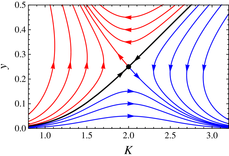
Figure 1: Schematic RG flow near the metal-insulator transition in the symmetry class AIII according to Eqs. (44) and (46).

V.3 Vortex-driven localization

Let us study in more detail the RG equations in class AIII. As was mentioned in the end of Sec. IV, Eqs. (45) and (46) are exact to all orders in the $1/\sigma$ loop expansion. The only assumption used in deriving these equations is $y\ll 1$. Let us neglect this assumption for a moment and treat the RG equations as if they were exact. Another feature of the symmetry class AIII is the partial separation of variables. Renormalization of $K$ and $y$ is independent of $\sigma$. This allows us to study the 2D flow in the $K$ – $y$ plane. The flow is depicted in Fig. 1. The diagram contains one unstable fixed point at the position $K=2$, $y=1/4$. The black line passing through this point separates the two stable phases of the system. Below this line, the flow is directed towards $y=0$ and $K\to\infty$. This part of the diagram corresponds to metallic phase. With vanishing fugacity, renormalization of conductivity stops at some finite value, while the stiffness $K$ keeps increasing solely due to renormalization of the Gade parameter $c$. In the metallic phase, the system rapidly approaches the regime described by the Gade sigma model without vortices. The finite contribution of the dipoles can be included into bare parameters of this sigma model.

Above the critical line, fugacity $y$ increases indefinitely, which signifies vortex unbinding. This phase is analogous to the high-temperature disordered phase in the BKT problem and corresponds to the insulating state of the sample. Indeed, according to Eq. (45), the conductivity flows all the way to zero with growing $y$. Perturbative RG equations rapidly become inaccurate in this limit and cannot be used deep in the insulating phase. Nevertheless, using analogy with the BKT transition, we conclude that the distinction between metal and insulator states is robust.

RG equations (44), (45), and (46) were derived assuming small value of the fugacity (and large value of $\sigma$ in classes CII and BDI). This means that the metal-insulator transition fixed point lies at the border of the applicability region of these RG equations. The theory is not quantitatively controllable in the vicinity of the fixed point but the overall qualitative picture of the RG flow and, in particular, the very presence of the unstable fixed point should be correct. Numerical simulations of electron transport in 2D chiral disordered systems would provide a quantitative estimate of the critical properties of the localization transition.

We have found a fixed point of the metal-insulator transition at $\sigma=0$. This signifies the absence of minimal metallic conductivity in the considered problem. In a realistic disordered chiral system, the bare value of fugacity is related to the Drude conductivity by an exponential law $\ln y\propto-\sigma$. This means that the critical state is achieved when both $y$ and $\sigma$ are of order unity. Hence the Anderson transition will normally happen at $\sigma\sim 1$. The exact critical value of $\sigma$ depends on microscopic details of a particular realization of the disordered system.

In the next section we present an alternative framework for the derivation of non-perturbative renormalization equations for the chiral class AIII. (We expect that a generalization of this approach to other chiral classes is possible as well but it requires further work.)

VI Class AIII and generalized sine-Gordon theory

VI.1 Sigma-model and duality transformation

The group nature of the sigma-model target space for the class AIII allows us to develop yet another description of vortices, bearing analogy with the sine-Gordon theory of the BKT transition.Minnhagen To construct such a description we first work out a dual representation of the AIII sigma model. The inclusion of vortex excitations turns out to be straightforward within this approach.

As a starting remark, let us note that for any field $Q(\mathbf{r})$ of unitary matrices one can define an associated two-component vector field

$$\mathbf{h}=-iQ^{-1}\nabla Q.$$ (47)

The components of $\mathbf{h}$ are Hermitian $N\times N$ matrices. Conversely, given a vector field $\mathbf{h}$ with Hermitian entries and the value of the unitary matrix $Q$ at a single point, one can reconstruct $Q$ in the whole plane by integrating the system of equations

$$\nabla_{\mu}Q=iQh_{\mu}.$$ (48)

The solution of Eq. (48), if exists, is automatically a unitary matrix field. Examining the cross-derivatives of $Q$, we find that the compatibility condition for the system (48) is given by

$$F_{\mu\nu}\equiv\nabla_{\mu}h_{\nu}-\nabla_{\nu}h_{\mu}+i[h_{\mu},h_{\nu}]=0.$$ (49)

Quite remarkably, the integrability constraint (49) can be viewed as a requirement of vanishing field-strength tensor for the non-abelian “gauge field” $\mathbf{h}$.

We thus come to the conclusion that the matrix field $Q$ is in one-to-one correspondence with the vector field $\mathbf{h}$ subject to the integrability constraint (48). In particular, the grand partition function of the sigma model can be represented as

$$Z=\int DQ\,e^{-S[Q]}=\int\left\{\prod_{\mathbf{r}}d^{2}h(\mathbf{r})\,\delta\big{[}F_{xy}(\mathbf{r})\big{]}\right\}e^{-S[\mathbf{h}]},$$ (50)

where the action functional is quadratic in $\mathbf{h}$, cf. Eq. (3):

$$S[\mathbf{h}]=\int\frac{d^{2}r}{8\pi}\left[\sigma\mathop{\mathrm{Tr}}\mathbf{h}^{2}+c\,(\mathop{\mathrm{Tr}}\mathbf{h})^{2}\right].$$ (51)

A straightforward inspection shows that the integration measure over $\mathbf{h}$ in Eq. (50) is indeed flat.

The functional $\delta$-function in Eq. (50) can be resolved by the integration over an auxiliary Hermitian matrix field $\Theta$

$$Z =\int D\mathbf{h}\,D\Theta\,e^{-S[\mathbf{h},\Theta]},$$ (52)

$$S[\mathbf{h},\Theta] =S[\mathbf{h}]+i\int d^{2}r\mathop{\mathrm{Tr}}(\Theta F_{xy}).$$ (53)

Since the action $S[\mathbf{h},\Theta]$ is quadratic in $\mathbf{h}$, we can easily perform the integration over $\mathbf{h}$. As a result, we obtain a dual representation of the AIII sigma model in terms of the matrix $\Theta$:

$$Z =\int D\mu(\Theta)e^{-S[\Theta]},$$ (54)

$$S[\Theta] =\frac{2\pi}{\sigma+Nc}\int d^{2}r\,(\nabla\theta_{0})^{2}$$

$$+\frac{2\pi}{\sigma}(\delta_{\mu\nu}+i\epsilon_{\mu\nu})\int d^{2}r\,(\nabla_{\mu}\theta_{a})g_{ab}(\theta)(\nabla_{\nu}\theta_{b}).$$ (55)

Here we have introduced a decomposition $\Theta=\theta_{0}/\sqrt{N}+\sum_{a=1}^{N^{2}-1}\theta_{a}T^{a}$ of the matrix $\Theta$ over the generators of $\mathrm{U}(N)$. Further, $g_{ab}$ is a $(N^{2}-1)\times(N^{2}-1)$ matrix given by

$$g=\big{(}\mathbbm{1}-4\pi Z/\sigma\big{)}^{-1},\qquad Z_{ab}=\sum_{c=1}^{N^{2}-1}\theta_{c}f_{abc},$$ (56)

where $f_{abc}=-i\mathop{\mathrm{Tr}}T^{a}[T^{b},T^{c}]$ are the structure constants of the $\mathfrak{su}(N)$ algebra. The measure of functional integration over $\Theta$ in (54) is $D\mu(\Theta)=\prod_{\mathbf{r}}\det\{g[\Theta(\mathbf{r})]\}\,d\Theta(\mathbf{r})$. Since $(g+g^{T})/2=gg^{T}$ can be regarded as the metric tensor of the model, we recognize that the integration measure is consistent with the metric.

By construction, the model defined in Eqs. (54), (55) is fully equivalent to the original AIII sigma model. In particular, the two theories should obey identically the same perturbative renormalization group. In Appendix A we verify this fact explicitly within a one-loop calculation.

So far we were completely neglecting the vortex excitations. To include them into the theory, one must realize that integrability condition Eq. (49) can be slightly relaxed. Indeed, as discussed above, a single vortex centered at the origin of the coordinate frame is described by the $Q$ matrix

$$Q=\mathbbm{1}+|p\rangle(e^{i\phi}-1)\langle p|.$$ (57)

Here $\phi$ is the polar angle and $|p\rangle\langle p|$ projects onto some unit vector $|p\rangle$ in the replica space. The corresponding $\mathbf{h}$ field has only the azimuthal component $h_{\phi}=|p\rangle\langle p|/r$ and the field-strength tensor assumes the form

$$F_{xy}(\mathbf{r})=2\pi\delta(\mathbf{r})|p\rangle\langle p|.$$ (58)

A straightforward generalization of Eq. (58) to the case of an arbitrary collection of vortices and anti-vortices located at points $\mathbf{r}_{i}$ and characterized by projectors $|p_{i}\rangle\langle p_{i}|$ reads

$$F_{xy}(\mathbf{r})=2\pi\sum_{i}\eta_{i}\delta(\mathbf{r}-\mathbf{r}_{i})|p_{i}\rangle\langle p_{i}|,\qquad\eta_{i}=\pm 1.$$ (59)

We now repeat the treatment leading to the construction of the dual sigma-model representation (54), (55) but this time taking into account vortex configurations [i.e. replacing the constraint $F_{\mu\nu}=0$ by Eq. (59). This yields

$$Z=\int D\mu(\Theta)e^{-S[\Theta]}\sum_{n=1}^{\infty}\frac{(\Lambda^{2}y_{0})^{n}}{n!}\\ \times\sum_{\eta_{i}=\pm 1}\prod_{i=1}^{n}\int d^{2}r_{i}\,d|p_{i}\rangle\exp[2\pi i\eta_{i}\langle p_{i}|\theta(\mathbf{r}_{i})|p_{i}\rangle]\\ =\int D\mu(\Theta)e^{-S[\Theta]-S_{y}[\Theta]}.$$ (60)

Here $y=e^{-S_{v}}$ is the bare value of fugacity, integration with respect to $|p_{i}\rangle$ is performed over all complex vectors of unit length with natural integration measure, and the vortex-induced correction to the action reads

$$S_{y}[\Theta]\equiv-2y\Lambda^{2}\int d^{2}r\,d|p\rangle\,\cos 2\pi\langle p|\Theta(\mathbf{r})|p\rangle.$$ (61)

The action of the dual theory given by a sum of Eqs. (55) and (61) constitutes the central result of this section. It provides a convenient starting point for the generation of the RG equations (including non-perturbative contributions) for the sigma model of class AIII.

VI.2 RG analysis

We are now in a position to explore the RG flow of the AIII sigma model from the point of view of the dual representation. In the minimal model of class AIII, the $\mathrm{U}(1)$ sigma model, Eqs. (55) and (61) reduce to the standard sine-Gordon action

$$S[\Theta]+S_{y}[\Theta]=\int d^{2}r\left[\frac{2\pi}{\sigma+c}(\nabla\theta_{0})^{2}-2y\Lambda^{2}\cos 2\pi\theta_{0}\right],$$ (62)

and we recover the BKT renormalization group. Let us now explore the contribution of vortices to RG equations in a general situation $N\neq 1$. As in the BKT theory, we will do this perturbatively in the vortex fugacity $y_{0}$. We neglect for a while the non-linear terms in $S[\Theta]$, i.e. replace $S[\theta]$ by

$$S_{0}[\theta]=2\pi\int d^{2}r\left[\frac{(\nabla\theta_{0})^{2}}{\sigma+Nc}+\sum_{a}\frac{(\nabla\theta_{a})^{2}}{\sigma}\right].$$ (63)

Following the standard procedure we decompose the fields $\Theta$ into the fast and slow modes $\Theta=\Theta_{<}+\Theta_{>}$, with the fast modes $\Theta_{>}$ populating a thin shell in momentum space $\Lambda^{\prime}\equiv\Lambda-\Delta\Lambda<|k|<\Lambda$. The action functional becomes

$$S[\Theta_{>}+\Theta_{<}]=S_{0}[\Theta_{<}]+S_{0}[\Theta_{>}]+S_{y}[\Theta_{<}]+S_{1}[\Theta_{<},\Theta_{>}],$$ (64)

where

$$S_{1}[\Theta_{>},\Theta_{<}] =S_{c}[\Theta_{>},\Theta_{<}]+S_{s}[\Theta_{>},\Theta_{<}],$$ (65)

$$S_{c(s)}[\Theta_{>},\Theta_{<}] =-2\Lambda^{2}y\int d^{2}r\,d|p\rangle\,U_{c(s)}(\mathbf{r},|p\rangle),$$ (66)

$$U_{c}(\mathbf{r},|p\rangle) =\big{(}\!\cos 2\pi\langle p|\Theta_{>}(\mathbf{r})|p\rangle-1\big{)}$$

$$\qquad\times\cos 2\pi\langle p|\Theta_{<}(\mathbf{r})|p\rangle,$$ (67)

$$U_{s}(\mathbf{r},|p\rangle) =-\sin 2\pi\langle p|\Theta_{>}(\mathbf{r})|p\rangle\sin 2\pi\langle p|\Theta_{<}(\mathbf{r})|p\rangle.$$ (68)

It is easy to see that to the first order in $y$ the interaction term $S_{1}$ generates the correction to fugacity itself governed by the RG equation [the stiffness parameter $K$ was defined in Eq. (30)]:

$$\frac{\partial y}{\partial\ln\Lambda/\Lambda^{\prime}}=(2-K)y.$$ (69)

We now turn to terms of the second order in fugacity. We observe that, strictly speaking, the action of our model does not preserve its form under the RG transformations. For example, let us consider the contribution to the action due to the interaction $S_{c}$:

$$\Delta S_{c}[\Theta_{<}]=-\frac{1}{2}\big{<}\!\big{<}S_{c}^{2}\big{>}\!\big{>}=-2\Lambda^{4}y^{2}\int d^{2}R\,d^{2}r\,d|p_{1}\rangle\,d|p_{2}\rangle\,\\ \times\big{<}\!\big{<}U_{c}(\mathbf{R}_{+},|p_{1}\rangle)U_{c}(\mathbf{R}_{-},|p_{2}\rangle)\big{>}\!\big{>},$$ (70)

where $\mathbf{R}_{\pm}=\mathbf{R}\pm\mathbf{r}/2$. The gradient expansion of the slow fields leads to

$$\Delta S_{c}[\Theta_{<}]=-\Lambda^{4}y^{2}\int d^{2}R\,d^{2}r\,d|p_{1}\rangle d|p_{2}\rangle\,(X_{+}+X_{-}),\\ \times\big{<}\!\big{<}\cos 2\pi\langle p_{1}|\Theta_{>}(\mathbf{R}_{+})|p_{1}\rangle\cos 2\pi\langle p_{2}|\Theta_{>}(\mathbf{R}_{-})|p_{2}\rangle\big{>}\!\big{>},$$ (71)

with

$$X_{\pm}=\cos 2\pi\big{[}\langle p_{1}|\Theta_{<}(\mathbf{R})|p_{1}\rangle\pm\langle p_{2}|\Theta_{<}(\mathbf{R})|p_{2}\rangle\big{]}\\ \times\left[1\pm\frac{r^{2}}{4}\langle p_{1}|\nabla\Theta_{<}(\mathbf{R})|p_{1}\rangle\langle p_{2}|\nabla\Theta_{<}(\mathbf{R})|p_{2}\rangle\right].$$ (72)

We see that the RG flow generates terms of the form $\cos 2\pi\big{[}\langle p_{1}|\Theta_{<}|p_{1}\rangle\pm\langle p_{2}|\Theta_{<}|p_{2}\rangle\big{]}$ corresponding to the creation of two vortices (for plus sign) or a vortex and anti-vortex (for minus sign) sitting at the same point and characterized by the projectors $|p_{1}\rangle\langle p_{1}|$ and $|p_{2}\rangle\langle p_{2}|$. While the former process is irrelevant in RG sense, the latter one can be even more relevant perturbation than the initial $\cos 2\pi\langle p|\Theta_{<}|p\rangle$ term if vectors $|p_{1}\rangle$ and $|p_{2}\rangle$ are sufficiently close. However, these terms are suppressed by additional power of fugacity $y\ll 1$ as compared to the original vortex term, and we neglect them. Clearly, this neglect is not justified in the region $y\sim 1$ where the fixed point governing the transition is located. At the same time, the theory we are developing is quantitatively controllable only at $y\ll 1$. Discarding the above terms should not lead to any qualitative changes in the RG flow.

We are only interested in the most important $y^{2}$ terms, i.e., those that produce contributions to renormalization of $\sigma$ and $K$ and are thus responsible for the localization transition. To obtain them, we approximate the correction (71) to the action of the slow fields by

$$\Delta S_{c}[\Theta_{<}]=2\pi\kappa\Lambda^{4}y^{2}\int d^{2}R\,d|p\rangle\,\langle p|\nabla\Theta_{<}(R)|p\rangle^{2}\\ \times\!\!\int\!\!d^{2}r\,r^{2}\,\big{<}\!\big{<}\!\cos 2\pi\langle p|\Theta_{>}(\mathbf{R}_{+})|p\rangle\cos 2\pi\langle p|\Theta_{>}(\mathbf{R}_{-})|p\rangle\big{>}\!\big{>}.$$ (73)

Here $\kappa$ is a numerical coefficient. Averaging now over the fast fields and singling out the contributions of the first order in $\Delta\Lambda$ we get

$$\Delta S_{c}[\Theta_{<}]=2\pi\kappa\frac{\Delta\Lambda}{\Lambda}K^{2}y^{2}\int d^{2}R\,d|p\rangle\,\langle p|\nabla\Theta_{<}(\mathbf{R})|p\rangle^{2}.$$ (74)

(We have absorbed an additional numerical coefficient into $\kappa$.) Noting that for arbitrary matrices $A$ and $B$

$$\int d|p\rangle\langle p|A|p\rangle\langle p|B|p\rangle=\frac{V_{p}}{N(N+1)}\big{(}\mathop{\mathrm{Tr}}A\mathop{\mathrm{Tr}}B+\mathop{\mathrm{Tr}}AB\big{)},$$ (75)

we finally get

$$\Delta S_{c}[\Theta_{<}]=2\pi\kappa\frac{\Delta\Lambda}{\Lambda}\frac{V_{p}}{N(N+1)}K^{2}y^{2}\\ \times\left[(n+1)(\nabla\theta^{0}_{<})^{2}+\sum_{a=1}^{N^{2}-1}(\nabla\theta^{a}_{<})^{2}\right].$$ (76)

Comparing now Eq. (76) with the Gaussian action (63), we conclude that integration over the fast modes has generated corrections to $\sigma$ and $c$ given by

$$\Delta\sigma =-\kappa\frac{y^{2}K^{2}\sigma^{2}}{\Gamma(N+2)}\frac{\Delta\Lambda}{\Lambda},$$ (77)

$$\Delta c =-\kappa\frac{y^{2}K^{2}}{\Gamma(N+1)}\frac{\Delta\Lambda}{\Lambda}\left[\frac{\sigma^{2}}{N+1}+2\sigma c+Nc^{2}\right].$$ (78)

So far we were neglecting non-Gaussian terms in the action $S[\Theta]$. When taken into account, they will induce the perturbative renormalization of the parameters of the model and, in particular, lead to the appearance of the scale-dependent $\sigma$ and $c$ in Eqs. (77) and (78). Apart from this, the higher order terms do not affect our analysis: a straightforward calculation shows that in our approximation the interaction term $\Delta S_{s}$ does not produce corrections of order $y^{2}$. Combining Eqs. (69), (77), and (78), we obtain a system of RG equations for the AIII sigma model

$$\frac{\partial\sigma}{\partial\ln L} =-N-\frac{y^{2}K^{2}\sigma^{2}}{\Gamma(N+2)},$$ (79)

$$\frac{\partial K}{\partial\ln L} =\frac{1-N}{4}-\frac{y^{2}K^{2}}{\Gamma(N+1)}\left(\frac{2\sigma^{2}}{N+1}+2\sigma c+Nc^{2}\right),$$ (80)

$$\frac{\partial y}{\partial\ln L} =(2-K)y.$$ (81)

These equations are equivalent to those obtained in Sec. V up to subleading terms. To make this equivalence apparent, we redefine the fugacity parameter according to $y\mapsto(y/K)\sqrt{\Gamma(N+1)/\sigma}$. This amounts to changing the (uncontrolled) pre-exponential factor in the exponentially small quantity $y$. After such a rescaling, the RG equations (42), (43), and (44) are reproduced.

VII Topological terms

In previous sections, we discussed localization within the Gade-Wegner sigma model, Eq. (3), of three chiral classes. Now we will consider the situations when the sigma-model action is augmented with an additional topological term. The topology of the sigma-model target spaces allows (in two dimensions) inclusion of the Wess-Zumino term in class AIII and the $\mathbb{Z}_{2}$ $\theta$ term in class CII. We will demonstrate below that these extra terms (arising in models of random Dirac fermions of the corresponding symmetries) crucially affect localization properties. Specifically, we show that vortex excitations do not appear when a topological term is present.

VII.1 Class AIII with Wess-Zumino term

The field of the sigma model of class AIII is a unitary matrix $Q(\mathbf{r})\in\mathrm{U}(N)$, with $\mathbf{r}$ belonging to the 2D coordinate space. In our analysis we consider only field configurations with the $Q$ matrix taking some fixed value at spatial infinity. (Otherwise the sigma-model action inevitably diverges due to gradient terms.) This allows us to compactify the coordinate space making it equivalent to a two-sphere. The compactified real space $S^{2}$ can be viewed as a surface of a three-dimensional solid ball and we introduce the radial coordinate $\tau$ such that $\tau=1$ at the surface (i.e., in the physical 2D space) and $\tau=0$ in the center of the ball. The matrix $Q$ can be continuously extended to the interior of the ball such that

$$Q(\mathbf{r},\tau)=\begin{cases}Q(\mathbf{r}),&\tau=1,\\ \mathop{\mathrm{const}},&\tau=0.\end{cases}$$ (82)

This extension is always possible since the second homotopy group of the target space is trivial, $\pi_{2}(U)=0$.

In terms of the extended matrix $Q(\tau)$, the Wess-Zumino term acquires the form

$$S_{\text{WZ}}[Q]=\frac{ik}{12\pi}\,\epsilon_{\mu\nu\lambda}\\ \times\int d\tau\,d^{2}r\mathop{\mathrm{Tr}}\Big{(}Q^{-1}\nabla_{\mu}QQ^{-1}\nabla_{\nu}QQ^{-1}\nabla_{\lambda}Q\Big{)}.$$ (83)

The integrand in this expression explicitly depends on the values of $Q$ at $\tau\neq 1$, i.e., away from the physical 2D space. However, the variation of the Wess-Zumino action can be represented as an integral of a three-dimensional vector divergence:

$$\delta S_{\text{WZ}}[Q]=\frac{ik}{4\pi}\,\epsilon_{\mu\nu\lambda}\\ \times\int d\tau\,d^{2}r\nabla_{\mu}\mathop{\mathrm{Tr}}\Big{(}Q^{-1}\delta QQ^{-1}\nabla_{\nu}QQ^{-1}\nabla_{\lambda}Q\Big{)}\\ =\frac{ik}{4\pi}\int d^{2}r\mathop{\mathrm{Tr}}\Big{(}Q^{-1}\delta Q\big{[}Q^{-1}\nabla_{x}Q,Q^{-1}\nabla_{y}Q\big{]}\Big{)}.$$ (84)

Thus the actual value of the Wess-Zumino term is determined only by the physical values of $Q$ at $\tau=1$ up to a constant. This constant does not change with small variations of $Q$ away from the physical 2D space but takes different values for topologically distinct extensions of $Q$ in the third dimension. These nonequivalent extensions are classified by the third homotopy group $\pi_{3}(U)=\mathbb{Z}$. For any two extensions the values of the Wess-Zumino term differ by $2\pi ik$ times an integer number. Thus the Wess-Zumino theory is well-defined for any integer value of $k$.

Introducing vortices in the Wess-Zumino theory is problematic. In order to avoid the singularity in the center of a vortex, we exclude a small region of the vortex core from our physical space. This introduces a boundary in the problem and $Q$ is not a constant along this boundary. As a result, the 2D physical space cannot be compactified to the two-sphere. Thus the construction of the Wess-Zumino term, involving extension to the third dimension, becomes ill-defined.

One naive way to overcome this difficulty is to use a local 2D representation of the Wess-Zumino term.Witten As was discussed above, the Wess-Zumino term actually depends only on the values of $Q$ in the physical space. Using any explicit parameterization of the unitary matrix $Q$ by a set of coordinates $\psi_{i}$, the Wess-Zumino term can be written as a 2D integral of a suitable skew-symmetric differential form $\lambda_{ij}$:

$$S_{\text{WZ}}[Q]=ik\,\epsilon_{\mu\nu}\int d^{2}r\;\lambda_{ij}\big{[}\psi(\mathbf{r})\big{]}\nabla_{\mu}\psi_{i}\nabla_{\nu}\psi_{j}.$$ (85)

In this local representation, one can integrate the differential form over a finite physical space with boundary. Such a construction is however unsatisfactory because it violates the global gauge symmetry of the system. Indeed, the Wess-Zumino action (83) is manifestly invariant under the global transformation $Q\mapsto U_{L}QU_{R}$ parameterized by two constant unitary matrices $U_{L,R}$. However, the local density of the Wess-Zumino term, Eq. (85), is not invariant under global rotation of fields. Instead, the tensor $\lambda_{ij}$ transforms as

$$\lambda_{ij}\mapsto\lambda_{ij}+\frac{\partial\beta_{j}}{\partial\psi_{i}}-\frac{\partial\beta_{i}}{\partial\psi_{j}}$$ (86)

where a set of functions $\beta(\psi)$ encodes the information about $U_{L}$ and $U_{R}$. The local expression for the Wess-Zumino term changes by an integral of a total derivative:

$$S_{\text{WZ}}\mapsto S_{\text{WZ}}+2ik\,\epsilon_{\mu\nu}\int d^{2}r\;\nabla_{\mu}(\beta_{j}\nabla_{\nu}\psi_{j}).$$ (87)

If the model is considered on a manifold without a boundary, the above integral vanishes and the Wess-Zumino term is indeed invariant under the gauge transformation. If, however, the real space integration is performed over a bounded region, the integral in Eq. (87) yields the circulation of $\beta_{j}\nabla\psi_{j}$ along the boundary and may become non-zero. This signifies the breakdown of the gauge symmetry at the boundary.

In order to understand better the boundary effects in the Wess-Zumino theory, we will resort to the disordered fermion problem yielding the class AIII sigma model with the Wess-Zumino term. The typical example is given by disordered massless Dirac fermions with random vector potential. The Hamiltonian of such a model has the form

$$H=\begin{pmatrix}0&p_{x}-ip_{y}+a\\ p_{x}+ip_{y}+a^{\dagger}\end{pmatrix}.$$ (88)

Here $a$ is a random complex-valued matrix acting in the auxiliary flavor space. The only symmetry of the Hamiltonian is the chiral symmetry $H=-\sigma_{z}H\sigma_{z}$. Since the spectrum of the Hamiltonian is unbounded, it appears to be impossible to introduce the boundary condition (a classically forbidden region for massless Dirac fermions) preserving the chiral symmetry. In order to model a hole in the sample, one has to add an additional mass term $m\sigma_{z}$ to the Hamiltonian and consider the limit of large $m$. Such a term explicitly breaks the chiral symmetry. In the corresponding sigma model, the $Q$ matrix at the hole boundary will be restricted to the manifold $\mathcal{M}_{A}=\mathrm{U}(N)/\mathrm{U}(N/2)\times\mathrm{U}(N/2)$ of class A. Such a boundary condition will maintain only the diagonal part of the global gauge symmetry $U_{L}=U_{R}^{-1}$. This also forbids the vortex excitations inside the hole since $\mathcal{M}_{A}$ is simply connected. Thus we see that the short distance regularization (making a small hole), needed to introduce a vortex in the sigma model, breaks the chiral symmetry and does not allow a vortex excitation. We conclude that vortices are incompatible with the Wess-Zumino term in the action of class AIII.

The model of massless Dirac fermions in a random magnetic field, described by the Hamiltonian (88) is exactly solvable. The coupling constant characterizing the vector potential strength is exactly marginal, so that the model possess a line of fixed points. A remarkable property of this problem is that the system never gets truly localized, however strong the disorder is. In particular, the conductivity is equal to $e^{2}/\pi h$ for any disorder. Therefore, the absence of the localizing vortex contribution in the corresponding sigma-model is consistent with the known exact solution of the underlying fermionic problem.

Let us illustrate the incompatibility of vortices and Wess-Zumino term in a more explicit way. We will construct an extension of the sigma-model manifold such that the theory will be well-defined inside the vortex core while all the symmetries are preserved. Let us extend the $Q$ matrix by one row and one column embedding $\mathrm{U}(N)$ into $\mathrm{SU}(N+1)$. We will associate a mass $M$ with the extra degrees of freedom suppressing them away from a vortex core. Explicitly, consider the following action for the extended unitary matrix $\underline{Q}$:

$$S[\underline{Q}]=-\int\frac{d^{2}r}{8\pi}\Bigg{[}\sigma\mathop{\mathrm{Tr}}(\underline{Q}^{-1}\nabla\underline{Q})^{2}+M^{2}\mathop{\mathrm{Tr}}(\underline{Q}R\underline{Q}^{-1}R)\\ +\frac{c-\sigma}{4}(\mathop{\mathrm{Tr}}R\underline{Q}^{-1}\nabla\underline{Q})^{2}\Bigg{]}+S_{\text{WZ}}[\underline{Q}].$$ (89)

Here the matrix $R$ of the form

$$R=\begin{pmatrix}-1&0\\ 0&\mathbbm{1}_{N\times N}\end{pmatrix}$$ (90)

is introduced to single out the off-diagonal elements in the first row and first column of $\underline{Q}$. These elements are made massive by the second term of the action (89).

Away from vortices the matrix $\underline{Q}$ contains only the soft modes arranged as follows:

$$\underline{Q}_{\text{soft}}=\begin{pmatrix}\det Q^{-1}&0\\ 0&Q\end{pmatrix}.$$ (91)

The lower right diagonal block is nothing but the unitary matrix $Q$ while the upper left diagonal element is fixed such that $\det\underline{Q}=1$. With such a form of $\underline{Q}$, the action (89) coincides with the standard AIII class sigma-model action (3) with a Wess-Zumino term added. At the same time, the group $\mathrm{SU}(N+1)$ is simply connected hence the vortices are topologically trivial configurations in the extended model. Inside a vortex core, massive elements of $\underline{Q}$ become non-zero and provide an overall smooth field configuration. The size of the core is determined by the competition between energy loss due to the mass $M$ and energy gain due to avoiding large gradients. This yields the core size $\sim\sqrt{\sigma}/M$.

Within the extended model we can examine the inner structure of the vortex core. Assume for simplicity that the vortex occurs in the first replica, i.e., the corresponding unit vector is $|p\rangle=\{1,0,\dots,0\}$. The whole vortex configuration, including the core, will involve only the upper-left $2\times 2$ block of the matrix $\underline{Q}$. This block is an $\mathrm{SU}(2)$ matrix and we can explicitly parameterize it by three angles in the following way:

$$\underline{Q}=\begin{pmatrix}\cos\theta e^{-i\phi}&i\sin\theta e^{-i\chi}&0\\ i\sin\theta e^{i\chi}&\cos\theta e^{i\phi}&0\\ 0&0&\mathbbm{1}_{N-1\times N-1}\end{pmatrix}.$$ (92)

Far from the vortex core, the angle $\theta$ vanishes and the matrix $\underline{Q}$ acquires the form (91); it is independent of $\chi$. Going around the vortex, angle $\phi$ rotates by $2\pi$. In the center of the vortex $\theta=\pi/2$ and $\underline{Q}$ is independent of $\phi$ but explicitly depends on $\chi$. Using the ansatz (92), we can minimize the action (89). The symmetry of vortex allows us to fix parameter $\phi$ equal to the polar angle and $\chi$ constant. We see that the vortex core acquires an inner $\mathrm{U}(1)$ degree of freedom, $\chi$, which is beyond the sigma model and is effective only in the extended theory. The action is minimized by a proper $\theta(r)$ dependence.

The Wess-Zumino term is responsible for the imaginary part of the action. We can calculate this imaginary part without solving for $\theta(r)$ dependence. Let us consider the variation of the Wess-Zumino term with respect to spatially constant $\chi$. Upon substitution of Eq. (92) into Eq. (84), we obtain

$$\delta S_{\text{WZ}}[\underline{Q}]=\frac{ik\delta\chi}{2\pi}\int d^{2}r\,\sin 2\theta\big{(}\nabla_{x}\theta\nabla_{y}\phi-\nabla_{y}\theta\nabla_{x}\phi\big{)}\\ =ik\delta\chi\Big{[}\sin^{2}\theta(r=\infty)-\sin^{2}\theta(r=0)\Big{]}=-ik\delta\chi.$$ (93)

Thus the value of the Wess-Zumino term explicitly depends on $\chi$.

The imaginary part of the action makes vortex fugacity complex. The arameter $\chi$, that determines the phase of the complex fugacity, is an internal degree of freedom of the vortex core. Calculating the partition function of the system, we have to integrate over $\chi$ for each vortex. Once the action contains the Wess-Zumino term, i.e., $k\neq 0$, such an integration will exactly cancel the statistical weight of each vortex making fugacity effectively zero. This once again demonstrates that the Wess-Zumino model of class AIII does not allow vortex excitations.

VII.2 Class CII with $\mathbb{Z}_{2}$ $\theta$ term

Let us now consider the system of symmetry class CII. The topology of the target manifold admits the $\mathbb{Z}_{2}$ topological term. It is related to the homotopy group $\pi_{2}(\mathrm{U}(N)/\mathrm{O}(N))=\mathbb{Z}_{2}$. One particular realization of the symmetry class CII is provided by the disordered massless Dirac Hamiltonian of the form Eq. (1) with

$$h=\begin{pmatrix}p_{x}-ip_{y}&a\\ -a^{*}&p_{x}+ip_{y}\end{pmatrix}.$$ (94)

Here $a$ is a random $n\times n$ matrix with complex entries. The block $h$ obeys symplectic constraint $h^{*}=\tau_{y}h\tau_{y}$. In other words, $h$ is an $n\times n$ matrix of real quaternions. Thus the Hamiltonian built from $h$ indeed belongs to the symmetry class CII.

The derivation of the sigma model for the disordered system described by the Hamiltonian (1), (94) is outlined in Appendix B. The action of the model has the standard form (3) with an additional $\mathbb{Z}_{2}$ topological term when $n$ is odd. This topological term can be expressed in the form very similar to the Wess-Zumino term (83). Specifically, we have to continuously extend the $Q$ matrix to the auxiliary third dimension $\tau$ according to Eq. (82). Then the topological term can be written in the form of Eq. (83) with $k=n$. Since the second homotopy group of the target manifold is non-trivial, the extension (82) is not always possible within the target space of class CII. In fact, it is only possible for topologically trivial configurations of $Q(\mathbf{r})$. To apply the Wess-Zumino construction to a general field configuration, we will assume that away from the physical 2D space, at $\tau\neq 1$, $Q$ is any unrestricted unitary matrix from $\mathrm{U}(N)$, while for $\tau=1$ it is unitary and symmetric hence belongs to the coset space $\mathrm{U}(N)/\mathrm{O}(N)$ of the class CII.

Similarly to the class AIII, the value of the Wess-Zumino term is actually determined by the physical part of $Q$ at $\tau=1$ which is a unitary symmetric matrix. The variation of the Wess-Zumino term with small variations of $Q$ is given by Eq. (84). Using the property $Q=Q^{T}$ and transposing the argument of the trace in the last line of Eq. (84), we see that the variation changes sign and hence is identically zero. This proves that such a Wess-Zumino term in the class CII possesses the main property of the theta term: it depends only on the topology of the field configuration.

Apart from the class of topologically trivial configurations, there is only one extra non-trivial class. In other words, the homotopy group $\pi_{2}=\mathbbm{Z}_{2}$ implies existence of localized topological “excitations”, $\mathbbm{Z}_{2}$ instantons. They are their own “antiparticles”; configuration of two such instantons is topologically trivial, i.e. the instantons can be brought close to each other and annihilated by an appropriate continuous transformation of $Q$. In order to prove that the Wess-Zumino term (83), being constant in each topological class, distinguishes between them, it suffices to evaluate it for one particular non-trivial instanton configuration.

Let us consider the minimal model $Q\in\mathrm{U}(2)/\mathrm{O}(2)$. (In fact, in this case the homotopy group $\pi_{2}=\mathbb{Z}$ is reacher than in the general case $N>2$ and the theory possesses usual $\mathbb{Z}$ instantons similar to, e.g., $\mathrm{O}(3)$ vector sigma model.) In fact, it is sufficient to consider an even smaller target space $\mathrm{SU}(2)/\mathrm{O}(2)$ since the determinant of $Q$ anyway drops from the Wess-Zumino term (83). We parametrize the $\mathrm{SU}(2)$ matrix by three angles in the following way:

$$Q=\begin{pmatrix}\cos\theta\cos\chi e^{-i\phi}&i\sin\theta\cos\chi+\sin\chi\\ i\sin\theta\cos\chi-\sin\chi&\cos\theta\cos\chi e^{i\phi}\end{pmatrix}.$$ (95)

The symmetry condition $Q=Q^{T}$ fixes $\chi=0$ in the physical 2D space. For the instanton, we can assume that $\phi$ is equal to the polar angle while $\theta$ depends only on the radial coordinate and changes continuously from $-\pi/2$ in the center of the instanton to $\pi/2$ at infinity. Extending to the third dimension, we will assume $\chi$ to change from $0$ at $\tau=1$ to either $\pi/2$ or $-\pi/2$ at $\tau=0$. Any of these two values uniquely fixes the whole matrix $Q(\tau=0)$.

Wess-Zumino action (83) can be explicitly written in the parametrization (95) as

$$S_{\text{WZ}}[Q]=\frac{ik}{\pi}\epsilon_{\mu\nu\lambda}\int d^{2}r\,d\tau\cos\theta\cos^{2}\chi\nabla_{\mu}\theta\nabla_{\nu}\phi\nabla_{\lambda}\chi.$$ (96)

For the instanton configuration, $\theta$ and $\chi$ depend on $r$ and $\tau$, respectively, while $\phi$ is the polar angle. Calculating the integral, we obtain

$$S_{\text{WZ}}[Q]=\mp\frac{i\pi k}{2}\Big{[}\sin\theta(r=\infty)-\sin\theta(r=0)\Big{]}=\mp i\pi k.$$ (97)

The two signs in this expression correspond to the two extensions $\chi(\tau=0)=\pm\pi/2$. For an odd value of $k$, the instanton action acquires a non-trivial imaginary contribution. Thus the Wess-Zumino term indeed plays the role of a theta term yielding $i\pi k$ times the topological charge of the field configuration.

Once the explicit form of the $\mathbb{Z}_{2}$ topological term is established, we can discuss its interplay with vortices. We have already argued that the Wess-Zumino term in the sigma model of class AIII makes vortex excitations ineffective. Similar arguments can be applied to the class CII with the topological term since it has the same structure as the Wess-Zumino term. The only difference in the class CII is an additional constraint related to the time-reversal symmetry. Namely, the statistical weight of any field configuration of the class CII sigma model must be real. Equivalently, the imaginary part of the sigma-model action must be an integer multiple of $i\pi$. It is the topological term that provides this imaginary part. Consider an extension of the model from $\mathrm{U}(N)/\mathrm{O}(N)$ up to $\mathrm{SU}(N+1)/\mathrm{O}(N+1)$. Such an extension is given by, e.g., Eq. (89) with an additional symmetry constraint $\underline{Q}=\underline{Q}^{T}$. The vortex configuration in this extended model has the form Eq. (92) with the angle $\chi$ taking either $0$ or $\pi$ value. Thus the internal $\mathrm{U}(1)$ parameter associated with the vortex in the symmetry class AIII becomes a $\mathbb{Z}_{2}$ degree of freedom in the class CII. The two vortex configurations with $\chi=0$ and $\chi=\pi$ differ by an $i\pi$ term in the action, cf. Eq. (93). Thus summation over the two values of this internal degree of freedom effectively annihilates vortex contribution to the partition function of the system.

The above discussion is based on the specific form of the extended model (89) describing the vortex core. In fact, we can lift this restriction and show that a vortex possesses an internal $\mathbb{Z}_{2}$ degree of freedom without assuming any particular structure of its core. Consider a vortex configuration in the class CII sigma model. We suppose that some additional massive degrees of freedom become relevant in the center of the vortex and once they are taken into account the field configuration is continuous. The extended model must possess the time-reversal symmetry characteristic for the class CII. Hence the statistical weight in the extended model is real and the action is real up to an integer multiple of $i\pi$. Let us now create a small instanton far from the vortex center. This will change the imaginary part of the action by $\pi$. Within the extended theory, we can bring the instanton close to the vortex center and “hide” it inside the core by a continuous field transformation. Since the imaginary part of the action takes only discrete values, this transformation will not remove an extra $i\pi$ from the action related to the instanton. We have thus demonstrated the existence of two topologically distinct vortex solutions in the extended theory with opposite signs of their statistical weights. Since there is no other general distinction between these two solutions, the real parts of their action must be equal. This once again shows that the total statistical weight of a vortex configuration is zero if the underlying sigma model contains the $\mathbb{Z}_{2}$ topological term.

To conclude, additional topological terms in the sigma model of both AIII and CII symmetry classes suppress formation of vortices and thus prevent the system from localization.

VIII Summary and outlook

In this paper, we have developed a field-theoretical (sigma-model) approach to Anderson localization in 2D disordered systems of chiral symmetry classes (AIII, BDI, CII). A remarkable feature of sigma models for these classes is that the quantum interference effects leading to renormalization of conductivity (and thus to Anderson localization) are absent to all orders of perturbation theory. We have shown that Anderson localization does exist within these models and is governed by a non-perturbative mechanism. Specifically, the localization is due to topological excitations – vortices – of the sigma model field. We have derived the corresponding renormalization group equations which include non-perturbative contributions. Analyzing them, we find that the 2D disordered systems of chiral classes undergo a metal-insulator transition driven by topologically induced Anderson localization.

While the mechanism of the localization transition — proliferation of vortices — bears an analogy with the Berezinskii-Kosterlitz-Thouless transition in systems with $\mathrm{U}(1)$ symmetry, our RG equations are essentially different. The reason for this is a more complex structure of the theory: it is characterized by three coupling constants (conductivity $\sigma$, Gade coupling $c$, and fugacity $y$) instead of two couplings of the BKT transition theory (spin stiffness and fugacity). As a result, the fixed point governing the transition turns out to be at non-zero fugacity. For this reason, the critical behavior at the transition cannot be determined in a controllable way. The one-loop analysis suggests that this behavior is of power-law type (i.e. is more similar to the critical behavior at Anderson transitions in conventional classes rather than to that at BKT transition).

For the chiral unitary class AIII, we have presented an alternative derivation of the renormalization group based on a mapping of the sigma model onto a dual theory. The latter has the form of a generalized sine-Gordon theory.

We have also considered 2D disordered systems formed on surfaces of 3D topological insulators of chiral symmetry classes AIII and CII. In this case the sigma model is supplemented by a term of topological origin: the Wess-Zumino term for the class AIII and $\mathbb{Z}_{2}$ theta term for the class CII. We have shown that such terms overpower the effect of vortices, thus ensuring the protection of surface states against the vortex-induced Anderson localization.

Our work opens perspectives for research in a number of important directions. Below, we briefly discuss several of them.

First, it would be very interesting to investigate the metal-insulator transition in chiral classes and the associated critical behavior numerically. Remarkably, this issue is almost unexplored by now. This is in stark contrast with conventional symmetry classes (i.e., symplectic class metal-insulator transition and unitary class quantum Hall transition in 2D, orthogonal class transition in 3D etc.) where very detailed studies have been carried out. Since we are dealing here with non-interacting systems in a relatively low (2D) dimensionality, a sufficiently accurate numerical analysis is expected to be feasible. It would be also interesting to simulate the sigma model directly. This would allow to verify the importance of topological excitations for localization and to test our predictions. Such an approach can be implemented within supersymmetric version of the sigma model with Grassmann degrees of freedom integrated out.Disertori

Second, it remains to develop a dual, sine-Gordon-like theory of the transition, analogous to that presented in Sec. VI for class AIII, for the other two chiral classes. Furthermore, we feel that geometric aspects of sigma-model renormalization within this dual formalism deserve a more thorough investigation.

Third, a natural question arises concerning the metal-insulator transitions in chiral classes in 3D (and higher dimensionalities). We expect that also there the transition will be driven by topological excitations, namely, vortex lines.

Fourth, in analogy with $\mathbb{Z}$ vortices studied above, 2D sigma models of two classes, AII and DIII, allow for $\mathbb{Z}_{2}$ vortices. The difference is that these two classes do show quantum interference effects on the perturbative level. Therefore, in contrast to the chiral classes, the vortices in classes AII and DIII will not constitute the only driving mechanism of Anderson localization but rather will contribute to renormalization of conductivity along with perturbative terms.

Fifth, interaction effects play an important role in low-dimensional systems and may strongly affect the nature of the metal-insulator transition. Two-dimensional Dirac fermions subjected to short-range interaction exhibit the Mott transitionFosterLudwig unlike the non-interacting case when the system remains metallic. It would be very interesting to investigate the interplay of interaction and vortices in systems with chiral symmetry.

Finally, we close with a more general comment. The importance of topological aspects of field theories of disordered systems was recently emphasized in the context of topological insulators SchnyderKitaev ; AL50 . There, a possibility of emergence of a Wess-Zumino term or $\mathbb{Z}_{2}$ theta term in the corresponding dimensionality and symmetry class signals the existence of a topological insulator phase. There is at present a growing appreciation of the fact that the topological properties of sigma-model manifolds may crucially affect the physical observables even for those combinations of dimensionalities and symmetries than do not allow for topological insulators. In particular, a recent work Gruzberg11 has shown that a particular symmetry of local density of states distributions holds for sigma models (and thus for critical points) of five symmetry classes (A, AI, AII, C, CI) but dos not hold for the remaining five (AIII, BDI, CII, D, DIII). The distinct feature of the latter five classes is the presence of $\mathrm{U}(1)$ or $\mathrm{O}(1)$ subgroup in the sigma model target space $\mathcal{M}$ leading to a non-trivial topology: $\pi_{1}(\mathcal{M})=\mathbb{Z}$ for chiral classes (AIII, BDI, CII) and $\pi_{0}(\mathcal{M})=\mathbb{Z}_{2}$ for Bogoliubov-de Gennes classes D and DIII. It is worth emphasizing that these topologies render these five classes topological insulators in 1D. Equivalently, models of these symmetry classes may support eigenstates with exactly zero energies Ivanov02 . As the paper Ref. Gruzberg11, showed, the same $\mathrm{U}(1)$ and $\mathrm{O}(1)$ degrees of freedom that are responsible for topological insulator properties in 1D in fact crucially affect the multifractal spectra at higher dimensionalities. The present work shows that the $\mathrm{U}(1)$ topology of sigma-model manifolds of chiral classes is also responsible for Anderson localization in these classes in 2D (and likely also in higher dimensions). Earlier, the authors of Ref. Bocquet00, argued that the $\mathrm{O}(1)=\mathbb{Z}_{2}$ degree of freedom of the sigma model is responsible for localization in class D in two dimensions. Thus, it turns out that the importance of topological aspects of field theories of disordered systems goes well beyond that expected on the basis of classification of topological insulators. Full ramifications of these observations remain to be understood.

IX Acknowledgments

We are grateful to I. V. Gornyi, I. A. Gruzberg, V. Gurarie, D. A. Ivanov, A. W. W. Ludwig, and M. A. Skvortsov for valuable discussions. The work was supported by the Center for Functional Nanostructures and the SPP 1459 “Graphene” of the Deutsche Forschungsgemeinschaft and by the German Ministry for Education and Research (BMBF). The work of I. V. P. was supported by Alexander von Humboldt Foundation. P. M. O. and A. D. M. acknowledge the hospitality of KITP Santa Barbara at the stage of preparation of the manuscript for publication.

Appendix A Perturbative renormalization in dual representation

The purpose of this appendix is to illustrate the equivalence of the model (54), (55) to the original AIII sigma model by a one-loop perturbative renormalization. Within this calculation we can ignore the Gaussian field $\theta_{0}$ in Eq. (55) (since renormalization of this sector is trivial on the perturbative level) and concentrate on the renormalization of the non-abelian sector of the theory parametrized by fields $\theta_{a}$ with $a=1,\ldots N^{2}-1$. To make more explicit the possibility of a loop expansion controlled by the parameter $\sigma\gg 1$, it is also convenient to rescale $\theta_{a}$ by a factor $\sigma/4\pi$. The action of the model acquires now the form

$$S[\theta]=\frac{\sigma}{8\pi}\big{(}\delta_{\mu\nu}+i\epsilon_{\mu\nu}\big{)}\int d^{2}r\,(\nabla_{\mu}\theta_{a})g_{ab}(\theta)(\nabla_{\nu}\theta_{b}),$$ (98)

$$g(\theta)=\big{[}\mathbbm{1}-Z(\theta)\big{]}^{-1},\qquad Z_{ab}(\theta)=\sum_{c=1}^{N^{2}-1}\theta_{c}f_{abc}.$$ (99)

The renormalization of the theory can now be carried out in the standard manner. We split the fields $\theta^{a}$ into the fast and slow components, $\theta=\theta_{<}+\tilde{\theta}_{>}$. We should then expand in the fast fields up to the second order and integrate them out. It proves convenient to perform the change of fast variables $\theta_{>}=g(\theta_{<})\tilde{\theta}_{>}$ so that the decomposition of $\theta$ into the fast and slow fields reads

$$\theta=\theta_{<}+\big{(}1-Z_{<}\big{)}\theta_{>}.$$ (100)

Here we introduced for notational brevity $Z_{<}\equiv Z(\theta_{<})$. This change of integration variables cancels the contribution of the non-trivial integration measure $D\mu(\theta)$ to the renormalization group equations and guarantees the absence of linearly diverging diagrams in one-loop calculation. Denoting also $Z(\theta_{>})$ by $Z_{>}$ we have

$$\nabla\theta =(1+Z_{>})\nabla\theta_{<}+(1-Z_{<})\nabla\theta_{>},$$ (101)

$$Z(\theta) =Z_{<}+Z_{>}+[Z_{>},Z_{<}],$$ (102)

This implies that the quadratic-in-$\theta_{>}$ contribution to the action reads $S_{2}=S_{2}^{(0)}+\delta S_{2}$,

$$S_{2}^{(0)} =\frac{\sigma}{8\pi}\int d^{2}r\,\nabla\theta_{>}^{T}\nabla\theta_{>},$$ (103)

$$\delta S_{2} =\frac{\sigma(\delta_{\mu\nu}+i\epsilon_{\mu\nu})}{8\pi}\int d^{2}r\,\big{[}\nabla_{\mu}\theta_{>}^{T}(1+Z_{<})+\nabla_{\mu}\theta_{<}^{T}g_{<}Z_{>}Z_{<}\big{]}\big{[}\nabla_{\nu}\theta_{>}+g_{<}(2-Z_{<})Z_{>}g_{<}\nabla_{\nu}\theta_{<}\big{]}-S_{2}^{(0)}.$$ (104)

Performing now the expansion in $\delta S_{2}$, averaging over fast fluctuations, and retaining only the logarithmically diverging contributions, we find the correction to the action functional of the slow fields:

$$\Delta S=\frac{N}{8\pi}\ln\frac{\Lambda}{\Lambda^{\prime}}(\delta_{\mu\nu}+i\epsilon_{\mu\nu})\\ \times\int d^{2}r\,\nabla_{\mu}\theta^{T}_{<}\big{[}2g+3g^{2}\big{]}\nabla_{\nu}\theta_{<}\,.$$ (105)

We can recast the action for the slow fields into the original form by correcting the conductivity $\sigma\mapsto\tilde{\sigma}$ and switching to the rescaled filed $\tilde{\theta}$

$$\tilde{\sigma} =\sigma\left(1-\frac{N}{\sigma}\ln\frac{\Lambda}{\Lambda^{\prime}}\right),$$ (106)

$$\tilde{\theta} =\theta\left(1+\frac{3N}{\sigma}\ln\frac{\Lambda}{\Lambda^{\prime}}\right).$$ (107)

(Note that, after the rescaling, the factor $1/(1-Z)$ should be expanded to the first order in $1/\sigma$, which is the accuracy of the one-loop calculation.) We see now that the dual model defined by Eqs. (54), (55) reproduces the correct renormalization of the conductivity $\sigma$.

Appendix B Chiral sigma model for massless Dirac fermions

In this Appendix we outline the derivation of the sigma models for the massless Dirac Hamiltonians of AIII and CII symmetries. Apart from demonstrating the consequences of the chiral symmetry in the sigma-model language, we will also discuss possible topological terms. Such terms frequently appear due to chiral anomaly of the massless Dirac electrons.

B.1 Class AIII

Let us first consider the AIII symmetry class. A general chiral Hamiltonian has the block off-diagonal structure (1). We consider the following Dirac Hamiltonian of AIII symmetry [cf. Eq. (88)]:

$$H=\begin{pmatrix}0&p_{-}+a\\ p_{+}+a^{\dagger}&0\end{pmatrix}.$$ (108)

Here $p_{\pm}=p_{x}\pm ip_{y}$ and $a$ is a random complex-valued matrix of size $n\times n$. Further, we adopt the most standard model of Gaussian white noise disorder with the correlator

$$\langle a^{*}_{ij}a_{kl}\rangle=\frac{\alpha}{n}\;\delta_{ik}\delta_{jl}.$$ (109)

Parameter $\alpha$ quantifies the disorder strength and determines the scattering rate of electrons. Within self-consistent Born approximation, the scattering rate at the Dirac point (zero chemical potential) is given by

$$\gamma=\Delta\,e^{-2\pi/\alpha},$$ (110)

where $\Delta$ is the effective band width (maximal allowed energy) for Dirac Hamiltonian. The self-consistent Born approximation is valid in the limit $n\gg 1$. This also corresponds to high Drude conductivity $n/\pi(e^{2}/h)$ at the Dirac point and justifies the applicability of the sigma model.

Derivation of the non-linear sigma model starts with the replicated action written in terms of fermionic (anticommuting) fields:

$$S=\begin{pmatrix}\bar{\psi}_{i}^{a}&\bar{\phi}_{i}^{a}\end{pmatrix}\begin{pmatrix}0&\delta_{ij}p_{-}+a_{ij}\\ \delta_{ij}p_{+}+a^{*}_{ji}&0\end{pmatrix}\begin{pmatrix}\phi_{j}^{a}\\ \psi_{j}^{a}\end{pmatrix}.$$ (111)

The lower indices $i$ and $j$ take $n$ possible values in the flavor space while the upper index $a$ enumerate $N$ replicas. We proceed with averaging $e^{-S}$ over the random matrix $a$. With the help of Eq. (109), the effective action acquires the form

$$S=\bar{\psi}_{i}^{a}p_{-}\psi_{i}^{a}+\bar{\phi}_{i}^{a}p_{+}\phi_{j}^{a}+S_{\text{dis}},$$ (112)

$$S_{\text{dis}}=\frac{\alpha}{n}\;\psi_{i}^{a}\bar{\phi}_{i}^{b}\phi_{j}^{b}\bar{\psi}_{j}^{a}.$$ (113)

The quartic term $S_{\text{dis}}$ is further decoupled with the help of an auxiliary complex matrix field $Q$ acting in replica space. This is achieved by adding to the action a term $\mathop{\mathrm{Tr}}Q^{\dagger}Q$ and shifting the $Q$ variable by a suitable quadratic expression in fermions.

$$S_{\text{dis}}\mapsto S_{\text{dis}}+\frac{n\gamma^{2}}{\alpha}\left[Q_{ab}+\frac{i\alpha}{n\gamma}\psi_{i}^{a}\bar{\phi}_{i}^{b}\right]\left[Q^{*}_{ab}+\frac{i\alpha}{n\gamma}\phi_{j}^{b}\bar{\psi}_{j}^{a}\right]\\ =\frac{n\gamma^{2}}{\alpha}\mathop{\mathrm{Tr}}Q^{\dagger}Q-i\gamma\Big{(}\bar{\psi}_{i}^{a}Q_{ab}\phi_{i}^{b}+\bar{\phi}_{i}^{b}Q^{*}_{ab}\psi_{i}^{a}\Big{)}.$$ (114)

Now we add the rest of the action from Eq. (112) and then perform Gaussian integration over fermion fields.

$$S=\frac{n\gamma^{2}}{\alpha}\mathop{\mathrm{Tr}}Q^{\dagger}Q+\begin{pmatrix}\bar{\psi}_{i}&\bar{\phi}_{i}\end{pmatrix}\begin{pmatrix}-i\gamma Q&p_{-}\\ p_{+}&-i\gamma Q^{\dagger}\end{pmatrix}\begin{pmatrix}\phi_{i}\\ \psi_{i}\end{pmatrix}\\ \mapsto\frac{n\gamma^{2}}{\alpha}\mathop{\mathrm{Tr}}Q^{\dagger}Q-n\mathop{\mathrm{Tr}}\ln\begin{pmatrix}-i\gamma Q&p_{-}\\ p_{+}&-i\gamma Q^{\dagger}\end{pmatrix}.$$ (115)

The next step of the sigma model derivation involves saddle-point analysis of the above action for $Q$. The saddle-point equation is equivalent to the equation of self-consistent Born approximation with $i\gamma Q$ playing the role of self energy. Therefore one particular solution is just the unit matrix $Q=\mathbbm{1}$. Other solutions can be found by unitary rotating the fermion fields in the first line of Eq. (115) such that the $p_{\pm}$ terms remain intact. These rotations generate the gauge group $\mathrm{U}(N)\times\mathrm{U}(N)$ rotating $Q$ by the two unitary matrices from left and right. Thus the matrix $Q$ takes values from the symmetric subgroup $\mathrm{U}(N)\times\mathrm{U}(N)/\mathrm{U}(N)=\mathrm{U}(N)$ of the global gauge group. This establishes the manifold of the class AIII sigma model.

The sigma-model action is a result of the gradient expansion of Eq. (115) with a slowly varying unitary matrix $Q$. This gradient expansion should be carried out with care in view of the chiral anomaly of the Dirac operator under logarithm. A systematic description of the expansion procedure, including the methods to treat the anomaly, can be found, in particular, in Ref. ASZ, . The result of the gradient expansion reads

$$S[Q]=-\frac{n}{8\pi}\mathop{\mathrm{Tr}}\big{(}Q^{\dagger}\nabla Q\big{)}^{2}+S_{\text{WZ}}[Q].$$ (116)

This is the standard sigma-model action of class AIII, Eq. (3) with $\sigma=n$ and $c=0$, with an additional Wess-Zumino term of the level $k=n$, see Eq. (83). Appearance of the Wess-Zumino term is the direct consequence of the chiral anomaly of the Dirac Hamiltonian. The structure and properties of the Wess-Zumino term are discussed in the main text, Sec. VII.1.

B.2 Class CII

Now we discuss the derivation of the sigma model with $\mathbb{Z}_{2}$ topological term in the symmetry class CII. Consider the Hamiltonian [cf. Eq. (94)]

$$H=\begin{pmatrix}0&h\\ h^{\dagger}&0\end{pmatrix},\qquad h=\begin{pmatrix}p_{-}&a\\ -a^{*}&p_{+}\end{pmatrix}.$$ (117)

As in the previous case, $a$ is a random complex-valued matrix of size $n$. The block $h$ fulfills the symmetry condition $h=\tau_{y}h^{*}\tau_{y}$ and hence represents a (operator-valued) real quaternion matrix. Thus the Hamiltonian (117) indeed belongs to the symmetry class CII.

We assume the same Gaussian white-noise distribution of $a$ as in the previous section, Eq. (109). Disorder-induced scattering rate, Eq. (110), is also reproduced within the self-consistent Born approximation; Drude conductivity is twice larger, $2n/\pi(e^{2}/h)$, since the Hamiltonian (117) contains $2n$ coupled Dirac fermions.

As in the previous section, we start with the replicated fermionic action,

$$S=\begin{pmatrix}\bar{\psi}&\bar{\xi}\end{pmatrix}_{i}^{a}h_{ij}\begin{pmatrix}\psi\\ \xi\end{pmatrix}_{j}^{a}+\begin{pmatrix}\bar{\phi}&\bar{\zeta}\end{pmatrix}_{i}^{a}h_{ji}^{*}\begin{pmatrix}\phi\\ \zeta\end{pmatrix}_{j}^{a}\\ =\bar{\Psi}^{a}_{i}p_{-}\Psi^{a}_{i}+\bar{\Phi}^{a}_{i}p_{+}\Phi^{a}_{i}+\bar{\Psi}^{a}_{i}a_{ij}\bar{\Phi}^{a}_{j}-\Phi^{a}_{i}a^{*}_{ij}\Psi^{a}_{j}.$$ (118)

Here we have introduced the doubled fermionic fields

$$\Psi=\begin{pmatrix}\psi\\ \bar{\zeta}\end{pmatrix},\quad\Phi=\begin{pmatrix}\bar{\xi}\\ \phi\end{pmatrix},\quad\bar{\Psi}=\begin{pmatrix}\bar{\psi}\\ \zeta\end{pmatrix},\quad\bar{\Phi}=\begin{pmatrix}\xi\\ \bar{\phi}\end{pmatrix}.$$ (119)

Starting from the second line of Eq. (118) and further on, we assume that the replica index $a$ takes on $2N$ values running through $N$ replicas and two components of the vectors (119).

We average $e^{-S}$ from Eq. (118) using the correlator Eq. (109) and obtain

$$S=\bar{\Psi}^{a}_{i}p_{-}\Psi^{a}_{i}+\bar{\Phi}^{a}_{i}p_{+}\Phi^{a}_{i}+S_{\text{dis}},$$ (120)

$$S_{\text{dis}}=\frac{\alpha}{n}\;\Psi_{i}^{b}\bar{\Phi}_{i}^{a}\Phi_{j}^{b}\bar{\Psi}_{j}^{a}.$$ (121)

These expression are very similar to Eqs. (112) and (113). The only difference is in the order of replica indices in the quartic term Eq. (121). As before, we introduce the matrix field $Q$ and decouple the action according to

$$S_{\text{dis}}\mapsto S_{\text{dis}}+\frac{n\gamma^{2}}{\alpha}\left[Q_{ab}+\frac{i\alpha}{n\gamma}\Psi_{i}^{b}\bar{\Phi}_{i}^{a}\right]\left[Q^{*}_{ab}+\frac{i\alpha}{n\gamma}\Phi_{j}^{b}\bar{\Psi}_{j}^{a}\right]\\ =\frac{n\gamma^{2}}{\alpha}\mathop{\mathrm{Tr}}Q^{\dagger}Q-i\gamma\Big{(}\bar{\Psi}_{j}^{a}Q_{ab}\Phi_{j}^{b}+\bar{\Phi}_{i}^{a}Q^{*}_{ab}\Psi_{i}^{b}\Big{)}.$$ (122)

Adding the clean part of the action from Eq. (120) and performing Gaussian integration over fermion fields, we obtain the action in the form

$$S=\frac{n\gamma^{2}}{\alpha}\mathop{\mathrm{Tr}}Q^{\dagger}Q+\begin{pmatrix}\bar{\Psi}_{i}&\bar{\Phi}_{i}\end{pmatrix}\begin{pmatrix}-i\gamma Q&p_{-}\\ p_{+}&-i\gamma Q^{*}\end{pmatrix}\begin{pmatrix}\Phi_{i}\\ \Psi_{i}\end{pmatrix}\\ \mapsto\frac{n\gamma^{2}}{\alpha}\mathop{\mathrm{Tr}}Q^{\dagger}Q-n\mathop{\mathrm{Tr}}\ln\begin{pmatrix}-i\gamma Q&p_{-}\\ p_{+}&-i\gamma Q^{*}\end{pmatrix}.$$ (123)

This result is again very similar with the class AIII expression (115). The only difference is that the matrix $Q^{\dagger}$ under the logarithm in Eq. (115) is replaced with $Q^{*}$ in the present case. The standard saddle point of the above action is $Q=\mathbbm{1}$. Other saddle points are generated by rotations of the fermion fields in the first line of Eq. (123). As follows from the saddle point analysis, these rotations should maintain the complex conjugacy of $Q$ and $Q^{*}$ in the argument of the logarithm. This is achieved by the unitary transformation of the form $\Phi\mapsto U\Phi$, $\Psi\mapsto U^{*}\Psi$, $\bar{\Phi}\mapsto\bar{\Phi}U^{\dagger}$, $\bar{\Psi}\mapsto\bar{\Psi}U^{T}$ parametrized by the unitary matrix $U$ of the size $2N$. The global gauge group is thus $\mathrm{U}(2N)$. The saddle manifold is parametrized as $Q=U^{T}U$ and contains all symmetric unitary matrices, $Q\in\mathrm{U}(2N)/\mathrm{O}(2N)$, as it should be for the sigma model of class CII.

For any symmetric unitary matrix $Q$, the action (123) is identical to Eq. (115). This means that the sigma-model action Eq. (116) obtained by the gradient expansion of Eq. (115), is also valid for the symmetry class CII provided the constraint $Q=Q^{T}$ is maintained. With this restriction, the Wess-Zumino term of the level $k=n$ becomes a $\mathbb{Z}_{2}$ topological term for any odd $n$, as we discuss in Sec. VII.2.Ryu11

References

- (1) P. W. Anderson, Phys. Rev. 109, 1492 (1958).
- (2) D. J. Thouless, Phys. Rep. 13, 93 (1974).
- (3) F. Wegner, Z. Phys. B 35, 327 (1976).
- (4) E. Abrahams, P. W. Anderson, D. C. Licciardello, and T. V. Ramakrishnan, Phys. Rev. Lett. 42, 673 (1979).
- (5) F. Wegner, Z. Phys. B 35, 207 (1979).
- (6) A. M. M. Pruisken, Nucl. Phys. B 235, 277 (1984).
- (7) K. B. Efetov, Supersymmetry in Disorder and Chaos (Cambridge University Press, New York, 1997).
- (8) F. Evers and A. D. Mirlin, Rev. Mod. Phys. 80, 1355 (2008).
- (9) A. D. Mirlin, Phys. Rep. 326, 259 (2000).
- (10) M. R. Zirnbauer, J. Math. Phys. 37, 4986 (1996); A. Altland and M. R. Zirnbauer, Phys. Rev. B 55, 1142 (1997).
- (11) A. M. Finkelstein, Sov. Sci. Rev., Sect. A 14, 1 (1990).
- (12) D. Belitz and T. R. Kirkpatrick, Rev. Mod. Phys. 66, 261 (1994).
- (13) A. Kamenev and A. Andreev, Phys. Rev. B 60, 2218 (1999).
- (14) A. Punnoose and A. M. Finkelstein, Science 310, 289 (2005).
- (15) A. Altland, B. D. Simons, and M. R. Zirnbauer, Phys. Rep. 359, 283 (2002).
- (16) A. P. Schnyder, S. Ryu, A. Furusaki, and A. W. W. Ludwig, AIP Conf. Proc. 1134, 10 (2009); A. Kitaev, ibid. 1134, 22 (2009).
- (17) A. H. Castro Neto, F. Guinea, N. M. R. Peres, K. S. Novoselov, A. K. Geim, Rev. Mod. Phys. 81, 109 (2009).
- (18) M. König, S. Wiedmann, C. Brüne, A. Roth, H. Buhmann, L. W. Molenkamp, X.-L. Qi, S.-C. Zhang, Science 318, 766 (2007).
- (19) M. Z. Hasan and C. L. Kane, Rev. Mod. Phys. 82, 3045 (2010).
- (20) X.-L. Qi, S.-C. Zhang Rev. Mod. Phys. 83, 1057 (2011).
- (21) P. M. Ostrovsky, I. V. Gornyi, A. D. Mirlin, Phys. Rev. Lett. 98, 256801 (2007); A. D. Mirlin, F. Evers, I. V. Gornyi, P. M. Ostrovsky, in “50 Years of Anderson Localization”, ed. by E. Abrahams (World Scientific, 2010), reprinted in Int. J. Mod. Phys. B 24, 1577 (2010).
- (22) F. Dyson, Phys. Rev. 92, 1331 (1953); T. P. Eggarter, R. Riedinger, Phys. Rev. B 18, 569 (1978); T. A. L. Ziman, Phys. Rev. Lett. 49, 337 (1982); D. Fisher, Phys. Rev. B 51, 6411 (1995); L. Balents, M. P. A. Fisher, ibid. 56, 12970 (1997); H. Mathur, ibid. 56, 15794 (1997).
- (23) S. Hikami, Nucl. Phys. B 215, 555 (1983); R. Oppermann, ibid. 280, 753 (1987); Physica A 167, 301 (1990); F. Wegner, Nucl. Phys. B 316, 663 (1989).
- (24) R. Gade and F. Wegner, Nucl. Phys. B 360, 213 (1991).
- (25) K. Slevin, T. Nagao, Phys. Rev. Lett. 70, 635 (1993); J. J. M. Verbaarschot, I. Zahed, ibid. 70, 3852 (1993).
- (26) D. A. Ivanov, J. Math. Phys. 43, 126 (2002).
- (27) P. M. Ostrovsky, I. V. Gornyi, A. D. Mirlin, Phys. Rev. B 74, 235443 (2006); Eur. Phys. J. Spec. Top. 148, 63 (2007).
- (28) O. Motrunich, K. Damle, and D. A. Huse, Phys. Rev. B 65, 064206 (2002).
- (29) M. Bocquet and J. T. Chalker, Phys. Rev. B 67, 054204 (2003).
- (30) V. L. Berezinskii, Zh. Eksp. Teor. Fiz. 61, 1144 (1971) [Sov. Phys. JETP 34, 610 (1972)].
- (31) J. M. Kosterlitz and D. J. Thouless, J. Phys. C 5, L124 (1972); 6, 1181 (1973).
- (32) J. M. Kosterlitz, J. Phys. C 7, 1046 (1974).
- (33) P. Minnhagen, Rev. Mod. Phys. 59, 1001 (1987).
- (34) P. B. Wiegman, J. Phys. C 11, 1583 (1978).
- (35) D. J. Amit, Y. Y. Goldschmidt, and G. Grinshtein, J. Phys. A 13, 585 (1980).
- (36) A. M. Polyakov, Phys. Lett. B 59, 79 (1975).
- (37) A. M. M. Pruisken, Nucl. Phys. B 290, 61 (1987).
- (38) S. Guruswamy, A. LeClair, A. W. W. Ludwig, Nucl. Phys. B 583, 475 (2000).
- (39) E. J. König, Diploma Thesis (Karlsruhe University, 2011), http://www.tkm.kit.edu/veroeffentlichungen/1156.php.
- (40) E. Witten, Commun. Math. Phys. 92, 455 (1984).
- (41) M. Disertori, T. Spencer, M. R. Zirnbauer, Commun. Math. Phys. 300 435 (2010).
- (42) M. S. Foster, A. W. W. Ludwig, Phys. Rev. B 73, 155104 (2006); ibid. 77, 165108 (2008).
- (43) I. A. Gruzberg, A. W. W. Ludwig, A. D. Mirlin, and M. R. Zirnbauer, Phys. Rev. Lett. 107, 086403 (2011).
- (44) M. Bocquet, D. Serban, M. R. Zirnbauer, Nucl. Phys. B 578, 628 (2000).
- (45) While we were preparing the paper for publication, a preprint S. Ryu, C. Mudry, A. Furusaki, and A. W. W. Ludwig, arXiv:1111.3249 appeared that contains, in particular, a different derivation of the topological term from a Dirac fermion model of class CII.