Devil’s staircase, spontaneous-DC bias, and chaos via quasiperiodic plasma oscillations in semiconductor superlattices

Abstract

We study a plasma instability in semiconductor superlattices irradiated by a monochromatic, pure ac electric field. The instability leads to sustained oscillations at a frequency $\omega_{2}$ that is either incommensurate to the drive, or frequency-locked to it, $\omega_{2}=(p/q)\cdot\omega$. A spontaneously generated dc bias is found when either $p$ or $q$ in the locking ratio are even integers. Frequency locked regions form Arnol’d tongues in parameter space and the ratio $\omega_{2}/\omega$ exhibits a Devil’s staircase. A transition to chaotic motion is observed as resonances overlap.

I Introduction

Miniband transport in semiconductor superlattices (ssl) is a fertile ground for observing various nonlinear transport phenomenawacker02:ssreview . Miniband ssls subject to intense, monochromatic THz-radiation exhibits a variety of such effects including dissipative chaos alekseev96:dissp-chaos-ssl ; cao00:chaos-qdot-miniband ; romanov00 , and generation of a quantized spontaneous dc bias alekseev98:spont-dc . A sufficient, although not necessary, requirement for the appearance of such novel dynamics is the presence of instabilities in simpler types of motion. A well-studied example of this is the instability occurring near the conditions of negative differential conductance (ndc). This is known to lead to the generation of a nearly quantized spontaneous dc bias via dynamical breaking of symmetryalekseev98:spont-dc ; alekseev02a ; alekseev05:lsslcr ; isohatala05:sbpend ; isohatala10 , but also domains of different electric field strength that invalidate the used modelsktitorov ; *ktitorov-trans; buttiker77 . The conversion of pure THz ac input to dc output, or rectification, has immediate applications to detection of the radiation, and therefore finding instabilities that might lead to such broken symmetry is of great interest.

In Ref. romanov79, ; *romanov79-trans an instability different from that observed at ndc was reported. A weak probe ac field with a frequency that is an irrational multiple of the pump frequency was found to be divergent provided the degree of nonlinearity was sufficiently high. Notably this instability occurs outside the regions of ndc implying the absence of domains. In this paper we report our findings on the same phenomenon but using a more elaborate model that allows us to account for all harmonics in the presence of nonlinearity, study the problem in terms of the applied field amplitude $E_{0}$ and frequency $\omega$, and importantly consider the complex dynamics that arise following this instability. Our goal is twofold, firstly to understand the dynamics of miniband electrons with strong nonlinearity and secondly, apply the instability for the detection of THz radiation via, for instance, rectification.

As our model, we will use the sinusoidal miniband superlattice balance equations ignatov95 ; alekseev96:dissp-chaos-ssl ; alekseev98:spont-dc ; alekseev98:symmbr with the self-consistent electric field:

$$\dot{V} = -\frac{ea^{2}}{\hbar^{2}}EW-\frac{1}{\tau}V,$$ (1a)

$$\dot{W} = eEV-\frac{1}{\tau}(W-{W_{\text{eq}}}),$$ (1b)

$${\dot{E}}_{\text{sc}} = -\frac{4\pi eN}{\varepsilon_{0}}V,.$$ (1c)

The variables $V$ and $W$ are the average velocity and kinetic energy along the superlattice axis of the electron ensemble following a distribution given by the Boltzmann transport equation. $E$ is the total electric field inside the superlattice and includes the externally applied sinusoidal and the self-consistent fields,

$$E(t)=E_{0}\cos\omega t+{E_{\text{sc}}}(t).$$ (2)

The first two equations of Eqs. (1) are the well-known superlattice balance equations for a sinusoidal minibandwacker02:ssreview ; ignatov95 with a miniband width of $\Delta_{0}$, superlattice period $a$, and equilibrium average energy ${W_{\text{eq}}}$, and with dissipation modeled using constant phenomenological relaxation rate $\gamma=1/\tau$. Constants $e$ and $\varepsilon_{0}$ are the electron charge and relative permittivity, respectively. The model includes the effects of displacement currentsalekseev96:dissp-chaos-ssl ; romanov01 via Eqs. (2) and (1c). ${E_{\text{sc}}}$ connects the total electric field to the electric current, and thus introduces an additional degree of nonlinearity to the problem. The strength of the current to $E$-field coupling is proportional to the electron density $N$ and the maximum velocity allowed by the superlattice miniband, $V_{\text{max}}=a\Delta_{0}/2\hbar$. This is conveniently expressed by a single parameter, the plasma frequency $\omega_{\text{pl}}$:

$$\omega_{\text{pl}}^{2}=\frac{2\pi e^{2}Na^{2}\Delta_{0}}{\hbar^{2}\varepsilon_{0}}.$$ (3)

The product $\omega_{\text{pl}}\tau$ then controls the balance of dissipation and nonlinearity.

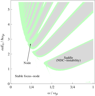
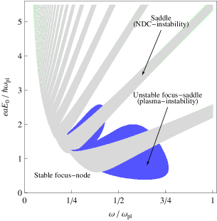
Figure 1: [Color online] Types of fixed-points of the map $G$, (a) $\omega_{\text{pl}}\tau=3$, (b) $\omega_{\text{pl}}\tau=12$. For all $\omega_{\text{pl}}\tau$ the ndc-instability is present, visible here as the regions where the fixed-point is a saddle [gray]. Equilibrium is a stable focus-node [white] for the rest of the shown parameter range, except near the borders of ndc-instability, where it is a node [green]. In (a) the ndc type is the only instability, but in (b) also the focus can destabilize, resulting in the region where the point is an unstable focus-saddle [blue].

II Plasma instability

Our focus are the instabilities occurring in the symmetric limit-cycles of Eqs. (1). By symmetry we here refer to the invariance of the equations under the transformation $\mathcal{S}$:

$$\mathcal{S}:(t,V,W,{E_{\text{sc}}})\to(t+T/2,-V,W,-{E_{\text{sc}}}).$$ (4)

A symmetric limit-cycle is then to be understood as a cycle that is invariant in $\mathcal{S}$: $(V(t+T/2),W(t+T/2),{E_{\text{sc}}}(t+T/2))=(-V(t),W(t),-{E_{\text{sc}}}(t))$. Symmetric cycles represent a basic type of dynamics that do not support effects such as spontaneous generation of dc bias. Our interest in them lies in the fact that a loss of stability in such a cycle would imply a transition to some different types of dynamics, provided no other symmetric cycles are stable for the same parameters. The stability of symmetric cycles can be studied by considering the fixed-points of the map $G$: $G(X(t))=SX(t+T/2)$, where $X(t)=(V(t),W(t),{E_{\text{sc}}}(t))$, and $S=\mathop{\mathrm{diag}}(-1,1,-1)$. Clearly, a fixed point of $G$ corresponds to a symmetric cycle of Eqs. (1). To map the parameter-space regions where a symmetric limit-cycle loses its stability, we have computed the fixed-points (equilibria) of $G$ which we then characterize according the eigenvalues of the Jacobian $J_{ij}=\partial G_{i}/\partial X_{j}$.

Our findings are shown in Fig. 1 where we have plotted the type of the equilibrium on $(\omega,E_{0})$-parameter plane for two different degrees of nonlinearity, $\omega_{\text{pl}}\tau=3$ and $\omega_{\text{pl}}\tau=12$. We have also set ${W_{\text{eq}}}=-\Delta_{0}/2$. Two types of stable equilibria are present for both cases. Typically, the equilibrium is a focus-node, implying that the steady state is reached via damped oscillations. Additionally, also node-type equilibria exist. For these, trajectories follow exponentially converging, non-oscillatory orbits onto the limiting motion.

Turning to the unstable fixed points, for plasma frequencies $\omega_{\text{pl}}\tau\lesssim 8$ the only unstable fixed-point is a saddle. These appear as the exponential convergence to a node changes to exponential divergence, and can be shown to coincide with ndc. This is shown explicitly in App. A. Since here the ndc appears at zero dc voltage, a region of absolute negative conductivity (anc) is always associated with its appearance. This leads to dynamical rectificationdunlap93:bo-f2v-conv ; ignatov95 , an effect that is studied in detail elsewherealekseev98:spont-dc ; romanov00 ; romanov01 ; isohataladc . We refer to the saddle-type instability as the ndc-instability. This instability persists for all $\omega_{\text{pl}}\tau$, and occurs approximately for $(\omega,E_{0})$ such that $eaE_{0}/(\hbar\omega)$ is a root of Bessel $J_{0}$ functionignatov95 .

As the plasma frequency is increased also the stable focus-node loses its stability, turning into an unstable focus-node in a Hopf-bifurcation. At the Hopf-bifurcation point the damped oscillations around a focus-node become diverging. This can be identified as the plasma instability of Ref. romanov79, ; *romanov79-trans as it describes just such dynamics. Importantly, the it indeed appears outside the regions of ndc, therefore suggesting that at least electric domains will not form. The lowest degree of nonlinearity that is required is $\omega_{\text{pl}}\tau\sim 8$, although values in the excess of $\sim 10$ are required to observe the effect in a reasonably large range of parameters. We note that the signature of plasma oscillations is visible for a much wider range of $\omega_{\text{pl}}\tau$ as the damped oscillations corresponding to a focus-node -type equilibrium.

In terms of superlattice parameters, the requirement of high $\omega_{\text{pl}}\tau$ can be achieved for instance for a superlattice with $n\simeq 10^{18}\;\text{cm}^{-3}$ and $\Delta_{0}\simeq 100\;\text{meV}$, with other parameters being $a=6\;\text{nm}$, $\gamma\simeq 4\;\text{THz}$ ($\tau=250$ fs). These yield $(\omega_{\text{pl}}\tau)/2\pi\simeq 8\;\text{THz}$, with values of $E_{0}\simeq 18\;\text{kV}/\text{cm}$ and $\omega/2\pi\simeq 4\;\text{THz}$ ($\hbar\omega\simeq 31\;\text{meV}$) required to reach the plasma instability region. These values are beyond what is reported in the literature for wide miniband and highly doped or low $\gamma$ superlatticesschomburg99 . On the other hand, previous theoretical studies using self-consistently calculated energy dependent scattering rates have had $\omega_{\text{pl}}\tau$ well in excess of $\leavevmode\nobreak\ 10$ near miniband centercao00:chaos-qdot-miniband . Due to field screening effects, very high $\omega_{\text{pl}}$ requires correspondingly high pump frequencies. For this reason single miniband transport model can become questionable, since it requires that $\hbar\omega\ll\Delta_{g}$, where $\Delta_{g}$ is the gap between first and second minibands.

To gain better understanding of the dynamics and physics of the instability, we transform our equations into nearly Hamiltonian variables, i.e. into a form that differs from a Hamiltonian by a small parameter. We rewrite our equations in terms of new variables $q$, $p$, and $\Delta$:

$$V=\frac{a\Delta}{2\hbar}\sin\frac{ap}{\hbar},\quad W=-\frac{\Delta}{2}\cos\frac{ap}{\hbar},$$ (5a)

$${E_{\text{sc}}}=-\frac{4\pi}{\varepsilon_{0}}eNq.$$ (5b)

Physically, $p$ is the mean value of the electron ensemble (quasi)momentum while $\Delta$ describes an effective instantaneous miniband width, reduced from $\Delta_{0}$ due to the spreading of the electron distribution in momentum space. More precisely, the fraction $\Delta/\Delta_{0}=1-\mathcal{V}$, where $\mathcal{V}$ is the variance of the momentum distribution (using a definition appropriate for periodic distribution functions). By the virtue of being the opposite of the variance, $\Delta/\Delta_{0}$ describes the coherence of the ensemble motion, i.e. the concentration (bunching) of the electrons to the vicinity of the mean momentum $p$. The interpretation of these variables is rigorously justified in Appendix B.

Substituting the above to Eqs. (1) we obtain

$$\dot{\Delta} = -\gamma\left[\Delta+2{W_{\text{eq}}}\cos\frac{ap}{\hbar}\right],$$ (6a)

$$\dot{p} = e{E_{\text{ext}}}-\frac{4\pi e^{2}N}{\varepsilon_{0}}q+2\gamma\frac{\hbar{W_{\text{eq}}}}{a\Delta}\sin\frac{ap}{\hbar},$$ (6b)

$$\dot{q} = \frac{a\Delta}{2\hbar}\sin\frac{ap}{\hbar}.$$ (6c)

The new governing equations can be thought of as effective semiclassical equations of motion for an electron ensemble. A notable difference is that $\Delta$ is here a dynamic variable rather than a constant, and that the self-consistent field, acting essentially as a harmonic returning force, is present via the variable $q$.

The Hamiltonian limit, $\gamma\to 0$, of Eq. (6) has a well-studied classical analog. Defining the phase $\theta=ap/\hbar$ one sees that $\theta$ follows the equation of a driven pendulum:

$$\ddot{\theta}+\omega_{\text{pl}}^{2}\frac{\Delta}{\Delta_{0}}\sin\theta=-\frac{eaE_{0}}{\hbar}\omega\sin\omega t.$$ (7)

Previous works have also considered the pendulum limit of the superlattice balance equationsalekseev02a ; isohatala05:sbpend . These have included damping via a term $-\gamma\dot{\theta}$ on the right-hand side to model the effect of dissipation, while supposing $\Delta=\text{constant}$. However, such a system cannot capture all the dynamics observed in the third order differential equations (6). This is because for the damped second order pendulum all phase space areas contract along the flow, making Hopf-bifurcation impossible. This implies that the interaction between the high- and low frequency parts, $(q,p)$, and $\Delta$, respectively, generates the quasiperiodic oscillations.

Using Eqs. (6) we have computed analytically approximate conditions for the appearance of the Hopf-bifurcation in the weak drive limit. We defer the details of the analysis to Appendix A. Our findings show that the Hopf-bifurcation occurs for $E_{0}>E_{\text{crit}}$, where $E_{\text{crit}}\to 0$ as $\gamma\to 0$, and for frequency

$$\Omega_{\text{R}}+\mathcal{O}(\gamma^{2})<\omega<\Omega_{\text{H}}+\mathcal{O}(\gamma^{2}),$$ (8)

where $\Omega_{\text{R}}$ is the amplitude dependent natural oscillation frequency of the system, $\Omega_{\text{H}}>\Omega_{\text{R}}$ is an upper limiting frequency for the Hopf-bifurcation, and $\mathcal{O}(\gamma^{2})$ represent terms proportional $\gamma^{2}$. Both $\Omega_{\text{R}}$ and $\Omega_{\text{H}}$ tend to $\omega_{\text{pl}}$ as $E_{0}\to 0$. The plasma instability is in other words first triggered at a small positive detuning from the resonance $\omega=\Omega_{\text{R}}$, and exists for a modest range of parameters extending to higher frequencies from resonance, and can be brought about by even a small $E_{0}$ provided that $\omega_{\text{pl}}\tau$ is large enough. The frequency of the modulation of $\Delta$ and $(p,q)$ oscillation, denoted $\Omega$, is small, vanishing at the resonance $\omega=\Omega_{\text{R}}$ and increasing as parameters varied away from it.

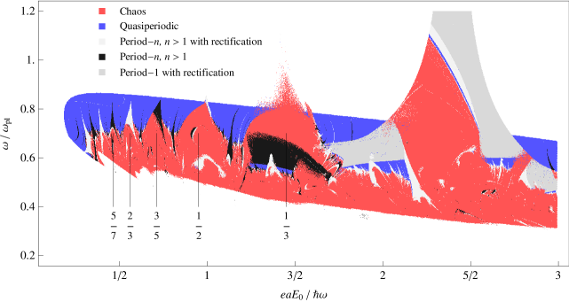
Figure 2: [Color online] Regions of different types of dynamics, $\omega_{\text{pl}}\tau=20$. Quasiperiodic motion [blue], frequency-locking [light gray and black], or chaos [red] appears as a result of the plasma instability. For tongues with locking ratios $p/q$, indicated by the labels for select resonances, such that either $p$ or $q$ is even [light gray regions] a spontaneous dc-voltage is present. Transition to chaos is associated with overlapping of the resonance tongues. The region of period-1 solutions with rectification near $eaE_{0}\sim 2.4\hbar\omega$ extending to high-frequencies outside the shown range is born out of the first ndc-instability region.

Turning to physics point of view, the analytic results show that the most significant contributing factor to the appearance of the instability is the coupling between the slow degree of freedom $\Delta$ to the resonance frequency $\Omega_{\text{R}}$, and in turn, the down mixing of the fast oscillations to the motion of $\Delta$. This is in direct analogy to what is found for coupled high- and low-frequency oscillatorsshygimaga98 , where a very feedback coupling between slow and fast parts was found to lead to a Hopf-bifurcation followed by transition to chaotic motion. Physically, $\Delta$ affects the resonance frequency via the coherence $\Delta/\Delta_{0}$. This is easily seen by noting that the resonance frequency is proportional to the frequency of free linear oscillations, $\omega_{\text{pl}}\sqrt{\Delta/\Delta_{0}}$ [cf. Eq. (7)], essentially a coherence-dressed plasma frequency. Thus, the slow motion of $\Delta$ couples to the fast oscillations by modulating the resonance frequency, and thereby affecting a change in the amplitude of the $p,q$ oscillations, with strongest response occuring near $\omega\sim\Omega_{\text{R}}$.

The reverse coupling, i.e. down mixing of fast to slow motion, is due to scattering induced loss of coherence, described by Eq. (6a). The rate of decoherence increses as the mass of the electron distribution is offset from the band bottom, since scattering events in the present model return electrons to the thermal distribution that is centered to $p=0$. Given the change in $\Delta$ is essentially adiabatic at the present range of parameters, the decoherence per drive cycle is then dependent on the amplitude of $p,q$ oscillations, with large amplitudes contributing a larger loss of coherence. This way a slow modulation of the fast oscillation amplitude is converted back to a variation in the coherence.

III Synchronization, rectification, and chaos

The Hopf-bifurcation introduces a new frequency into the system by essentially generating spontaneous oscillations that appear as a parametric self-excitation, as can be seen from Eq. (7) and noting that $\Delta/\Delta_{0}$ is now a slowly oscillating function. It is expected, then, that this generates new dynamics, and in this section we discuss the various limiting dynamics that we have found in numerical simulations of Eqs. (1).

We have observed three different types of motion as a trajectory evolves away from the unstable focus: quasiperiodic oscillations, frequency locking, and chaos. In Fig. 2 we have plotted the type of attractor corresponding to fixed initial conditions of $V(0)=0,W(0)=0,{E_{\text{sc}}}(0)=0$. In this example, trajectories ejected from the unstable focus-saddle typically converge to quasiperiodic oscillations, making the attractor a torus. This introduces a new frequency into the system that is incommensurate to the drive frequency $\omega$. We denote this frequency by $\omega_{2}$, and compute it by finding the strongest peak in Fourier transforms of ${E_{\text{sc}}}$ that is not an integer multiple of $\omega$. The frequency $\omega_{2}$ is related to the slow modulation frequency of the previous section by $\omega_{2}\simeq\omega\pm\Omega$. This relation is exact only for small plasma oscillations, and typically it is the minus sign that applies (frequency approximately $\omega+\Omega$ is present in the frequency spectrum, but is much weaker).

Of particular interest is the application of the quasiperiodic oscillations to detection of THz-radiation. To this end, spontaneous dc voltages such as those appearing at the ndc-instability would be desirable. However, the Fourier transforms of the net electric field $E$ on the tori show no zero harmonic component. The Hopf-bifurcation is super-critical and so the amplitude of the plasma oscillations is small near the bifurcations, but grows rapidly away from the critical curve. The frequency $\omega_{2}$ varies between $\omega_{\text{pl}}$ and $0$, with the frequency decreasing as the ndc-regions are approached.

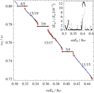
Figure 3: Main figure: Frequency of the plasma oscillations as a function of applied field amplitude $E_{0}$, $\omega_{\text{pl}}\tau=20$, $\omega\tau=14.1$. Black and gray dots correspond to stable and unstable phase-locked solutions ($\omega_{2}/\omega$ rational), respectively, while blue points mark irrational frequency ratios. Chaos [red] is seen to occur where the curve becomes dense with plateaus, e.g. near and between 7:9 and 13:17 resonances. Inset: Generated spontaneous dc-field, $\langle{E_{\text{sc}}}\rangle$ over the same range of $E_{0}$. Strong resonances at $\omega_{2}=3/4\cdot\omega$ and $\omega_{2}=4/5\cdot\omega$ are clearly visible as relatively large peaks in the dc bias.

For decreasing $\omega$ the plasma oscillation amplitude increases. This increases the coupling of $\omega$ and $\omega_{2}$ modes resulting in synchronization of the plasma oscillations to the drive. When in synchrony, the relationship

$$p\omega=q\omega_{2},$$ (9)

where $p$ and $q$ are integers, holds for a finite range of parameters. For $\omega_{\text{pl}}\tau\gtrsim 10$, the frequency locking regions appear as Arnol’d tongues in and around the quasiperiodic regime. On the tongues the period of the motion starts as $q$ times the period of the pump field $T$, and increases via period doubling bifurcations as chaotic regime is approached. A more detailed picture is provided in Fig. 3, where we have plotted $\omega_{2}/\omega$ over a range crossing multiple Arnol’d tongues. The curve bears the shape of a classic Devil’s staircase where the plateaus indicate frequency locking. Significantly, if either $q$ or $p$ is even, or if a period doubling has occurred, we observe a spontaneous generation of a weak, unquantized dc bias. In the inset of Fig. 3 we have plotted the value of dc-electric field across the superlattice, $\langle E\rangle=\langle{E_{\text{sc}}}\rangle$. Non-zero values in the dc component can be seen at even valued resonances, however, no quantization is present. The fact that no ndc is observed, implies that synchronization can be used in the detection of intense THz-radiation. We note that tongues with locking ratios such that $p,q\gg 1$ are seen only emerging inside the region of plasma instability. On the other hand, for locking ratios 1:2 and 1:3 the corresponding tongue survives outside the plasma instability regime. Although the initial conditions used in Fig. 2 prefer the period-1 solutions, these synchronization regions persist to higher $\omega$ than the quasiperiodic oscillations. This means that the 1:2 resonance can in principle be used for THz detection via ac to dc bias conversion in a wider range of parameters.

The resonance tongues form a border between quasiperiodic and chaotic oscillations. For decreasing $\omega$, the mode-locked plateaus widen and more of them appear, viz. Fig. 2. Accordingly, the staircase starts to show distinct fractal character as steps form on shorter and shorter length scales. Transition to chaos is then observed as nearby plateaus overlap. This is seen in Fig. 3 for example near 3:4 resonance and between 7:9 and 13:17 resonances. Note that the resonance plateaus are still present, but unstable and embedded in the chaotic attractor. Onset of chaos in this system can therefore be seen as following the overlapping of nearby resonanceschirikov79 , implying the collision of the heteroclinic cycles connecting the saddle points associated with the $q$-periodic orbit.

The route to chaos as observed here is a “universal” type of route to chaos also in dissipative, drive oscillatory systems jensen84 ; *bohr84; knudsen91 ; feingold88 , and dissipative systems with two competing frequencies. These include systems described by the ac+dc driven and damped pendulum equation, such as Stewart-McCumber stewrt ; *mccumber model of Josephson junctions, and systems reducing to circle maps or similar dissipative standard-like maps. A notable difference here is that the second frequency is self-generated via the Hopf-bifurcation, and not e.g. an additional external drive term.

IV Summary

We have performed an extensive study of the dynamics of the plasma instability in semiconductor superlattices under intense THz-radiation. We found an analog of the instability occurring for wide-miniband, highly doped superlattices that was studied in Ref. romanov79, ; *romanov79-trans. This instability is different from that associated with negative differential conductivity, and appears for parameters where electron transport is expected to be stable against domains.

The instability leads to sustained oscillations that are quasiperiodic at some $\omega_{2}$, frequency locked whereby $\omega_{2}$ is fixed to a rational multiple of pump-field, $\omega_{2}=(p/q)\omega$, or chaotic. Importantly from an applications point of view, the synchronization of the plasma oscillations to the drive, $p\omega=q\omega_{2}$, with an even $p$ or $q$, generates a spontaneous dc voltage that can be used in detection of THz radiation. In particular, the $p=1$, $q=2$ resonance appears particularly strong, and survives for a wide range of parameters.

Transition to chaos was found to occur as resonance tongues overlap, showing that the plasma instability is a precursor to the chaotic dynamics found in semiconductor superlattices in previous works. Indeed, it appears that this instability underlies much of the complex dynamics observed in highly-doped semiconductor superlattices. Finally, we also elucidated the physical mechanism sustaining the plasma oscillations. We found that scattering induced down-mixing of high-frequency oscillations into a slow modulation of resonance frequency of free miniband electrons is mainly responsible for the appearance of the instability.

Appendix A Details of mathematical analysis

A.1 Negative differential conductivity implies instability

Consider a symmetric limit cycle and introduce an $E$-field probe of the form ${\tilde{E}}_{\Omega}\cos(\Omega t)$ where $\Omega$ is an arbitrary probe frequency and ${\tilde{E}}$ is the probe amplitude. ${\tilde{E}}$ is assumed to be slowly varying. The probe induces a change in the current density of the form $j\to j+\partial j/\partial{\tilde{E}}_{\Omega}$. So being, we can write the time-evolution of ${\tilde{E}}$ from Eq. (1c) as

$${\dot{\tilde{E}}}_{\Omega}\cos\Omega t-\Omega{\tilde{E}}_{\Omega}\sin\Omega t=-\frac{4\pi}{\varepsilon_{0}}\frac{\partial j}{\partial{\tilde{E}}_{\Omega}}{\tilde{E}}_{\Omega}.$$ (10)

Multiplying by $\cos\Omega t$ and averaging over $T$ one obtains Eq.

$${\dot{\tilde{E}}}_{\Omega}=-\frac{4\pi}{\varepsilon_{0}}\Re\{\sigma_{\Omega}\}{\tilde{E}}_{\Omega},$$ (11)

where $\sigma_{\Omega}$ is the differential conductivity at frequency $\Omega$, $\sigma_{\Omega}=2\partial\langle j\exp(i\Omega t)\rangle/\partial{\tilde{E}}_{\Omega}$, $\Omega>0$, and $\sigma_{0}=\partial\langle j\rangle/\partial{\tilde{E}}_{0}$. The damping rate of the probe field is then $(4\pi/\varepsilon_{0})\Re\{\sigma_{\Omega}\}$, and thus, if $\sigma_{\Omega}<0$, the probe is unstable, and if $\Omega>0$, the corresponding limit-cycle is clearly a unstable focus-saddle. For $\sigma_{0}<0$ the local divergence is exponential and not oscillatory, making the unstable point a saddle.

A.2 Plasma instability

Here we present the details of the analytic formulas for the appearance of the plasma instability. For simplicity, we consider here the limit $eE_{0}\ll\hbar\omega$. We approximate $(p,q)$ with a single $\omega$ harmonic with slowly varying amplitude and phase $R,\Phi$,

$$p=\frac{\hbar R}{a}\sin(\omega t+\Phi),\quad q=\frac{\hbar\omega\varepsilon_{0}R}{4\pi e^{2}N}\cos(\omega t+\Phi).$$ (12)

We substitute these into Eqs. (6), solve for the derivatives of the new variables, and finally, apply the averaging methodverhulst05 to get the following equations for $\Delta,R$, and $\Phi$:

$$\dot{\Delta} = -\gamma(\Delta-\Delta^{*}(R)),$$ (13)

$$\dot{R} = -\Gamma R+\frac{aeE_{0}}{2\hbar}\sin\Phi,$$ (14)

$$\dot{\Phi} = -\frac{1}{2}\left(\omega-\frac{\Omega_{\text{R}}}{\omega}\right)+\frac{aeE_{0}}{2\hbar R}\cos\Phi,$$ (15)

where $J_{k}$ is the $k$th order Bessel function of the first kind, $\Delta^{*}(R)=2|{W_{\text{eq}}}|J_{0}(R)$, $\Gamma(\Delta,R)=2\gamma|{W_{\text{eq}}}|J_{1}(R)/R\Delta$, and $\Omega_{\text{R}}$ is the free, unforced, undamped oscillation frequency,

$$\Omega_{\text{R}}(R,\Delta)^{2}=\omega_{\text{pl}}^{2}\frac{\Delta}{\Delta_{0}}\frac{2J_{1}(R)}{R}.$$ (16)

Approximate symmetric limit cycles are given by steady-state values of $R,\Phi$, and $\Delta$. The phase $\Phi$ can be eliminated from the equations, while $\Delta=\Delta^{*}(R)$ and $R$ satisfies the implicit equation

$$R^{2}=\left[\frac{eaE_{0}}{\hbar}\right]^{2}\frac{1}{(2\Gamma)^{2}+\left(\omega-\frac{\Omega_{\text{R}}^{2}}{\omega}\right)^{2}}.$$ (17)

Dynamics near the equilibrium are determined by the Jacobian of the left-hand side of Eqs. (15). Frequency of small plasma oscillations is found up to first order in $\gamma$ to be

$$\Omega=\sqrt{\left(\frac{\omega}{2}-\frac{\Omega_{\text{R}}^{2}}{2\omega}\right)\left(\frac{\omega}{2}-\frac{\Omega_{\text{S}}^{2}}{2\omega}\right)}+\mathcal{O}(\gamma^{2}),$$ (18)

where the second frequency $\Omega_{\text{S}}$ arises from $R$ dependence of the $\Omega_{\text{R}}$,

$$\Omega_{\text{S}}^{2}={\tilde{\omega}}_{\text{pl}}^{2}J_{0}(R)\left[J_{0}(R)-J_{2}(R)\right],$$ (19)

where ${\tilde{\omega}}_{\text{pl}}^{2}=2|{W_{\text{eq}}}|\omega_{\text{pl}}^{2}/\Delta_{0}$. Frequencies $\Omega_{\text{R}}$ and $\Omega_{\text{S}}$ satisfy $\Omega_{\text{S}}<\Omega_{\text{R}}$ for all $\omega$ and $R$, thus, the frequency $\Omega$ is real for $\omega<\Omega_{\text{S}}$ and $\omega>\Omega_{\text{R}}$.

Instability regions are given by applying the standard Routh-Hurwitz stability criterion to the characteristic polynomial of the Jacobian:

$$\frac{1}{4}\left(\omega-\frac{\Omega_{\text{R}}}{\omega}\right)\left(\omega-\frac{\Omega_{\text{H}}}{\omega}\right)+(2\gamma-\Gamma)(\Xi+\Gamma)<0,$$ (20a)

$$\frac{1}{4}\left(\omega-\frac{\Omega_{\text{R}}}{\omega}\right)\left(\omega-\frac{\Omega_{\text{M}}}{\omega}\right)+\Gamma(\Xi-\Gamma)<0,$$ (20b)

where $\Omega_{\text{H}}>\Omega_{\text{R}}$ and $\Omega_{\text{M}}<\Omega_{\text{R}}$ are $\gamma\to 0$ upper Hopf-bifurcation limit and lower nonlinear resonance limit, respectively,

$$\Omega_{\text{H},\text{M}}^{2}=\Omega_{\text{S}}^{2}\pm 2{\tilde{\omega}}_{\text{pl}}^{2}J_{1}(R)^{2},$$ (21)

and

$$\Xi=\gamma\left[1-\frac{J_{1}(R)}{RJ_{0}(R)^{2}}(J_{0}(R)+RJ_{1}(R))\right].$$ (22)

First of the inequalities 20 is true in the presence of the plasma instability, while the second holds for the instability arising from the nonlinear resonance. In short, Eqs. (20) describe two instability bands, one below resonance (arising from multistability) and second above resonance (plasma instability). Noting that the second term in both inequalities is $\mathcal{O}(\gamma^{2})$, Eq. (8) follows.

Finally, the second term in Eq. (21), is critical for the plasma instability. If it were too small, $\Omega_{\text{H}}$ would fall below $\Omega_{\text{R}}$, and the instability would not appear. Looking in an earlier stage of the derivation, this term equals

$$\alpha=2R\Omega_{\text{R}}\frac{\partial\Delta^{*}}{\partial R}\frac{\partial\Omega_{\text{R}}}{\partial\Delta}.$$ (23)

This crucially depends on the strength of the coupling of the amplitude of the fast oscillations to $\Delta$ ($\partial\Delta^{*}/\partial R$ coefficient), and the coupling $\Delta$ to the free oscillations frequency ($\partial\Omega_{\text{R}}/\partial\Delta$ coefficient). This leads us to conclude that the down-mixing of the fast motion in the equation for $\Delta$ and the subsequent modulation of the free oscillation frequency is the main physical mechanism generating and sustaining the plasma oscillations.

Appendix B $p$ is the ensemble mean quasimomentum, $\Delta/\Delta_{0}$ coherence

Here we justify our claim that $p$ as introduced in Eqs. (5) is the center of mass of the electron distribution in (quasi)momentum space, while $\Delta/\Delta_{0}$ describes the coherence of Bloch oscillations, or the concentration (bunching) of the electrons to vicinity of the mean momentum. We will use the short-hand notations $\theta=ap/\hbar$ and $A=\Delta/\Delta_{0}$.

Let $f(p_{z},t)$ be the electron momentum distribution function as given by the Boltzmann transport equation, where $p_{z}$ is the momentum along the direction of the current, and let overline denote averaging against $f(p_{z},t)$, $\overline{(\cdot)}=(a/\pi\hbar)\int_{-\pi\hbar/a}^{\pi\hbar/a}(\cdot)f(p_{z},t)\;\mathrm{d}p_{z}$. Due to the miniband structure, $f(p_{z},t)$ is a periodic function of $p_{z}$, and for conveniance we express $p_{z}$ by an angle $\phi$, $\phi=ap_{z}/\hbar$, $-\pi<\phi\leq\pi$. We first note that the naïve expectation value of the angle $\overline{\phi}$, cannot correctly represent the center of mass position, and consequently $\overline{p}_{z}$ is not a suitable choice as the mean momentum. This becomes clear by considering $f(\phi,t)$ that is condensed to a narrow, symmetric peak at $\phi=\pi$. In such a case, the expectation value $\overline{\phi}=0$, in complete opposition to the “true” value of $\pi$.

A more appropriate definition for the mean angle, which we will denote by $\phi^{*}$, is given via the first trigonometric moment $m_{1}$ of the distributionmardia :

$$\phi^{*}=\arg m_{1},\quad m_{1}=\overline{\exp(i\phi)},$$ (24)

where $\arg z$ gives the complex argument of $z$. Furthermore, in analogy to the use of variance of distributions on the real line, the spread of a circular distribution can be characterized by its circular variance $\mathcal{V}$,

$$\mathcal{V}=1-|m_{1}|.$$ (25)

Note that $0\leq\mathcal{V}\leq 1$. Zero $\mathcal{V}$ is equivalent to the entire distribution being concentrated to the mean angle $\phi^{*}$, while unity $\mathcal{V}$ implies that a well-defined mean angle does not exist.

We show next that $\phi^{*}$ and $\mathcal{V}$ coincide with $\theta$ and $1-A$. Returning to the definition of $V$ and $W$,

$$V=V_{\text{max}}\overline{\sin(ap_{z}/\hbar)},\quad W=-\frac{\Delta_{0}}{2}\overline{\cos(ap_{z}/\hbar)}.$$ (26)

From Eqs. (5) and (26) one finds that

$$A\sin\theta=\overline{\sin(ap_{z}/\hbar)},\quad A\cos\theta=\overline{\cos(ap_{z}/\hbar)},$$ (27)

or equivalently $A\exp(i\theta)=\overline{\exp(i\phi)}$. It then follows directly from the definitions, Eqs. (24) and (25) that $\theta=\phi^{*}$ and $\mathcal{V}=1-A$. Scaling angles back to momentum units, we have $p^{*}=\hbar\phi^{*}/a=\hbar\theta/a=p$, proving our assertion that $p$ is the center of mass momentum.

References

- (1) A. Wacker, Phys. Rep. 357, 1 (2002)
- (2) K. N. Alekseev, G. P. Berman, D. K. Campbell, E. H. Cannon, and M. C. Cargo, Phys. Rev. B 54, 10625 (1996)
- (3) J. C. Cao, H. C. Liu, and X. L. Lei, Phys. Rev. B 61, 5546 (2000)
- (4) Y. A. Romanov and Y. Y. Romanova, J. Exp. Theor. Phys. 91, 1033 (2000)
- (5) K. N. Alekseev, E. H. Cannon, J. C. McKinney, F. V. Kusmartsev, and D. K. Campbell, Phys. Rev. Lett. 80, 2669 (1998)
- (6) K. N. Alekseev and F. V. Kusmartsev, Phys. Lett. A 305, 281 (2002)
- (7) K. N. Alekseev, P. Pietiläinen, J. Isohätälä, A. A. Zharov, and F. V. Kusmartsev, Europhys. Lett. 70, 292 (2005)
- (8) J. Isohätälä, K. N. Alekseev, L. T. Kurki, and P. Pietiläinen, Phys. Rev. E 71, 066206 (2005)
- (9) J. Isohätälä and K. N. Alekseev, Chaos 20, 023116 (2010)
- (10) S. A. Ktitorov, G. S. Simin, and V. Y. Sindalovskii, Fiz. Tverd. Tela 13, 2230 (1971)
- (11) S. A. Ktitorov, G. S. Simin, and V. Y. Sindalovskii, Sov. Phys. Solid State 13, 1872 (1972)
- (12) M. Büttiker and H. Thomas, Phys. Rev. Lett. 38, 78 (1977)
- (13) Y. A. Romanov, Fiz. Tverd. Tela 21, 877 (1979)
- (14) Y. A. Romanov, Sov. Phys. Solid State 21, 513 (1979)
- (15) A. A. Ignatov, E. Schomburg, J. Grenzer, K. F. Renk, and E. P. Dodin, Z. Phys. B 98, 187 (1995)
- (16) K. N. Alekseev, E. H. Cannon, J. C. McKinney, F. V. Kusmartsev, and D. K. Campbell, Physica D 113, 129 (1998)
- (17) Y. A. Romanov, J. Y. Romanova, L. G. Mourokh, and N. J. M. Horing, J. Appl. Phys. 89, 3835 (2001)
- (18) D. H. Dunlap, V. Kovanis, R. V. Duncan, and J. Simmons, Phys. Rev. B 48, 7975 (1993)
- (19) J. Isohätälä and K. N. Alekseev(2011), unpublished
- (20) E. Schomburg, M. Henini, J. M. Chamberlain, D. P. Steenson, S. Brandl, K. Hofbeck, K. F. Renk, and W. Wegscheider, Appl. Phys. Lett. 74, 2179 (1999)
- (21) D. V. Shygimaga, D. M. Vavriv, and V. V. Vinogradov, IEEE Trans. Circuits Syst. I 45, 1255 (1998)
- (22) Numerical data of Ref. \rev@citealpshygimaga98 shows traces of regions of synchronization. This phenomenon was not investigated, however, possibly because the numerical methods were not able to detect frequency locking.
- (23) B. V. Chirikov, Phys. Rep 52, 263 (1979)
- (24) M. H. Jensen, P. Bak, and T. Bohr, Phys. Rev. A 30, 1960 (1984)
- (25) T. Bohr, P. Bak, and M. H. Jensen, Phys. Rev. A 30, 1970 (1984)
- (26) C. Knudsen, J. Sturis, and J. S. Thomsen, Phys. Rev. A 44, 3503 (1991)
- (27) M. Feingold, D. L. Gonzales, O. Piro, and H. Viturro, Phys. Rev. A 37, 4060 (1988)
- (28) W. C. Stewart, Appl. Phys. Lett. 12, 277 (1968)
- (29) D. E. McCumber, J. Appl. Phys. 39, 3113 (1968)
- (30) F. Verhulst, Methods and Applications of Singular Perturbations (Springer, 2005)
- (31) K. Mardia and P. Jupp, Directional statistics, Wiley series in probability and statistics (Wiley, 2000)