Solving the accuracy-diversity dilemma via directed random walks

Abstract

Random walks have been successfully used to measure user or object similarities in collaborative filtering (CF) recommender systems, which is of high accuracy but low diversity. A key challenge of CF system is that the reliably accurate results are obtained with the help of peers’ recommendation, but the most useful individual recommendations are hard to be found among diverse niche objects. In this paper we investigate the direction effect of the random walk on user similarity measurements and find that the user similarity, calculated by directed random walks, is reverse to the initial node’s degree. Since the ratio of small-degree users to large-degree users is very large in real data sets, the large-degree users’ selections are recommended extensively by traditional CF algorithms. By tuning the user similarity direction from neighbors to the target user, we introduce a new algorithm specifically to address the challenge of diversity of CF and show how it can be used to solve the accuracy-diversity dilemma. Without relying on any context-specific information, we are able to obtain accurate and diverse recommendations, which outperforms the state-of-the-art CF methods. This work suggests that the random walk direction is an important factor to improve the personalized recommendation performance.

I Introduction

Due to the rapidly expanding internet and social network, we are overloaded by the unlimited information on the World Wide Web Faloutsos99 . For instance, one has to choose among thousands of candidate commodities to shop online, and finds the relevant information from billions of Web pages. Comprehensive exploration for each user is infeasible Broder00 . Consequently, how to efficiently help people obtain information that they truly need is a challenging task nowadays Adomavicius05 . A landmark for information filtering is the use of search engine, by which users could find the relevant web pages with the help of properly chosen keywords Brin1998 ; Kleinberg1999 . However, sometimes users’ tastes or preferences evolve with time and can not be accurately expressed by keywords, and search engines do not take into account the personalization and tend to return the same results for people with far different needs. Being an effective tool to address this problem, recommender systems have become a promising way to filter out the irrelevant information and recommend potentially interesting items to the target user by analyzing their interests and habits through their historical behaviors Adomavicius05 ; Herlocker2004 ; Konstan1997 ; Huang2004 ; Liu2009 ; Liu2008b ; Duo2009 ; Zhou2007b . Motivated by its significance in economy and society, the design of an efficient recommendation algorithm becomes a joint focus of theoretical physics Zhang2007a ; PNAS , computer science Adomavicius05 and management science Huang2004 .

Zhang et al. Zhang2007a proposed a new information framework based on the heat conduction process, namely heat-conduction-based (HC) recommendation model. HC model supposes that the objects one user has collected have the recommendation power to help the target user find potentially relevant objects. If the target user is replaced by a specific object, HC model is similar with the collaborative filtering (CF) method, in which the users rated one target object have the recommendation powers to identify the potentially interesting users. So far, CF method has been successfully applied to many online applications and has becomes one of the most successful technologies for recommender systems Liu2009 ; Liu2008b ; Duo2009 ; Zhou2007b ; PhysicaA2011 ; Pan2010 . For example, Herlocker et al. 2 proposed an algorithmic framework referring to the user similarity. Luo et al. 5 introduced the concepts of local and global user similarity based on surprisal-based vector similarity and the concept of maximum distance in graph theory. Sarwar et al. 6 proposed the item-based CF algorithm by comparing different items. Deshpande et al. 7 proposed the item-based top-$N$ CF algorithm, in which items are ranked according to the frequency of appearing in the set of similar items and the top-$N$ ranked items are returned. Gao et al. 8 incorporated the user ranking information into the computation of item similarity to improve the performance of item-based CF algorithm. Recently, some physical dynamics, including random walks Newman2006 ; Zhou2007 ; Liu2009 and the heat conduction process Zhang2007a , have found their applications in node similarity measurement. Liu et al. Liu2009 used the random walks to calculate the user similarity and found that the modified CF algorithm has remarkably higher accuracy. As a benchmark for comparison, we call it standard CF algorithm (hereinafter, CF only stands for the collaborative filtering using random-walk-based user similarity Liu2009 ). By considering the high-order correlation of the users and objects, Zhou et al. Zhou2007b and Liu et al. Liu2008b proposed the ultra accurate algorithms, in which the second-order correlations are used to delete the redundant information. Besides reliably accurate recommendations, it is also important for recommender systems to help most individuals find diverse niche objects. CF algorithms generate recommendations according to similar users’ suggestions, which prefers to rank the popular objects at the top positions of recommendation lists, leading to high accuracy but low diversity.

Random walks have been used to quantify trajectories in a symmetric ways, namely in- and out-diversity and accessibility add1 ; add2 ; add3 . In this paper, We argue that the opinions of small-degree users should be enhanced to generate diverse recommendations, and present a new directed random-walk-based CF algorithm, namely NCF algorithm, to investigate the effect of user similarity direction on recommendations. The numerical results on the data sets, Netflix and Movielens, show that the accuracy of NCF outperforms the state-of-the-art CF methods with greatly improved diversity, which suggests that the similarity direction is an important factor for user-based information filtering.

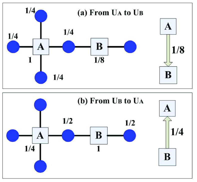
Figure 1: (Color online) Illustration of random-walk-based user similarity calculation, which has been used to measure user or object similarity in personalized recommendation. (a) The possibility walking from user $u_{A}$ to user $u_{B}$ is used to measure the directed user similarity $s_{BA}=1/8$. (b) Similarity from user $u_{B}$ to user $u_{A}$ is $s_{AB}=1/4$. The degrees of user $u_{A}$ and $u_{B}$ are $k_{u_{A}}=4$ and $k_{u_{B}}=2$, and one has $\frac{k_{u_{A}}}{k_{u_{B}}}=\frac{0.25}{0.125}$.

II Bipartite Network and heat-conduction-based model

A recommendation system consists of a set of nodes, object nodes and connections between two nodes corresponding to an object voted or collected by a user, which could be represented by a bipartite network $G(U,O,E)$. We denote the object set as $O=\{o_{1},o_{2},\dots,o_{m}\}$, the user set as $U=\{u_{1},u_{2},\dots,u_{n}\}$ and the connection set as $E=\{e_{1},e_{2},\cdots,e_{q}\}$. The bipartite network can then be represented by an adjacent matrix $A=\{a_{\alpha j}\}\in R^{m,n}$, where $a_{\alpha j}=1$ if $o_{\alpha}$ is collected by $u_{j}$, and $a_{\alpha j}=0$ otherwise.

The final aim of recommender systems is to identify a given users’ interesting objects and generate a ranking list of the target user’s uncollected objects according to the predicted scores. HC model supposes the neighbor nodes of one target node as the heat sources with temperature 1, while the remaining nodes are of temperature 0. According to the thermal equilibrium Zhang2007a , the temperature of the remaining nodes are set as the predicted scores, which could be calculated by solving the equation ${\bf W}^{h}H=\mathbf{f}$, where $\mathbf{f}$ is the flux vector Zhang2007a . The standard HC model firstly constructs the propagator matrix ${\bf W}^{h}$, where the element $w_{\alpha\beta}$ denotes the conduction rate from object $o_{\beta}$ to $o_{\alpha}$, and set the temperatures of target node’s neighbors as 1, then the heat will diffuse between heat sources and other nodes. Finally, the temperatures of uncollected objects are considered as recommendation scores.

The general framework of the item-based HC model is as follows: (i) construct the weighted object network (i.e. determine the matrix ${\bf W}$) from the known user-object relations; (ii) determine the initial resource vector $\mathbf{f}$ for each user; (iii) get the final resource distribution via

$$\mathbf{f}^{\prime}={\bf W}\mathbf{f},$$ (1)

(iv) recommend those uncollected objects with highest final scores. Note that the initial configuration $\mathbf{f}$ is determined by the user’s personal information, thus for different users, the initial configuration is different. For a given object $o_{\alpha}$, the $i$th element of $\mathbf{f}^{\alpha}$ should be zero if $a_{\alpha i}=0$. That is to say, one should not put any recommendation power (i.e. resource) onto an unrated user. The simplest case is to set a uniformly initial configuration as

$$f^{\alpha}_{i}=a_{\alpha i}.$$ (2)

Under this configuration, all the users rated object $o_{\alpha}$ have the same recommendation power.

The traditional HC model is implemented based on the object similarity. If the number of users is much smaller than the one of objects, we could apply the similar idea based on the user similarity, namely user-based HC model. From the definition, one can find that user-based HC model is equivalent to the CF algorithm, therefore, the user similarity analysis of the CF algorithm could also bring deep insight into the HC model. Zhou et al. Zhou2007 used the random walk process to calculate the node similarity of bipartite networks and proposed the network-based inference (NBI) recommendation algorithm ZhouT2008 . In Ref. PNAS , NBI algorithm was also referred as Probs algorithm. Liu et al. Liu2009 embedded the random walk process into the CF algorithm to calculate the user similarity and found that the algorithmic accuracy is greatly increased. In Ref. Liu2009 , a certain amount of resource is associated with each user, and the weight $s_{ij}$ represents the proportion of the resource $u_{j}$ would like to distribute to $u_{i}$. This process works by using the random walk process on user-object bipartite networks, where each user distributes his/her initial resource equally to all the objects he/she has collected, and then each object sends back what it has received to all the users who collect it. The weight $s_{ij}$ representing the amount of initial resource $u_{j}$ evenly transferred to $u_{i}$ can be defined as

$$s_{ij}=\frac{1}{k_{u_{j}}}\sum_{l=1}^{m}\frac{a_{li}a_{lj}}{k_{o_{l}}},$$ (3)

where $k_{u_{i}}$ and $k_{o_{l}}$ indicate the degrees of user $u_{i}$ and object $o_{l}$.

In the random walk process, the user similarity from user $u_{j}$ to $u_{i}$, $s_{ij}$, is determined by the degrees of commonly rated objects and user $u_{j}$’s degree $k_{u_{j}}$. It is unlikely these quantities are exactly the same for each pair of users, therefore, $s_{ij}\neq s_{ji}$ in most cases.

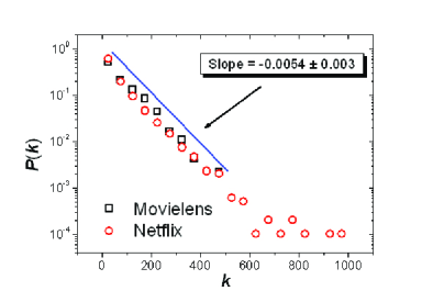
Figure 2: (Color online) User degree distributions for Movielens and Netflix data sets, which approximately have exponential forms $P(k)\sim{\rm exp}(-0.0054k\pm 0.003)$.

III Effect of User Similarity Direction on CF algorithm

According to the random-walk-based user similarity calculation (See Fig. 1), the user similarity is also calculated by random walks in a symmetric way. In CF algorithm, the system should identify the target user’s interesting objects with the help of his neighbors’ historical selections or collections. Therefore, after we obtain the user similarity matrix, the similarities from neighbors to the target user are used to evaluate the predicted scores. According to Eq. 3, to one pair of users $u_{i}$ and $u_{j}$, their similarities could be written as

$$\begin{array}[]{rcl}s_{ij}&=&\frac{1}{k_{u_{j}}}\sum_{l=1}^{m}\frac{a_{li}a_{lj}}{k_{o_{l}}},\ {{\rm From}\ u_{j}\ {\rm to}\ u_{i}};\\[10.0pt] s_{ji}&=&\frac{1}{k_{u_{i}}}\sum_{l=1}^{m}\frac{a_{li}a_{lj}}{k_{o_{l}}},\ {{\rm From}\ u_{i}\ {\rm to}\ u_{j}}.\end{array}$$ (4)

Therefore, one has

$$\frac{s_{ij}}{s_{ji}}=\frac{k_{u_{i}}}{k_{u_{j}}}.$$ (5)

If $k_{u_{i}}$$>$$k_{u_{j}}$, then $s_{ij}$$>$$s_{ji}$ and vice versa. For Movielens and Netflix data sets, the exponential forms of user degree distributions indicate that most users’ degree are very small (See Fig. 2), which means that large-degree users would frequently be identified as small-degree users’ friends. As a consequence, most users’ recommendation lists would be similar.

In order to investigate the effect of user similarity direction on CF algorithms, we introduce a new user similarity direction generated by random walks from neighbor set $U_{n}$ to the target user to measure user similarities and calculate the predicted score $v_{i\alpha}$. The NCF algorithm could be described as follows: Firstly, calculate directed user similarities according to Eq. 3, then calculate the predicted scores for target user $u_{i}$’s uncollected objects by

$$v_{i\alpha}=\frac{\sum_{j=1}^{n}s_{ij}^{\beta}a_{\alpha j}}{\sum_{ij}^{n}s_{ij}^{\beta}},$$ (6)

where $\beta$ is a tunable parameter to investigate the effect of similarity strength on the algorithmic performance, and $s_{ij}$ is the similarity from user $u_{j}$ to $u_{i}$. When $\beta=1$, all the user similarities are given the same weight; when $\beta>1$, the preferences of users with larger similarities are strengthened; when $\beta<1$, the ones with smaller similarities are strengthened. The numerical results indicate that changing the user similarity direction could not only accurately identify user’s interests, but also increase the algorithmic capability of finding niche objects.

Table 1: Basic statistics of the tested data sets.

Data Sets	Users	Objects	Links	Sparsity
MovieLens	1,574	943	82,580	$5.56\times 10^{-2}$
Netflix	10,000	6,000	701,947	$1.17\times 10^{-2}$

IV Maximal-Similarity-based CF algorithm

The algorithmic performance may be affected by the user similarity direction, and may also be determined by the properties of the data set. In other words, although the algorithmic performance of the NCF algorithm is much better than the one of the CF algorithm, it may only happen on specific data sets whose similarities from neighbors to the target user are more effective than the ones in the opposite direction. In order to make it clear, we present a maximal-similarity-based CF (MCF) algorithm to investigate the influence of similarity magnitude, in which the predicted score from user $u_{i}$ to the uncollected object $o_{\alpha}$, $v_{i\alpha}$, is given by

$$v_{i\alpha}=\frac{\sum_{j=1}^{n}s_{\rm max}^{\beta}a_{\alpha j}}{\sum_{j=1}^{n}s_{\rm max}^{\beta}},$$ (7)

where $s_{\rm max}$ is defined as the larger similarity between user $u_{i}$ and $u_{j}$

$$s_{\rm max}=\max\{s_{ij},s_{ji}\}.$$ (8)

For example, set the similarity from $u_{i}$ to $u_{j}$ is $s_{ji}=0.01$, while the one from $u_{j}$ to $u_{i}$ is $s_{ij}=0.9$. When recommending objects to $u_{i}$, the larger similarity 0.9 is used regardless of the similarity direction.

Table 2: Performances of NCF, CF and MCF algorithms for Netflix and Movielens data sets according to each of five metrics. The popularity $\langle k\rangle$, diversity $S$, precision $P$ and recall $R$ corresponding to $L=10$.

		$\langle r\rangle$	$\langle k\rangle$	$S$	$P$	$R$
	NCF	0.0450	2506	0.8236	0.0967	0.1640
Netflix	CF	0.0497	2813	0.7001	0.0917	0.1365
	MCF	0.0477	2758	0.7378	0.0954	0.1374
	NCF	0.0864	237	0.8929	0.1502	0.2037
Movielens	CF	0.1037	275	0.8435	0.1497	0.2010
	MCF	0.0970	271	0.8434	0.1459	0.1936

Table 3: Algorithmic performances for Movielens data when $p=0.9$, including the average ranking score $\langle r\rangle$, diversity $S$ and popularity $\langle k\rangle$ corresponding to length of recommendation list $L=50$. GRM is a global ranking method; CF is the collaborative filtering algorithm based on random walks Liu2009 ; Heter-CF is a modified CF algorithm, in which the user similarity is defined based on the mass diffusion process and the second-order similarity is involved ($\beta_{\rm opt}=-0.82$) Liu2008b .  CB-CF refers to the CF algorithm on weighted bipartite network PhysicaA2011 ; Hybrid is an abbreviation of the hybrid algorithm proposed in Ref. PNAS . Each number is obtained by a averaging over five ten runs with independently random division of training set and probe set.

Algorithms	Ranking score	Popularity	Hamming Distance
GRM	0.1390	259	0.398
CF	0.1063	229	0.750
Heter-CF	0.0877	175	0.826
CB-CF	0.0914	148	0.763
Hybrid	0.0850	167	0.821
NCF	0.0864	178	0.801

V Simulation Results

V.1 Data Description

In this paper, we base our simulation results on two data sets. The Movielens data set consists of 100,000 ratings from 943 users on 1,574 movies(objects) and rating scale from 1 (i.e., worst) to 5 (i.e., best). The Netflix data set add5 is a random sample of the whole records of user activities in Netflix.com, which consists of 6,000 movies and 10,000 users and 824,802 ratings. The users of Netflix also vote movies by discrete ratings from one to five. Here we apply a coarse graining method: a movie is considered to be collected by a user only if the rating is larger than 2. In this way, the Movielens data has 82,580 edges, and the Netflix data has 701,947 edges (See Table I for basic statistics). As an online movie recommendation web site, Movielens invites users to rate movies and, in return, makes personalized recommendations and predictions for movies the user has not already rated, under-contribution is common. Unlike Netflix web site, MovieLens does not have any DVD rental service. The data set $E$ is randomly divided into two parts $E=E^{T}\cup E^{P}$, where the training set $E^{T}$ is treated as known information, containing $p$ percent of the data, and the remaining $1-p$ part is set as the probe set $E^{P}$, whose information is not allowed to be used for prediction.

V.2 Metrics

V.2.1 Average ranking score

Accuracy is one of the most important metric to evaluate the recommendation algorithmic performance. An accurate method will put preferable objects in higher places. Here we use average ranking score Zhou2007 to measure the accuracy of the algorithm. For an arbitrary user $u_{i}$, if the object $o_{\alpha}$ is not collected by user $u_{i}$, while the entry $u_{i}$-$o_{\alpha}$ is in the probe set, we use the rank of $o_{\alpha}$ in the recommendation list to evaluate accuracy. For example, if there are 8 uncollected objects for user $u_{i}$, and object $o_{\alpha}$ is ordered at the 3rd place, we say the position of $o_{\alpha}$ is 3/8, denoted by $r_{i\alpha}=0.375$. Since the probe entries are actually collected by users, a good algorithm is expected to give high recommendations to them, leading to a small $r_{i\alpha}$. Therefore, the mean value of the positions, averaged over all the entries in the probe set, can be used to evaluate the algorithmic accuracy.

$$\langle r\rangle=\frac{1}{n}\sum_{i=1}^{n}\Big{(}\frac{\sum_{(u_{i},o_{\alpha})\in E^{p}}r_{i\alpha}}{q-k_{u_{i}}}\Big{)},$$ (9)

where $E^{p}$ is the edge set existing in the probe set and $q$ is the number of objects in the probe set. The smaller the average ranking score, the higher the algorithmic accuracy, and vice verse.

V.2.2 Precision and Recall

Since users usually only consider the top part of the recommendation list, a more practical metric is to consider the number of users’ hidden links ranked in the top-$L$ places. We adopt another accuracy measure called precision. For a target user, the precision is defined as the ratio between relevant objects (namely the objects collected by $u_{i}$ in the probe set) and the length $L$. Averaging the individual precisions over all users, we obtain the mean value $P(L)$ of the algorithm on one data set,

$$P(L)=\frac{1}{n}\sum_{i}\frac{d_{i}(L)}{L},$$ (10)

where $d_{i}(L)$ indicates the number of relevant objects existing in the top-$L$ places of the recommendation list. A larger precision corresponds to a better performance. Recall is defined as the ratio between the number of objects existing in the top-$L$ places of the recommendation list and the total number of collected objects $C_{i}$ in the probe set. Averaging over the individual recalls, we obtain the mean recall $R(L)$, which could be defined as

$$R(L)=\frac{1}{n}\sum_{i}\frac{d_{i}(L)}{C_{i}}.$$ (11)

The larger recall corresponds to the better performance.

V.2.3 Diversity

The analysis results on Facebook data set showed that, besides the common interests, users of online social networks also have their specific tastes and interests JPPNAS , leading to diverse selection behaviors. Liu et al. PRE2011 found that users’ tastes on Movielens and Netflix data could also be divided into two categories: common interests and specific interests. Therefore, besides accuracy, the diversity of all recommendation lists is taken into account to evaluate the algorithmic performance. In general, most of the users would not show negative altitude to popular objects, therefore, ranking popular objects at the top part of recommendation lists would generate higher accuracy. However, personalized recommendation algorithms should not only present accurate prediction but also generate different recommendations to different users according to their specific tastes or habits. The diversity can be quantified by the average Hamming distance,

$$S=1-\langle Q_{ij}(L)\rangle/L,$$ (12)

where $L$ is the length of the recommendation list and $Q_{ij}$ is the number of overlapped objects in $u_{i}$’s and $u_{j}$’s recommendation lists. The largest $S=1$ indicates recommendations to all users are completely different, in other words, the system has the highest diversity. While the smallest $S=0$ means all of recommendations are exactly the same.

V.2.4 Popularity

An accurate and diverse recommender system is expected to help users find the niche or unpopular objects which are hard for them to identify. The metric popularity is introduced to quantify the capacity of an algorithm to generate unexpected recommendation lists, which are defined as the average collected times over all recommended objects

$$\langle k\rangle=\frac{1}{n}\sum_{i}\Big{(}\frac{1}{L}\sum_{o_{\alpha}\in O^{L}_{i}}k_{o_{\alpha}}\Big{)},$$ (13)

where $O^{L}_{i}$ is $u_{i}$’s recommendation list with length $L$. A smaller average degree $\langle k\rangle$, corresponding to less popular objects, are preferred since those lower-degree objects are hard to be found by users themselves.

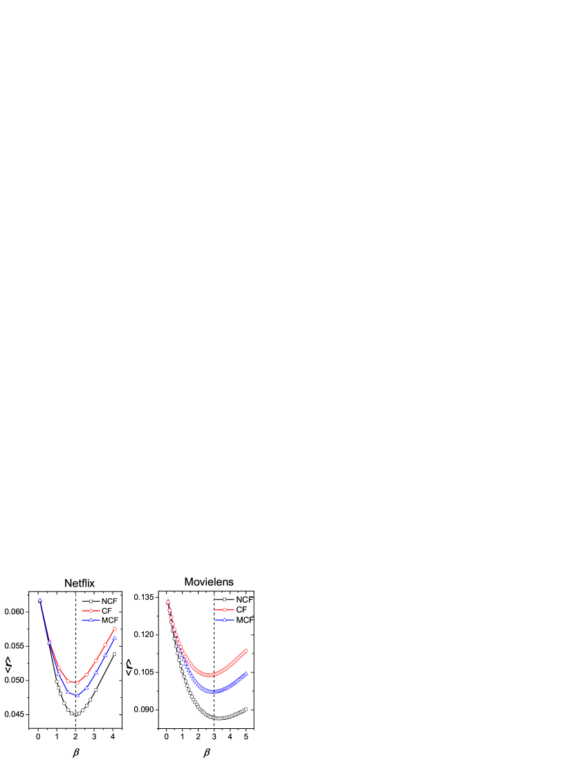
Figure 3: (Color Online) The average ranking score $\langle r\rangle$ vs. $\beta$ for NCF, CF and MCF algorithms. The optimal $\beta_{\rm opt}$ of NCF for Movielens data set, corresponding to the minimal $\langle r\rangle=0.086$, is $\beta_{\rm opt}=3.3$, the one for Netflix data set is $\beta_{\rm opt}=2.0$ corresponding to $\langle r\rangle=0.0450$. When $\beta=1$, the algorithm degenerates to the accuracy of the CF algorithm based on the new user similarity direction. All the data points are averaged over ten independent runs with different data-set divisions.

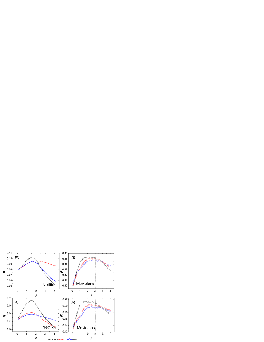
Figure 4: (Color online) Performances of the NCF, CF and MCF algorithms for MovieLens and Netflix data sets when recommendation lists equal to $L=10$. (a)-(d) show average object degrees $\langle k\rangle$ vs. $\beta$ and diversity $S$ vs. $\beta$. At the optimal cases, both popularity $\langle k\rangle$ and diversity $S$ of NCF are much better than the ones of CF and MCF algorithms. (e)-(h) Precision $P$ and recall $R$ vs. $\beta$ for Netflix and Movielens data sets. One can find that both of $P$ and $R$ of NCF for Movielens are larger than the ones of CF and MCF algorithms, while the precision $P$ for Netflix is close to the one of CF algorithm and the recall $R$ is much better than the results of CF algorithm. All the data points are averaged over ten independent runs with different divisions of training-probe sets.

V.3 Simulation Results

We summarize the results for NCF, CF and MCF algorithms, as well as the metrics for Movielens and Netflix data sets in Table II. Clearly, NCF outperforms the classical CF and MCF algorithms over all five metrics, including average ranking score $\langle r\rangle$, diversity $S$, popularity $\langle k\rangle$, precision $P$ and recall $R$. Table III gives the comparisons among different algorithms for $p=0.9$. The so-called optimal parameters are subject to the lowest average ranking score $\langle r\rangle$. The metrics, including average ranking score $\langle r\rangle$, diversity $S$ and popularity $\langle k\rangle$, are obtained at the optimal parameters. From which one can see that the accuracy of NCF is close to the result of hybrid algorithm PNAS and outperforms the state-of-the-art CF algorithms using the second-order correlation information Liu2008b . Among all algorithms, Heter-CF algorithm gives the highest diversity, while CB-CF algorithm generates the lowest popularity. Comparing with these two outstanding algorithms, NCF can reach or closely approach the best diversity without taking into account high-order correlation, and provide more accurate recommendation results.

Figure 3 reports the algorithmic accuracy as a function of $\beta$. In our algorithm, the curve (the red circle) has a clear minimum around $\beta_{\rm opt}=3.3$ for Movielens and $\beta_{\rm opt}=2.0$ for Netflix. Comparing with CF algorithms whose user similarities are defined from large-degree to small-degree users, the average ranking score $\langle r\rangle$ of NCF is reduced from 0.497 to 0.045 for Netflix and from 0.1037 to 0.0864 for Movielens data set, reduced by 9.9% and 16.68% respectively at the optimal values. Comparing with the MCF algorithm, the performance of NCF is also better. Subject to the accuracy, the reason why NCF outperforms CF and MCF indeed lies in the direction effect but not the data effect, and the results also indicate that giving more recommendation power to the small-degree users could enhance the accuracy and diversity simultaneously.

The Hamming distance $S$ is introduced to measure the algorithmic performance to present personalized recommendation lists. The average object degree $\langle k\rangle$ is used to evaluate the ability that an algorithm gives a novel recommendation. Figure 4 (a)-(d) show $\langle k\rangle$ and $S$ as a function of $\beta$ when recommendation list length $L=10$ respectively. For the Movielens data set, at the optimal point $\beta_{\rm opt}=3.3$, the popularity $\langle k\rangle=237$, which is reduced by 13.8%, and the diversity $S=0.8929$ is improved by 5.9% comparing with the ones of CF at its optimal value. When the list length $L=10$, the popularity $\langle k\rangle$ and diversity $S$ of NCF are reduced by 10.9% and 17.64% for Netflix data set. From which one can find that the NCF algorithm using the new directed random walks has the capability to find the niche objects, leading to diverse recommendations.

In general, NCF outperforms CF as well as MCF in terms of the accuracy $\langle r\rangle$, diversity $S$ and popularity $\langle k\rangle$. However, in reality, users only care about the top part of the recommendation list. From Fig. 4 (e)-(h), one can find that, comparing with the results of CF and MCF algorithms, the precision $P$ and recall $R$ of NCF are also very good. When $L=10$ with the optimal parameter corresponding to the lowest ranking score, the precision $P$ is approximately improved 3.0% and 5.5%, and the recall $R$ is roughly enhanced by 5.2% and 20.15% for Movielens and Netflix data sets respectively.

Since the similarities generated by the random walk process from small-degree to large-degree users are larger than the ones from the opposite direction, the simulation results indicate that enhancing the small-degree users’ recommendation powers increases the prediction accuracy, and helps users find niche objects, leading to more diverse recommendations. Figure 5 investigates the correlation between the target user degree $k_{u}$ and its neighbors’ average degree $\langle k_{u}^{n}\rangle$ as well as deviation $D(k_{u})$, where the target user’s neighbors $U_{n}$ are defined as the users who have at least one common rated object with the target user, which could be obtained from the adjacent matrix $A$. Denoting the user correlation matrix as $C^{\rm user}$, we have $C^{\rm user}=AA^{T}$. The element $C^{\rm user}_{ij}$ means the number of common rated objects between user $u_{i}$ and $u_{j}$. Given a matrix $T=\{t_{ij}\}\in R^{n,n}$, with $t_{ij}=1$ if $C^{\rm user}_{ij}>0$, and $t_{ij}=0$ if $C^{\rm user}_{ij}=0$. The number of correlated neighbors $k^{c}_{u}$ for a target user $u$ could be given as $k^{c}_{u}=\sum_{j=1}^{n}t_{uj}$, then average degree $\langle k_{u}^{n}\rangle$ of correlated neighbors $U_{n}$ is defined by

$$\langle k_{u}^{n}\rangle=\frac{1}{k^{c}_{u}}\sum_{j=1}^{n}t_{uj}k_{j}.$$ (14)

The deviation $D(k_{u})$ could be given as

$$D(k_{u})=\sqrt{\frac{1}{k^{c}_{u}}\sum_{j=1}^{n}\Big{(}t_{uj}k_{j}-\langle k_{u}^{n}\rangle\Big{)}^{2}}.$$ (15)

Figure 5 shows that when $k_{u}$ is very small, both neighbors’ average degree $\langle k_{u}^{n}\rangle$ and deviation $D(k_{u})$ are very large, which means that for Movielens and Netflix data sets, the small-degree users would like to commonly rate objects with small-degree users and large-degree users. As $k_{u}$ increases, both $\langle k_{u}^{n}\rangle$ and $D(k_{u})$ would decrease correspondingly, which means that the large-degree users only commonly rate objects with small-degree users. According to our previous analysis, if the user similarities from neighbors to the target user are enhanced, the effects of the small-degree users would be emphasized to match both large-degree and small-degree users’ common and specific interests, which is the reason why directed random-walk-based user similarity is effective.

Figure 5: (a)-(b) The average degree of the target user’s neighbors $\langle k_{u}^{n}\rangle$ and the corresponding deviation $D(k_{u})$ vs. target user degree $k_{u}$ for Netflix data set. (c)-(d) show the results for Movielens. To small-degree users, both their neighbors’ average degree $\langle k_{u}^{n}\rangle$ and the deviation $D$ are very large. As $k_{u}$ increases, $\langle k_{u}^{n}\rangle$ and $D(k_{u})$ would decease correspondingly.

VI Effects of data sparsity

We investigate the effects of the data sparsity on the performance. Since we focus on the similarity direction effect on the CF algorithm, we choose the classical CF algorithm for comparison. In the simulation work, we select $pE$ edges as training set, and set the rest $(1-p)E$ edges as probe set. Lower $p$ means less information is used to generate the recommendations. The numerical results for Movielens are shown in Fig. 6. Each point of the histogram is obtained with the optimal parameter subject to the lower ranking score. The improvement function $f(\langle r\rangle)$ of the present algorithm is defined as

$$f(\langle r\rangle)=\frac{\langle r\rangle_{\rm CF}-\langle r\rangle_{\rm NCF}}{\langle r\rangle_{\rm CF}}.$$ (16)

For the popularity $\langle k\rangle$ and Hamming distance $S$, the improvement functions are defined as

$$\begin{array}[]{c}f(\langle k\rangle)=\frac{\langle k\rangle_{\rm CF}-\langle k\rangle_{\rm NCF}}{\langle k\rangle_{\rm CF}},\\[12.0pt] f(S)=\frac{S_{\rm NCF}-S_{\rm CF}}{S_{\rm CF}}.\end{array}$$ (17)

Figure 6 shows that the improvement of average ranking score $\langle r\rangle$ decreases as the size of the training set decreases, which may be come from the fact that the number of neighbors would decrease and less information could be used to predict the target user’s interests. We also found NCF performs much better than CF for denser datasets. The improvement of diversity $f(S)$ decreases with the increasing size of training set, and $f(\langle k\rangle)$ increases with more denser training set, which indicate that, generally speaking, users prefer to select popular objects as they give more ratings.

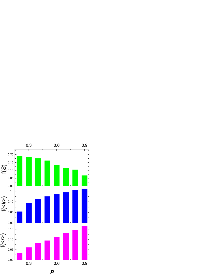
Figure 6: Improvements of the average ranking score $\langle r\rangle$, average objects degree $\langle k\rangle$ and diversity $S$ to different sparsity of the training set for Movielens data set. All the data points are averaged over ten independent runs with different data set divisions.

VII Conclusion and Discussions

In this paper, by tuning the random walk direction from neighbors to the target user to calculate the directed user similarity, we investigate the physics of directed random walks and their influence on the information filtering of user-object bipartite networks. Simulation results indicate that the new CF algorithm using the new directed random walks outperforms state-of-the-art CF methods in terms of the accuracy, as well as the Heter-CF algorithm in terms of diversity simultaneously. Meanwhile NCF has much better capability to present more accurate and diverse recommendations than CF algorithms whose user similarities are calculated from the target user to neighbors. The accuracies of NCF algorithms are close to the results of the hybrid algorithm PNAS , and the diversities are also increased dramatically.

CF algorithms are one of the most successful information filtering algorithm and has been extensively used on lots of web sites, such as Netflix and Amazon. HC model also has been successfully used for information filtering. If we suppose the users rated one specific objects are the heat source, CF algorithms are equivalent to the user-based HC model. Although random walks have been used to improve the user or object similarity measurement PNAS ; Liu2009 , the reason why directed similarity could enhance the information filtering performance is missing. Since the idea of the CF algorithm is combing neighbors’ opinions of the target user to predict his interests or habits, we always suppose that the CF algorithm would like to converge users’ interests and present popular objects. But the analysis in this paper indicates that if small-degree users’ recommendation powers are increased CF algorithm also could solve the accuracy-diversity dilemma. In most of the online social systems, the number of small-degree users is always much larger than large-degree ones. According to the random-walk-based user similarity definition, we know that similarities from small-degree users are always larger than the reversed ones. Therefore, in the CF algorithm, the opinions of the large-degree users would be recommended to most of small-degree users, leading to lower diversity. By tuning the similarities from neighbors to the target user, we could emphasize the recommendation powers of small-degree users and enhance the accuracy and diversity simultaneously, which indicates that the similarity direction is an important factor for information filtering. Although the idea of this paper is simple, the remarkable simulation results indicate that, to generate accurate and diverse recommendations, we only need to change the direction without changing the framework of the existing CF systems.

The directed random walk process presented in this paper indeed has been defined as a local index of similarity in link prediction Lv2 ; EPJB2009 , community detection Liu2010P and so on. Meanwhile, a number of similarities, based on the global structural information, have been used for information filtering, such as the transferring similarity Duo2009 and the PageRank index Brin1998 , communicability add4 and so on. Although the calculation of such measures is of high complexity, it’s very important to the effects of directed random walks on these measures. The hybrid algorithm PNAS is also a kind of item-based CF algorithm where the item similarity is measured by combining the random walk and heat conduction processes together. Lü et al. Linyuan2011 proposed an improved hybrid algorithm by embedding the preferential diffusion process into hybrid algorithm. Qiu et al. zike2011 proposed an improved method by introducing an item-oriented function to solve the cold-start problem. In this paper, we find that the direction of random walks is very important for information filtering, which may be helpful for deeply understanding of the applicability of directed similarity.

We thank Dr Chi Ho Yeung for his helpful suggestions. We acknowledge GroupLens Research Group for providing us MovieLens data and the Netflix Inc. for Netflix data. This work is partially supported by NSFC (10905052, 70901010, 71071098 and 71171136), JGL is supported by the European Commission FP7 Future and Emerging Technologies Open Scheme Project ICTeCollective (238597), the Shanghai Leading Discipline Project (S30501) and Shanghai Rising-Star Program (11QA1404500).

References

- (1) M. Faloutsos, P. Faloutsos and C. Faloutsos, Comput. Commun. Rev. 29, 251 (1999).
- (2) A. Broder, R. Kumar, F. Moghoul, P. Raghavan, S. Rajagopalan, R. Stata, A. Tomkins and J. Wiener, Comput. Netw. 33, 309 (2000).
- (3) G. Adomavicius and A. Tuzhilin, IEEE Trans. Knowl. Data Eng. 17, 734 (2005).
- (4) S. Brin and L. Page, Comput. Netw. ISDN Syst. 30, 107 (1998).
- (5) J. Kleinberg, J. ACM 46, 604 (1999).
- (6) J. L. Herlocker, J. A. Konstan, K. Terveen and J. T. Riedl, ACM Trans. Inform. Syst. 22, 5 (2004).
- (7) J. A. Konstan, B. N. Miller, D. Maltz, J. L. Herlocker, L. R. Gordon and J. Riedl, Commun. ACM 40, 77 (1997).
- (8) Z. Huang, H. Chen and D. Zeng, ACM Trans. Inform. Syst. 22, 116 (2004).
- (9) T. Zhou, R.-Q. Su, R.-R. Liu, L.-L. Jiang, B.-H. Wang and Y.-C. Zhang, New J. Phys. 11, 123008 (2009).
- (10) J.-G. Liu, B.-H. Wang and Q. Guo, Int. J. Mod. Phys. C 20, 285 (2009).
- (11) J.-G. Liu, T. Zhou, H.-A. Che, B.-H. Wang and Y.-C. Zhang, Physica A 389, 881 (2010).
- (12) D. Sun, T. Zhou, J.-G. Liu, R.-R. Liu, C.-X. Jia and B.-H. Wang, Phys. Rev. E 80, 017101 (2009).
- (13) Y.-C. Zhang, M. Blattner and Y.-K. Yu, Phys. Rev. Lett. 99, 154301 (2007).
- (14) T. Zhou, Z. Kuscsik, J.-G. Liu, M. Medo, J. R. Wakeling and Y.-C. Zhang, Proc. Natl. Acad. Sci. U.S.A. 107, 4511 (2010).
- (15) J.-G. Liu, Q. Guo and Y.-C. Zhang, Physica A 390, 2414 (2011).
- (16) X. Pan, G.-S Deng and J.-G. Liu, Chin. Phys. Lett. 27, 068903 (2010).
- (17) J.L. Herlocker, J.A. Konstan, A. Borchers and J. Riedl, In Proc. of SIGIR ’99, 1999, pp. 230.
- (18) H. Luo, C. Niu, R. Shen and C. Ullrich, Machine Learning 72, 231 (2008).
- (19) B. Sarwar, G. Karypis, J. Konstan and J. Riedl, In Proc. of ACM on WWW conference 2001, pp. 285.
- (20) M. Deshpande and G. Karypis, ACM Tran. Info. Syst. 22, 143 (2004).
- (21) M. Gao, Z.F. Wu, F. Jiang, Info. Proc. Lett. 111, 440 (2011).
- (22) E.A. Leicht, P. Holme and M.E.J. Newman, Phys. Rev. E 73, 026120 (2006).
- (23) T. Zhou, J. Ren, M. Medo and Y.-C. Zhang, Phys. Rev. E 76, 046115 (2007).
- (24) B. Travencolo and L. da F. Costa, Phys. Lett. A 373, 89 (2008).
- (25) B.A.N. Travenolo, M.P. Viana and L. da F. Costa, New J. of Phys. 11, 063019 (2009).
- (26) M. P. Viana, J. B. Batista and L. da F. Costa, Arxiv.org/1101.5379.
- (27) T. Zhou, L. L. Jiang, R. Q. Su and Y.-C. Zhang, Europhys. Lett. 81, 58004 (2008)
- (28) M.B. Díaz, M.A. Porter and J.-P. Onnela, Chaos 20, 043101 (2010).
- (29) J.P. Onnela and F. Reed-Tsochas, Proc. Natl. Acad. Sci. U.S.A. 107, 18375 (2010).
- (30) J.-G. Liu, T. Zhou and Q. Guo, Phys. Rev.E 84, 037101 (2011).
- (31) L. Lü and T. Zhou, Europhys. Lett. 89, 18001 (2010).
- (32) T. Zhou, L. Lü and Y.-C. Zhang, Euro. phys. J. B, 71, 623, (2009).
- (33) Y. Pan, D.-H. Li, J.-G. Liu and J.-Z. Liang, Physica A 389, 2849 (2010).
- (34) E. Estrada and N. Hatano, Phys. Rev. E 77, 036111 (2008).
- (35) L. Lü and W. Liu, Phys. Rev. E 83, 066119 (2011).
- (36) T. Qiu, G. Chen, Z.-K. Zhang and T. Zhou, EPL 95, 58003 (2011).