Orbital stability and the quantum atomic spectrum from Stochastic Electrodynamics

Abstract

(slight revision, soon some numerical estimations)

High order terms in the electromagnetic multi-pole development expose a stabilizing mechanism for the atomic orbitals in the presence of a random background of electromagnetic fluctuations. Boyer and Puthoff set forward the idea that for the Bohr orbits in the hydrogen atom, radiation losses could be compensated by absorption from the QED-predicted Zero-Point Field (ZPF) background. This balance is, on average over the orbit, a necessary condition for stationarity of the orbits, imposing a relation on the pair $R_{0}$ (orbital radius), $\omega_{0}$ (orbital angular velocity); such relation is simply what we have for long known as angular momentum (AM) quantization ($l=1$). Nothing has been said yet, however, on how could this balance be attained on a quasi instantaneous basis, in other words, how could the orbit accommodate the instantaneous excess or defect of energy so as to keep constant the (at least average) values of its parameters ($R_{0}$, $\omega_{0}$). Using classical electromagnetism, we explore some high order interactions between realistic particles, exposing a mechanism (a feedback loop between variables) that makes that stability possible. Puthoff’s work led necessarily to the quantization of AM: “if stable orbits exist… then their AM must be quantized”; now we are able to do a much stronger statement: “the equations of the system, in the presence of ZPF background, lead necessarily to a discrete set of stable orbits”.

The job is done in two steps. First, we work with an ideal electromechanical model composed of two (charged) particles: one is a point-like magnetic source and the other one consists of a spatially “extended” charge distribution, orbiting around the point like one. In the second place, a relocation of the inertial reference system and other minor changes are done to reinterpret the former picture in terms of a realistic hydrogen atom, the two situations turning out to be formally identical, but for some factor of proportionality. As a novelty in the subject, here it is the inner structure of the nucleus (and not of the electron) that plays the crucial role in our model. The following step regards the existence (for each $l$) of an infinite and discrete spectrum: the presence of a secondary feedback loop in the equations is crucial for the feasibility of excited states. Up to the order of our equations and under some further approximations, our model admits a continuum of stationary trajectories described by four parameters: $\{R_{0},\omega_{0},R_{1},\omega_{1}\}$; the first pair $(R_{0},\omega_{0})$ corresponding to the orbital movement, the latter $(R_{1},\omega_{1})$ to what we have called a “secondary oscillation” (may there from here a connection to Cavalleri and others’ model of spin as a residual helical oscillation of a point-like electron Cavalleri10 ?). Stationarity determines, for a given $R_{0}$, both $\omega_{0}$ and $\omega_{1}$ (imaginary poles in the linearized frequency description of the system), while $R_{1}$ remains free, allowing, once radiation/absorption (rad/abs) processes are considered, the power balance that is necessary for stability, while discreteness of the spectrum is now retained via an additional condition, a phase relation $\omega_{1}=n/\omega_{0}$ ($n$ integer) that we regard also necessary for stability. Such phase relation also allows us to arrive to an E-spectrum that could be made to resemble, under some approximations, the well known $1/n^{2}$ one. Of course stationarity is so far only a necessary condition for stability: more as an intermediate step than a rigorous proof, we introduce a stochastic description of the rad/abs processes, in a way that makes (at least) possible the negativity of the real part of the eigenvalues (poles in the frequency domain) of the linearized description of the system.

Obviously, circular trajectories can only give rise to $p$-orbitals (or at least $l>1$ ones): an additional (infinite and discrete) set of trajectories with no net AM can also be found, that would account for the $s$-spectrum. Both in the $s$ or $p$ cases, an atomic transition implies an emission/absorption of a wave-packet with energy $\hbar(\omega_{i}-\omega_{j})$, $\omega_{i},\omega_{j}$ being the (main) frequencies of the oscillation (primary osc.) of the orbitals involved. Besides, for the feasibility of our model, we are led to think in fully relativistic orbitals, “nodes” absent at least for $l>0$ Szabo69 ; anyway, the unrealistic nature of pure states would also solve this problem, even for $l=0$ (Fritsche). Finally, the action of the stochastic background on the oversimplified, entirely deterministic orbits that we provide here would produce a probability distribution extended to the whole space, an estimation which is left for elsewhere. We also barely touch other issues like the extension of the results to 3D, as well as to $l>1$ orbits; a preliminary exploration is, in any case, the ultimate goal of this paper.

I Prologue

The aim of this paper is to show that an elementary mechanism exists, in the context of SED (classical electromagnetism plus a zero-point background of radiation), that can be a possible explanation for the discrete and stable character of the hydrogen orbital spectrum, and by extension the atomic one in general. Such a stabilizing mechanism arises in a higher order description of the system, where an elementary model of the nucleus with some inner structure is included. When complexity is present in the structure of a systems, it is not a rare thing that its dynamics presents some stability and/or attraction phenomena, and very often far beyond the obvious. A basic analysis of orders of magnitude will be added soon; so far it does not seem to invalidate my ideas here.

I.1 Some foundations

We will be dealing here, exclusively, with classical Maxwellian electromagnetism. We have charges (or distributions of them) and fields, amongst them a random background: fluctuations of the value of the fields in the vacuum. The following ideas are both a point of departure and arrival:

(I) To be able to relate the concepts of quantum and classical angular momentum (AM), we will assume that each projection of quantum (orbital) AM corresponds to an average on (the projection of) the standard classical AM along a closed, periodic trajectory. This is justified in Sec. XVI.1: it seems almost obvious given the corresponding addition rules in QM.

(II) I assume (I) also applies to the inner AM or spin of a particle. I will often talk of a “classical spin” when referring to a rotational movement of a particle (or a distribution of particles) around an axis of symmetry. Whether if quantum spin appears in a representation where an isomorphism can be established (or not) to the group $SO(3)$ of rotations in ordinary space is a question that we have analyzed somewhere else DR_Spin ; here we are only interested in the fact that, whenever a particle has spin, at least some sort of classical AM can be associated to it (and in particular in regard to its magnitude). Besides, we are also aware there are some relativistic difficulties with the picture of a classically spinning sphere of charge and include some comments on that.

(III) Accordingly, I interpret QM as a “semi-static” theory that masks a richer dynamics underneath, involving perhaps a higher number of (hidden) classical degrees of freedom (that “complexity”): for instance, the quark dynamics (as point-like entities carrying charge and spin, but configuring a distribution, with an associated dynamics, in space) inside a nucleon.

(IV) In coherence with (III), while average values of the projections of those classical AM will stay attached to a discrete spectrum as in QM, their instantaneous values (and in a micro-dynamics that is transparent to atomic transitions) can, at least, oscillate around the quantum mechanical one. Interaction with a random background could cause much of those fluctuations, and, incidentally, spontaneous state transitions that are nothing new in orthodox QM. For instance the orbital AM of the quarks inside a proton (therefore adding to the particle’s inner AM or spin) can oscillate around its quantum value, in response to perturbations coming from the interaction with the background. Because those oscillations are more or less minimal, we propose the term “residual spin” (RS). The reference to the quark model is necessary (is solves some difficulties of the model with special relativity), but nevertheless nothing more than tangential.

(V) The concept of a “photon” ($E=\hbar\omega$) could be perhaos be understood as the natural constraint on the spectrum of these possible “discrete” exchanges of energy-momentum between metastable states of a system of charges.

I.2 An overview of results and some general context

We provide a very brief summary of the paper. Basically, what we do is: we begin this effort by analyzing an elementary electromechanical model. Later, we make the necessary changes to apply our results to an elementary model of a hydrogen atom.

Under the action of an ideal magnetic dipole, a moving charge with some spatial extension (non-vanishing second order moment) experiences a force and a torque, mediating between its “orbital” and “self rotation” degrees of freedom, this last what we will call a (classical) “residual spin” (RS). That pair (force, torque) introduces a bidirectional coupling between the (instantaneous) values of two classical angular momenta corresponding to those two degrees of freedom, a coupling that acts on their magnitude, as a difference, for instance, with the spin-orbit (LS) coupling in atomic physics, which acts only on their relative orientations: this is no surprise but only a consequence of the fact that our mechanism corresponds to terms of a higher order in the multipole development. For instance, too, the LS coupling only involves a punctual value of the field, therefore being unable to feel its gradient, which is another fundamental difference with the interaction we expose here. As we said before, we have named it, provisionally and for the lack of a better choice, Inverse Magnitude Spin Orbit coupling (IMSO).

An interpretation of our model in terms of the hydrogen atom is more elaborate, but we conclude that similar results could be applicable to the orbitals of the electron around the nucleus, when a spatially “extended” charge distribution is associated to this last, and always in the presence of a background. On the other hand, later, to be able to interpret our result in a more realistic situation (an atomic model), the role played here by that classical spin will be taken by what we have called residual spin (RS) of the nucleus: in the simplest case of a proton, a residual (inner) AM coming from orbital movement of quarks inside its structure. In the presence of a certain background compensating on average the radiative losses, we are already able to prove that the identified “feedback loop” (FL) between orbit and the RS-N provides a necessary and sufficient condition for the existence of stable “orbitals” in the classical configuration space of the system. These orbitals are produced by oscillations around a set of privileged trajectories or “attractors”, that (we have proven) can either bear or not net (average) AM. For instance, this last would be the case of the $s$-orbitals, with vanishing average AM. Both the stability of atomic orbitals and the discrete character of the spectrum can be, then, at least potentially explained.

Curiously enough, our preliminary calculations show that the dependence of the associated energy correction in the (classical) orbit radius agrees with that $L\cdot S$ term in atomic physics. Nevertheless, those energy contributions are not net ones: they are only translation of energy from one degree of freedom to another, and moreover, their average (seems to) vanish on a whole cyclic trajectory (an orbit). This is related to the fact that all new terms arise from the Lorentz law, whose associated (non-conservative) work on a particle is always zero. As a result of this, no new observable contribution to the spectra appears.

I.3 Relation with the Bohr model

We depart from the assumption that quantum angular momentum (AM) is related to an average classical AM, along a closed trajectory. This is justified in Sec. XVI.1. Aside from other differences, our approach veers from the Bohr approach in two important points:

(i) The Bohr approach works with the purely Coulomb potential.

(ii) The Bohr approach only seeks for circular or elliptical orbits. Clearly, this cannot account for the actual ground state of the real hydrogen (an s-orbital in QM), because Bohr’s trajectories show net AM. In our framework, we do find a set of stable trajectories with vanishing (average) AM. Those trajectories, including both the ground state, introduced in Sec. X, and its excited states, see Sec. XI, are not possible in a problem with a purely electrostatic potential. We have to resort here to terms related to the Lorentz force acting on an “extended” model of a particle. Details on all this will be given in the following pages.

I.4 Other additional questions

To complete this momentarily vague picture, at least two other questions should also be mentioned:

(I) Relativistic considerations: the need to consider a (classical) “residual” spin (RS). We are aware of the difficulties that arise from assuming, for the proton, the model of a uniform sphere of charge, rotating with angular velocity proportional to its phenomenological magnetic moment. These difficulties, of relativistic origin, can be safely ignored if a more realistic model of quarks (carrying both charge and magnetic moment) is assumed.

If the quark model is assumed, the contribution of the angular velocity of the proton as a whole, around its axis of symmetry, to its overall inner AM is either negligible or at least vanishes on average. However, classically, the magnitude of this magnetic moment can still oscillate. We have renamed this oscillation dynamics as “residual spin” (RS), and it can play the role that, in our first idealized situation, conventional (classical) spinning movement played itself. This RS would eventually correspond to oscillations of the orbital AM of the quarks inside the proton (oscillations with no quantum counterpart, but with complete sense in our classical reformulation of the system).

Besides, we make several references to the “rigidity” of this distribution, but this is simply a device to make our argument clearer. Indeed, the mechanism we expose is dominant up to a certain order, whenever the two objects remain sufficiently apart. Higher orders may deform the shape of the distribution, or have other effects that, whenever the range of distance is the appropriate one, do not have to bother us.

(II) The 3D problem. We will provide some preliminary ideas about the extension of the argument to three dimensions (3D). In particular, that extension would need to include precisely the (also well known) classical counterpart of that quantum LS interaction, acting as a modulator of the strength of our “stabilizing mechanism” (IMSO). On a leading order, their combined effect would allow for a “modulated precession” of the axis of the classical orbit, necessary to account for $l>0$ orbitals (therefore associated to a certain privileged direction in space).

I.5 Other considerations

(a) A model theory built to account for the mechanism we expose (for instance based on an effective potential) would not suffer from renormalization problems: the kind of mechanism that we describe here constitutes a “leading order” behavior. In fact, it disappears amongst higher order terms when the point particle and the distribution of charges get too close. When too far apart, naturally, the interaction also becomes negligible. This kind of behavior is very suggestive, as imposing a lower limit on the distances is equivalent to introducing the conventional cut-off in momentum transfer which is a common rule (trick) in Quantum Electrodynamics (QED).

(b) Moreover, and though we do not plan to go anywhere near for the moment, we are led to think: could we get rid of all renormalization problems in QED (and classical electromagnetism) if we regarded it as an effective description of a simplest interaction law, but involving more degrees of freedom? For instance, could we generate electromagnetism (with its vectorial potential) from a bare scalar potential acting on particles with some extra inner degrees of freedom (for instance, instead of being point-like entities, allowing them to deform elastically)?

(c) Implications of this work about spin are not yet sufficiently analyzed. Anyway, could our “secondary oscillation” be related to Cavalleri and others’ model Cavalleri10 of the electronic spin as a helical oscillation of a structureless electron around its main trajectory?

II Atomic stability and SED

In this section, we provide some academical background where to set our work, as well as describe the content of the rest of this paper.

II.1 SED: Stochastic Electrodynamics

This account of SED is not very accurate in regard to chronology and contains important omissions: an exhaustive review can be found in QDice .

The electromagnetic radiation of an accelerated charge predicted by Maxwell’s laws is often cited as the (obvious) reason why the hydrogen atom cannot be classically stable, and one should then invoke the quantum mechanical Pauli principle to account for the existence of ordinary matter, at its common atomic phase. In spite of this fact, the reader will surely agree that at least the question of how unstable the atom is, or, how quasi-stable it may be, from strictly classical grounds, still retains interest.

Indeed, much in the spirit of the, already old, theory of Stochastic Electrodynamics (SED), started by Braffort, Marshall and Boyer (amongst others), several attempts have been made to explore this question in detail. SED’s main addition to the classical picture of electromagnetism is the presence of a random, homogeneous, isotropic and Lorentz invariant electromagnetic radiation that permeates all space even at a zero temperature (refs), the so-called zero-point field (ZPF). This ZPF background coincides with QED predictions for the vacuum.

Marshall Marshall65 and Boyer Boyer69a , based solely on that Lorentz invariance, established the spectrum (with a cubic dependence on frequency) of this ZPF, and, as early as 1969, T.Boyer was able to derive the famous black body radiation law of Planck, without the need to assume any quantization Boyer69a . This very recommendable paper has been followed, over the years, by some other very suggestive ones, mainly by Marshall and Boyer themselves, and D.C. Cole. For instance, we are aware of Boyer69b ; Boyer75a ; Boyer75b ; Boyer84 ; Marshall81 ; Rueda80 and also of Cole90a ; Cole90b ; Cole92 ; Cole00 .

While, on theoretical grounds, the very origin of the ZPF was also investigated by Puthoff in Puthoff89 , there is also some evidence on the experimental ones. Specifically, the observed Casimir force between two neutral metal plates in the vacuum is itself evidence for the existence of some kind of background. In any case, as we said, the existence of ZPF constitutes the main hypothesis of what is come to be known as Stochastic Electrodynamics (SED). We will also refer to Puthoff87 for a brief account of SED “successes”.

II.2 SED (alone) is not enough

However, up to now, these ideas have not been enough to completely build a convincing bridge from the classical to the quantum theory, as serious difficulties appear with a broad range of quantum phenomena. The stability of atomic orbitals is one of them: in this context, recent attempts have been made to examine in detail the interaction of a simple system, such as the hydrogen atom, with certain kinds of radiation. Some very interesting attempts use a numerical approach Cole_et_al03a ; Cole_et_al03b ; Cole_et_al03c ; Cole_et_al04a ; Cole_et_al04b . Although an impressing piece of work, they cannot be considered anything further than preliminary explorations. That is also the stage, a preliminary one, where we are content to place this work.

From our point of view, a particularly relevant effort is the one by Puthoff Puthoff87 , who explains the ground state energy of the hydrogen atom from a dynamic equilibrium between the radiation emitted by the accelerated electron and the radiation absorbed from the zero-point field (ZPF) fluctuations of this electromagnetic background. It is particularly remarkable that discreteness of the AM spectrum arises here as a natural and almost obvious consequence. However, in spite of that and the fact that it avoids, on average over time, the radiative collapse of the Bohr atom, it does not explain how that equilibrium may exist on a quasi-instantaneous basis. It does not explain, either, why there should exist a discrete set of energies for the orbitals with a given AM. To this matter we aim most of our efforts here.

Before we continue, we feel the need to insist once more on the fact that we will be using here just classical Maxwellian (hence fully relativistic) electromagnetism, and, really, nothing more. Indeed, the picture of SED described above comes here simply as an inspiration to us. The kind of mechanism we propose retains its interest (and may work, too) regardless of what particular spectrum we choose for our radiation field, the only element needed is the capacity of a system to exchange power with a certain background, both for dissipation and absorption.

Yes, an accelerated electron radiates, but also absorbs radiation (as already pointed out by Puthoff).

According to SED, this could be the ZPF, but it is not at all a necessary assumption in the rest of this work: any kind of radiation, for instance electromagnetic noise coming from the rest of the charges in the universe, would work. Therefore, in principle the loss of energy could be balanced by the absorption of power by contact with a bath of radiation. As we said, the idea is not new, and others have tried to study and simulate the behavior of a system in limited ranges of this kind of circumstances. We find, indeed, a very graphical description of results in Cole_et_al04b : “a detailed simulation of the effects of classical electromagnetic radiation acting on a classical electron in a classical hydrogen potential, results in a stochastic-like motion that yields a probability distribution over time that appears extremely close to the ground state probability distribution for hydrogen”.

But a bath of radiation, whether or not balancing the loss of energy from the radiating process, is not enough, and cannot be enough, regardless of any other feature (amplitude, frequency, polarization, etc.), to give rise to a strict stability of the orbits around the nucleus. Certainly, as it already had somehow been made apparent after the work of Puthoff Puthoff87 , the demand of strict compensation of radiated and absorbed power leads naturally to quantization (of AM, but not, at least simultaneously, on the values of the orbital radius and angular velocity) as a necessary condition for stability. In no way, though, it constitutes a sufficient one, and the presence of a mechanism such as the one we will show here will turn out to be a necessary condition for that “sufficient” implication. Insisting on this issue a bit more, Puthoff’s impressive derivation of the Bohr’s ground state energy assumes equilibrium with the ZPF random background as a main hypothesis. He does not provide a real mechanism through which to establish this equilibrium.

II.3 What may be missing

By radiative loss, a wider orbit will gradually converge to the “stable” one, and it is also true that, on average, a narrower orbit will gradually grow, by absorption from the background, converging back again to that privileged one. But the key word here is “on average”. This average is equivalent to considering that the system is in an “statistical equilibrium”. Nothing, nevertheless, says how this equilibrium is achieved, or why instantaneous mismatches in radiated/absorbed power would yield “the right reaction” in the system. For instance, the excess of absorbed power in a “suboptimal“ orbit could well make the particle return to the optimal one, or could well, recalling that the ZPF is completely stochastic, make it collapse even faster towards the nucleus.

From the point of view of a system theoretician, the extra element still needed in this picture is quite clear: we need some mechanism that allows the system to accept the energy of a perturbation, store it, and then give it back again in the form of emitted radiation. This perturbation would be associated with an instantaneous mismatch between the emitted (radiative loss) and absorbed (background) radiation. This kind of mechanism could now potentially allow an electron to orbit for an indefinite period of time around the nucleus, on a particular circular, elliptical or more complicated trajectory that does not degrade over time. Naturally, at least in an average over a certain scale of time, radiative losses and absorption from the background must compensate, if the orbit is to be stable. We believe that this kind of possibility is not at all generally acknowledged within the physics community.

Aside from all that, the allowance for the system to dissipate is a strictly necessary condition for the appearance of what we call ”attractors“. This appears very clearly from energy conservation considerations. Indeed, the relation between radiated and absorbed power constitutes itself another feedback loop (FL), this time on average values. This is why the new dynamical FL that we will present here is so relevant: it applies to instantaneous values of the dynamical variables.

Very graphically, Cole and others’ previous work illustrates a background for these ideas. For an electron moving in a near circular orbit, under the effect of a circularly polarized plane wave, normal to the plane of the orbit, we find Cole_et_al04b : “The result is a constant spiraling in and out motion of the electron, with the spirals growing larger and larger in amplitude, until finally a critical point is reached and the decay of the orbit occurs”. For elliptical orbits, “this behavior also occurs for more general, but more complicated, elliptical orbits, where now an infinite set of plane waves is required to achieve the same effect, where the plane waves are harmonics of the periods of the orbit”. We need some kind of mechanism to force the electron to hold to its initial orbit.

How can we do such a thing? We must find an internal degree of freedom, which is the one that will store the energy. This degree of freedom will need to be able to “communicate”, to exchange energy with the “other” degree of freedom, the orbit, the one that is subject to external perturbation. The particular way in which this would result in a stabilization mechanism of the value of both is more a matter of the theory of dynamical systems.

We will finish this little dissertation saying that spin, a “classical” spin, the rotational AM of the particle, seems, in a first guess, a perfect candidate for that “internal” degree of freedom we seek. Nevertheless, the interpretation of either the electron or the nucleus as a rotating uniform charge distribution leads to some difficulties with special relativity that were first encountered some eighty years ago, and will force us to be more concrete in our choice: we propose an interaction between the orbital degree of freedom and what we have called “residual spin” (RS, the amount of AM coming from the orbits of quarks inside the proton - if we had more than one nucleon, we could associate this RS with orbital AM of the nucleons inside the nucleus).

As we had already hinted before, the picture is not complete, nevertheless, until we include some kind of background, because the system must be given a source to be able to compensate the radiative losses (dissipation). Otherwise there is no way of making the system stable. But, still, how do we connect, in the classical formulation, those two degrees of freedom?

II.4 Electromagnetic interactions within the hydrogen atom

The quantum atomic Hamiltonian for the hydrogen atom consists of several terms. If we establish a relation with its classical counterpart, it is clear that the first two terms represent the coupling of the charge of the electron to the scalar (electrostatic term, electric field) and vectorial (Lorentz term) part of the potential. These two terms configure the “coarse grain” atomic structure. The electron and proton lack on dipolar electric moment, the following (in order) non vanishing moment is their dipolar magnetic moment, but straight interaction (dipoling) of these does not appear as a primary term in the quantum development (the term of the kind $\hat{\sigma}\cdot\hat{\sigma}$ is not very relevant).

Another term finally appears in the quantum formulation, giving rise to the “fine” structure of the atomic levels, namely the one known as LS coupling. At least two routes to this term are well known. The first of them departs from ordinary non-relativistic QM, and reasons semi-classically in the following way: the electron “sees” the proton orbiting around, and therefore “feels” a certain magnetic field created by this current. Different orientations of the spin of the electron in this field yield the LS contribution, an additional factor 2 being introduced to account for the so-called Thomas precession. The second route to the LS term results from the combination of the Dirac equation with the principle of minimal coupling substitution. It is, therefore, fully relativistic, as so is the Dirac equation.

All those terms are related either with coupling of fields to a point-like charge, or coupling of a field (a dipole field) with a dipole. All these interactions are somehow more “primordial” than the one we want to uncover. They leave untouched the magnitude of (magnetic) dipoles, its action therefore reduced to a change of their orientation is space.

II.5 Interaction between two systems of charges

Classically, two magnetic dipoles of equal sign tend to anti-align. The magnetic field created by one of them causes a torque on the other. Moreover, the electric charge associated with the dipole also gives rise to a force, through the Lorentz law, $\mathbf{F}=q\mathbf{E}+\mathbf{v}\wedge\mathbf{B}$, with its purely electrostatic and magnetic terms, respectively. These two effects completely determine the interaction between two charge distributions, at least whenever moments of higher order are all vanishing. Specifically, the first one of those effects, the classical dipoling interaction, would introduce an spin-spin term in the corresponding quantum Hamiltonian, where the second would stand for an “orbital” term, independent of the “spin” (in this case the classical self-rotation of the particle experiencing the field created by the source).

In any case, our picture is more general to that of two charges with magnetic dipolar moment interacting electro-statically, through the Lorentz force, and also through the dipoling interaction. An “extended” distribution of charges has an associated magnetic dipolar moment, but it is also capable of feeling the “gradient” of the field. This gives rise to some other effects that, had we considered an ideal dipole, would have remained unapparent. These new effects, as we will later show, do arise exclusively from the assignation of a spatial extension to the charge distribution, that should for simplicity be regarded as a solid rigid (its movement being thus reducible, for any instant of time, to a pure translation with the velocity of the center of mass and a rotation, in this case around an axis of symmetry). In this last situation, the calculation of forces and torques no longer depend on the value of the fields at one point (the center of mass) but they involve the evaluation of an integral, where the action over each differential “element of charge” must be computed and added.

II.6 A previous stage

In Sec. III, initially, we focus on a somewhat simplified situation, and through a graphical argument, we expect to convince the reader that, under the action of a dipolar magnetic source, a (spherical) distribution of charge with non-vanishing second order moment (a spatial “extension”) experiences the following:

(i) a net torque applied on its center, as a result of its “orbital” (center of mass, collective) velocity, in the plane normal to the dipoling source,

(ii) a net resultant force, as a result of a non-vanishing AM of self-rotation, in the direction that joins the center of mass with the the dipoling source.

In Sec. IV and subsequent ones, we do an already quantitative analysis of the $2$-dimensional problem. This situation corresponds to what we have called “planar” initial conditions: both the source magnetic dipole and the AM of the distribution are initially aligned, and remain like that because the initial velocity is strictly normal to them. Our intention is to be completely systematic, and to give quantitative expressions (although symbolic) for the two effects already introduced in Sec. III.

Later, in Sec. IV.10, we will complete our analysis allowing for general initial conditions. We will find out that the new contributions are (as expected) perpendicular to the ones in Sec. IV. This is a highly satisfactory result because it means that feedback loop (FL) that we already had foreseen in IV is not destroyed by the new terms arising from the new freedom in the initial conditions. Sec. IX stands for an interpretation of the former results, from the point of view of the theory of systems dynamics (it is perhaps here convenient to say that the author has some background in this field). The theory of systems dynamics provides us with tools to determine necessary and sufficient conditions for the existence of stable “orbitals” in the classical configuration space of the system, without the need to address more specific calculations that in principle would lay beyond the scope of this paper. Something that may be clarifying is that we would be using here the term “orbital” in a much broader sense than just a kind of stationary/stable orbit: we mean just a portion of the configuration space of the system, where, once it is placed inside, there is a very little probability of leaving it.

II.7 Model for a realistic hydrogen atom

In Sec. V, we face now a slightly modified scenario: now the inertial system is anchored to the center of the charge distribution, and the point-like source is moving. This choice is, as we say, necessary to make the analogy with a real atom possible, where an almost massless point particle orbits around an almost static (because of its almost infinite relative mass) distribution of charge, the nucleus.

II.8 A feedback loop (FL)

Two variables “A” and “B” are under a FL if, upon a sudden change on “A”, this influences “B” changing its value, and finally the change in “B” modifies again “A”. For instance, a time-varying electric field and its associated magnetic field evolve under the action of a loop of influence. This kind of thing becomes apparent when we decouple the Maxwell equations for a perturbative calculation. Another example is the relation between the current of a coil and the charge of a capacitor in an oscillating LC circuit. In our case, the “loop of influence” in which we are interested relates the following variables:

$$\mathbf{v}^{(o)}\Rightarrow\boldsymbol{\tau}\Rightarrow\boldsymbol{\omega}\Rightarrow\mathbf{F}\Rightarrow\mathbf{v}^{(o)},$$ (1)

where $\mathbf{v}^{(o)}$ is the “orbital” velocity of the center of mass of the charge distribution, $\boldsymbol{\tau}$ is a torque applied at its center of mass, $\boldsymbol{\omega}$ is an angular velocity vector, expressing a rotation around an axis of symmetry. By $\mathbf{F}$ we mean a resultant force, applied on that same center of mass. There are some subtleties regarding the definition of $\boldsymbol{\omega}$, that we will treat later; for the moment we are content just to provide the reader with some “flavor” of what we are dealing with.

Perhaps it is already convenient, even at this initial point, to enter a bit more into detail: actually, our equations for the (2-dimensional) comprise two simultaneous FLs. The first of them will be responsible for the stationarity of the main orbital movement, and, once both the radiation losses and the interaction with a background are included, for its stability. Meanwhile, a second FL will introduce a secondary oscillation (2nd-Osc) that will allow us to provide a feasible explanation for excited states, hence for a full discrete and infinite, spectrum of (completely classical) stable states for the system. Finally, when doing the extension of the analysis to 3D, a third FL appears, this last corresponding to the classical counterpart of the well known quantum LS.

On the other hand, the association of these loops with particular “natural” frequencies of oscillation (which is crucial here) is proven (approximately, as the system is non-linear), via a frequency analysis of the linearized equations of the system.

II.9 Linearization

Given the dynamical equations of the system, what we do first if to look for stationary trajectories: if a suitable choice of dynamical variables is made, we can then associate them with (classical) eigenstates of the system. We know, from system theory, that any harmonic function is indeed an eigenstate of the linearized system, and this will be of great use later (though we use, however, more physical arguments to derive our stationary solutions, this idea will be of great use). A second (and last, for now) step is to identify which of those stationary trajectories are stable. To prove stability, we linearize the system around a “stationary” point $\mathbf{x}_{st}$ in the form $\dot{\mathbf{x}}=A\cdot(\mathbf{x}-\mathbf{x}_{st})$, where $A\in{\cal M}_{nxn}$ and $\mathbf{x}\in{\cal R}^{n}$ is a vector of dynamical variables. Now, at least for that linearized description of the system, a necessary and sufficient condition for stability is simply that the real parts of the eigenvalues of the matrix $A$ must be negative.

III An electromechanical game

We work on a purely electromechanical model. This model has little relation to a real hydrogen atom: we are going to calculate the action of the field created by a point-like magnetic dipole on a distribution of charge with zero (monopolar) and second (quadrupole?) order non vanishing moments. The source is attached to an inertial system. The charge distribution can move as a rigid body. A reinterpretation the results that arise from this previous treatment to a more physical situation will be the main task of subsequent sections.

We present now a very simple, qualitative argument, that will surely shed necessary light over all that we will calculate afterwards. Let us consider a point-like magnetic source with non-vanishing magnetic dipolar momentum, hence an ideal magnetic dipole. This source is attached (hence it does not move) to the origin of an inertial reference frame that we will call $RF_{0}\equiv\{\hat{x}_{0},\hat{y}_{0},\hat{z}_{0}\}$.

This magnetic dipole is aligned with the z-axis of $RF_{0}$, and hence, far away from it, creates a magnetic field $B$ in the direction $-\mathbf{z}_{0}$ that will act on any charge that may be moving with a certain velocity with respect to $RF_{0}$, but it is not affected by them (this is equivalent to consider, for instance, that its mass is infinite).

Now, we also consider a spherical distribution of (positive) charge whose center of mass is instantaneously moving with velocity $\mathbf{v}$ in the plane OXY with respect to $RF_{0}$, and rotating around its symmetry axis in the direction $\mathbf{z}_{0}$. We invite the reader now to a qualitative examination of two different situations. We have singled out points $A$ and $B$ to make the argument clear.

1) Figure 1. The distribution moves as a whole with a linear “orbital” velocity $\mathbf{v}^{(o)}$ with respect to the source. There is no rotation ($\omega=0$). As a result of the radial component of this velocity $v^{(o)}_{t}$ (the component in $\mathbf{x}_{1}$), forces on $A$ and $B$ (and also at the rest of the points of the distribution) are induced. Clearly, because $|\mathbf{B}_{A}|>|\mathbf{B}_{B}|$, $|\mathbf{F}_{A}|>|\mathbf{F}_{B}|$ and there is a net torque $\boldsymbol{\tau}$ applied at the center of the charge distribution. The tangential component of this orbital velocity, $v^{(o)}_{t}$, also gives rise to a net force, but we do not represent it for clarity.

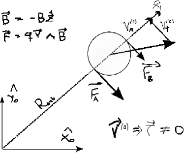
Figure 1: Under the action of a magnetic source in the origin, an orbital motion (in the radial direction, $v^{(o)}_{r}\neq 0$) generates a net torque $\mathbf{\tau}\neq 0$, due to the fact that $|\mathbf{F}_{A}|>|\mathbf{F}_{B}|$.

2) Figure 2. The distribution has no orbital motion now, but rotates around its center of symmetry. As a result of an angular velocity $\omega\neq 0$ (measured with respect to the inertial system $RF_{0}$), the Lorentz law induces forces in points $A$ and $B$, and all the points of the distribution. Again, because $|\mathbf{B}_{A}|>|\mathbf{B}_{B}|$, $|\mathbf{F}_{A}|>|\mathbf{F}_{B}|$, and (if we integrate for all points), there is a net resultant force acting on the mass center.

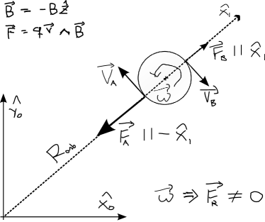
Figure 2: Under the action of a magnetic source in the origin, a self-rotational momentum $\mathbf{\omega}\neq 0$ originates a net resultant force $\mathbf{F}_{R}\neq 0$, modifying the orbit, due again to the fact that $|\mathbf{F}_{A}|>|\mathbf{F}_{B}|$.

Attention to sign consistency: from the graphical argument, we see that a positive (counterclockwise) angular velocity $\omega>0$ yields a negative force on the radial direction ($\mathbf{F}\cdot\hat{x}_{1}<0$, and a positive (outwards) radial velocity $v^{(o)}_{r}>0$ yields a positive (favors counter-clockwise rotation) torque ($\mathbf{\tau}\cdot\hat{z}_{0}>0$).

IV Quantitative analysis in 2D

IV.1 Reference frames

As before, we consider an inertial reference frame $RF_{0}$. The magnetic source stays attached to it, and the distribution moves. For convenience, we also consider a second system of reference $RF_{1}$, with its origin attached to the center of the distribution. The axes of $RF_{1}$ are not rigidly attached to the distribution, so there can be a net angular velocity $\boldsymbol{\omega}$ for $RF_{1}$ in respect to $RF_{0}$. Indeed, we will let it rotate around an axis of symmetry of the distribution. Moreover, $\mathbf{x}_{1}$, the x-axis of this system, $RF_{1}$, will be always aligned along the positive direction of the vector that joins the point-like source and the center of mass of the distribution. We therefore define, formally

$$\vec{R}_{orb}=-R_{orb}\ \mathbf{x}_{1},$$ (2)

The auxiliary system $RF_{1}$ will rotate instantaneously with angular velocity $\omega$ with respect to $RF_{0}$. Obviously, the fact that $RF_{1}$ can rotate in relation to $RF_{0}$ clearly excludes its inertiality. Nevertheless, we will express almost any vector in this frame $RF_{1}$. This is done for reasons of convenience.

Very important: this vector system $RF_{1}$ is only used as a reference in the mathematical sense, it is only a mathematical device. This means it is never used in the physical way: no force law (for instance, the Lorentz law), no mechanics (for instance, Newton’s second law) is ever evaluated in this frame. What we can do, however, is express any vector (any position, velocity, AM, force or torque) as referred to its basis vectors $\mathbf{x}_{1},\mathbf{y}_{1},\mathbf{z}_{1}$, which in turn are themselves functions of $\mathbf{x}_{0},\mathbf{y}_{0},\mathbf{z}_{0}$. This use of $RF_{1}$ will be very convenient to make the necessary changes that will allow to apply our picture to the more realistic situation of the hydrogen atom.

IV.2 Charge distribution

For the present work, we will consider a charge density $\rho(\mathbf{r}_{1})$ such that $\rho(\mathbf{r}_{1})>0$ only for $|\mathbf{r}_{1}|\leq R_{c}$, being the radius of the (spherical) distribution. We define a differential element of charge $dq=\rho(\mathbf{r}_{1})\ dv$, with $dv$ the differential element of volume.

IV.3 Purely kinematic considerations

For each differential element of the charge distribution, we have a velocity that we will divide in two components:

$$\mathbf{v}\ =\ \mathbf{v}^{(o)}\ +\ \mathbf{v}^{(R)}(\mathbf{r}_{1}),$$ (3)

where the superscript ’o’ will stand for “orbital” and ’R’ will stand for “rotational”. For convenience, we will write all expressions in terms of the versors of $RF_{1}$. This poses no problem as long as we regard $\mathbf{x}_{1},\mathbf{y}_{1},\mathbf{z}_{1}$ as functions of $\mathbf{x}_{0},\mathbf{y}_{0},\mathbf{z}_{0}$, and keep in mind $RF_{0}$ is our (only) inertial system. We will also include the dependence in $\mathbf{r}_{1}$ when this is indeed present, as we do in $\mathbf{v}^{(R)}(\mathbf{r}_{1})$. For the “orbital” component we will barely write $\mathbf{v}^{(o)}$, as we will see it is not dependent in $\mathbf{r}_{1}$. We define, for each differential element of charge in the distribution:

$$\mathbf{v}^{(o)}\ =\ v_{r}^{(o)}\ \mathbf{x}_{1}\ +\ v_{t}^{(o)}\ \mathbf{y}_{1},$$ (4)

with the components

$$\mathbf{v}^{(o)}_{t}=v^{(o)}_{t}\mathbf{x}_{1} = \boldsymbol{\omega}_{(o)}\ \wedge\ \vec{R}_{orb},$$ (5)

$$\mathbf{v}^{(o)}_{r}=v^{(o)}_{r}\mathbf{y}_{1} = \frac{d\vec{R}_{orb}}{dt},$$ (6)

where $\omega_{(o)}$ is defined by (5) as the angular velocity of $RF_{1}$ with respect to $RF_{0}$ and

$$\mathbf{v}^{(R)} = \boldsymbol{\omega}_{(R)}\ \wedge\ \mathbf{r}_{1},\ \ |\mathbf{r}_{1}|\leq R_{c},$$ (7)

with $\boldsymbol{\omega}_{(R)}=\omega_{(R)}\ \mathbf{z}_{1}$ (remember that in this section we restrict the initial conditions to the plane $OXY$), defined as

$$\omega_{(R)}=\omega-\omega_{(o)},$$ (8)

and $\omega$ is the angular velocity of the distribution with respect to $RF_{0}$ (see defs_omega ). Vectorially, $\boldsymbol{\omega}_{(R)}=\boldsymbol{\omega}-\boldsymbol{\omega}_{(o)}$, with the three vectors directed in the $\mathbf{z}_{1}\equiv\mathbf{z}_{0}$ axis. It is important to remark here that $\omega_{(R)}$, as defined above, is not an angular velocity as measured in $RF_{0}$, in contrast with $\omega$ and $\omega_{(o)}$. This definition of $\omega_{(R)}$ is justified for convenience, as it makes all our reasonings far more apparent. For clarification, and also because it will be useful, we add the following expression using spherical coordinates in $RF_{1}$:

$$\mathbf{v}^{(R)} = \omega_{(R)}r_{1}\sin\theta_{1}\ \left[\ \sin\psi_{1}\mathbf{x}_{1}-\cos\psi_{1}\mathbf{y}_{1}\ \right],$$ (9)

where $r_{1}=|\mathbf{r}_{1}|$ and $\omega_{(R)}$ is positive for a counter-clockwise rotation.

IV.4 Fields

We start by recalling that the electric field created by a point-like particle with charge $-q$ (electric monopole):

$$\mathbf{E}(\mathbf{r_{0}}) = -\frac{q}{4\pi\epsilon_{0}}\cdot\frac{\mathbf{r_{0}}}{|\mathbf{r_{0}}|^{3}},$$ (10)

but as a rule, we said we will express all in $RF_{1}$:

$$\mathbf{E}(\mathbf{r}_{1}) = -\frac{q}{4\pi\epsilon_{0}}\cdot\frac{(\mathbf{r}_{1}-R_{orb}\ \mathbf{x}_{1})}{|\mathbf{r}_{1}+R_{orb}\ \mathbf{x}_{1}|^{3}},$$ (11)

with $\mathbf{r_{0}}=\mathbf{r}_{1}+R_{orb}\ \mathbf{x}_{1}$, with $R_{orb}$ the orbital radius. Acting on each differential element of charge there is a purely electrostatic force:

$$d\mathbf{F}_{e} = dq(\mathbf{r}_{1})\ \mathbf{E}(\mathbf{r}_{1}),$$ (12)

and obviously

$$\mathbf{F}_{e}=\int{d\mathbf{F}_{e}}.$$ (13)

In the following we will face an analogous calculation with the Lorentz force. Here we have not developed (12)-(13) in a multipole expansion, as this would yield no special distinction among terms of a different nature. This will be, however, our main tool in the following calculations.

Now, the magnetic field created by a point-like magnetic dipole $\boldsymbol{\mu}=\mu\mathbf{z_{1}}$, if the source is sufficiently far to consider the observed field only has a $\mathbf{z}$ component:

$$\mathbf{B}(\mathbf{r}_{1}) = -B(\mathbf{r}_{1})\ \mathbf{z}_{1},$$ (14)

$$B(\mathbf{r}_{1}) = \hat{\mu}\ \frac{1}{|\mathbf{r}_{0}|^{3}}=\hat{\mu}\ \frac{1}{|\mathbf{r}_{1}+R_{orb}\ \mathbf{x}_{1}|^{3}},$$ (15)

defining the quantity $\hat{\mu}=\frac{\mu_{0}}{4\pi}\mu$, with $\mu>0$ the value of the magnetic moment of the point-like source.

IV.5 Multipole expansion

It is time to recall the first terms of a multipole expansion (around $\mathbf{r}_{0}=\vec{R}_{orb}$, or equivalently, $\mathbf{r}_{1}=O_{1}$):

$$\frac{1}{|\mathbf{r}_{0}|} = \frac{1}{|\mathbf{r}_{1}\ -\ (\ -\ R_{orb}\ \mathbf{x}_{1})|}$$ (16)

$$= \frac{1}{|\mathbf{r}_{1}+R_{orb}\ \mathbf{x}_{1}|}$$

$$= \frac{1}{R_{orb}}+\frac{(-R_{orb}\ \mathbf{x}_{1})\cdot\mathbf{r}_{1}}{R_{orb}^{3}}+\ldots$$

$$= \frac{1}{R_{orb}}-\frac{\mathbf{x}_{1}\cdot\mathbf{r}_{1}}{R_{orb}^{2}}+\ldots,$$

$$\frac{1}{|\mathbf{r}_{0}|^{2}} = \frac{1}{|\mathbf{r}_{1}\ -\ (\ -\ R_{orb}\ \mathbf{x}_{1})|^{2}}$$ (17)

$$= \frac{1}{|\mathbf{r}_{1}+R_{orb}\ \mathbf{x}_{1}|^{2}}$$

$$= \frac{1}{R_{orb}^{2}}+\frac{2(-R_{orb}\ \mathbf{x}_{1})\cdot\mathbf{r}_{1}}{R_{orb}^{4}}+\ldots$$

$$= \frac{1}{R_{orb}^{2}}-\frac{2\mathbf{x}_{1}\cdot\mathbf{r}_{1}}{R_{orb}^{3}}+\ldots,$$

$$\frac{1}{|\mathbf{r}_{0}|^{3}} = \frac{1}{|\mathbf{r}_{1}\ -\ (\ -\ R_{orb}\ \mathbf{x}_{1})|^{3}}$$ (18)

$$= \frac{1}{|\mathbf{r}_{1}+R_{orb}\ \mathbf{x}_{1}|^{3}}$$

$$= \frac{1}{R_{orb}^{3}}+\frac{3(-R_{orb}\ \mathbf{x}_{1})\cdot\mathbf{r}_{1}}{R_{orb}^{5}}+\ldots$$

$$= \frac{1}{R_{orb}^{3}}-\frac{3\mathbf{x}_{1}\cdot\mathbf{r}_{1}}{R_{orb}^{4}}+\ldots,$$

that we will now apply to the scalar $B(\mathbf{r}_{1})$, where $\mathbf{B}=B(\mathbf{r}_{1})\mathbf{z}_{1}$ is the magnetic field created by the point-like source:

$$B(\mathbf{r}_{1}) = \hat{\mu}\ \left[\frac{1}{R_{orb}^{3}}-\frac{3\ \mathbf{x}_{1}\cdot\mathbf{r}_{1}}{R_{orb}^{4}}+\ldots\right].$$

(19)

IV.6 On the electrostatic force

We already settled the expression for the purely electrostatic force in (12) and (13). That formula already accounts for the inclusion of higher order moments for the charge distribution. None of these terms, aside from introducing corrections to the overall magnitude of the resultant force $F_{e}$, adds any other effect from our point of view. In fact, there is no component of $F_{e}$ in the tangential ($\mathbf{y}_{1}$) direction, neither there is any kind of resultant torque over the center of mass of the distribution. For these reasons, we will not hereafter refer to this electrostatic term $F_{e}$, if it is not strictly necessary.

IV.7 Magnetic forces

From here on, we concentrate on the forces arising from the “second term” within the Lorentz force, that of the kind $q\mathbf{v}\ \wedge\ \mathbf{B}$. Acting on each differential element of charge, we have a force:

$$d\mathbf{F}_{m} = dq(\mathbf{r}_{1})\ \mathbf{v}(\mathbf{r}_{1})\ \wedge\ -B(\mathbf{r}_{1})\ \mathbf{z}_{1}$$

$$= dq(\mathbf{r}_{1})\ \left[\mathbf{v}^{(o)}+\mathbf{v}^{(R)}(\mathbf{r}_{1})\right]\wedge-B(\mathbf{r}_{1})\ \mathbf{z}_{1}.$$

(20)

where we have applied our decomposition in (3), and now we can write:

$$d\mathbf{F}_{m} = d\mathbf{F}_{m}^{(o)}\ +\ d\mathbf{F}_{m}^{(R)}.$$ (21)

defining:

$$d\mathbf{F}_{m}^{(o)} = dq(\mathbf{r}_{1})\ \mathbf{v}^{(o)}\wedge-B(\mathbf{r}_{1})\ \mathbf{z}_{1},$$ (22)

$$d\mathbf{F}_{m}^{(R)} = dq(\mathbf{r}_{1})\ \mathbf{v}^{(R)}(\mathbf{r}_{1})\ \wedge\ -B(\mathbf{r}_{1})\ \mathbf{z}_{1}.$$ (23)

IV.7.1 Orbital component

We start by analyzing the first of those two terms (a force from an “orbital” origin):

$$d\mathbf{F}_{m}^{(o)} = dq(\mathbf{r}_{1})\ \mathbf{v}^{(o)}\wedge-B(\mathbf{r}_{1})\ \mathbf{z}_{1}$$ (24)

$$= dq(\mathbf{r}_{1})\ \mathbf{v}^{(o)}\wedge$$

$$\quad-\hat{\mu}\ \left[\frac{1}{R_{orb}^{3}}-\frac{3\mathbf{x}_{1}\cdot\mathbf{r}_{1}}{R_{orb}^{4}}+\ldots\right]\ \mathbf{z}_{1},$$

and now, integrating for the whole distribution:

$$\mathbf{F}_{m}^{(o)} = \int{d\mathbf{F}_{m}^{(o)}},$$ (25)

and taking into account (19), we clearly see the first term (electric monopole) already gives the leading contribution to the integral, and therefore:

$$\mathbf{F}_{m}^{(o)} = \int{dq(\mathbf{r}_{1})\ \mathbf{v}^{(o)}\ \wedge\ \hat{\mu}\cdot\left[\frac{1}{R_{orb}^{3}}+\ldots\right]\ \mathbf{z}_{1}}$$ (26)

$$= (\mathbf{v}^{(o)}\ \wedge\ \mathbf{z}_{1})\cdot\frac{\hat{\mu}}{R_{orb}^{3}}\ \int{dq(\mathbf{r}_{1})}.$$

If we now isolate the leading order, defining:

$$\mathbf{F}_{m}^{(o)} \approx \frac{\hat{\mu}\ Q_{0}}{R_{orb}^{3}}\cdot(\mathbf{v}^{(o)}\ \wedge\ \mathbf{z}_{1}),$$ (27)

$$Q_{0} = \int{dq(\mathbf{r}_{1})},$$ (28)

where $Q_{0}$, a zero order moment of charge around $O_{1}$, i.e., $Q_{0}=q$, with $q>0$ the total charge of the distribution. Let us now use (4) and give a more detailed expression:

$$\mathbf{F}_{m}^{(o)}\approx\frac{\hat{\mu}\ q}{R_{orb}^{3}}\cdot\left[v^{(o)}_{t}\mathbf{x}_{1}-v^{(o)}_{r}\mathbf{y}_{1}\right],$$ (29)

though, in this case we could simply use the full order,

$$\mathbf{F}_{m}^{(o)} = |B(\mathbf{r}_{0}=\vec{R}_{orb})|\left[v^{(o)}_{t}\mathbf{x}_{1}-v^{(o)}_{r}\mathbf{y}_{1}\right]$$ (30)

$$= |B(\mathbf{r}_{1}=\mathbf{0})|\left[v^{(o)}_{t}\mathbf{x}_{1}-v^{(o)}_{r}\mathbf{y}_{1}\right].$$

IV.7.2 Rotational (“spinning”) component

Recalling (3), we set now the focus on $\mathbf{v}^{(R)}$,

$$d\mathbf{F}_{m}^{(R)} = dq(\mathbf{r}_{1})\ \mathbf{v}^{(R)}\ \wedge\ -B(\mathbf{r}_{1})\ \mathbf{z}_{1}$$

$$= dq(\mathbf{r}_{1})\ (\mathbf{\omega_{(R)}}\wedge\mathbf{r}_{1})\ \wedge\ -B(\mathbf{r}_{1})\ \mathbf{z}_{1}.$$

(31)

We can calculate a bit more:

$$d\mathbf{F}_{m}^{(R)} = dq(\mathbf{r}_{1})\ \omega_{(R)}\ \mathbf{z}_{1}\ \wedge\ \mathbf{r}_{1}\ \wedge\ -B(\mathbf{r}_{1})\ \mathbf{z}_{1}$$

$$= dq(\mathbf{r}_{1})\ \omega_{(R)}B(\mathbf{r}_{1})\ \mathbf{z}_{1}\ \wedge\ \mathbf{z}_{1}\ \wedge\ \mathbf{r}_{1}^{(h)}$$

$$= dq(\mathbf{r}_{1})\ \omega_{(R)}B(\mathbf{r}_{1})\ (-\mathbf{r}_{1}^{(h)})$$

$$= -\ dq(\mathbf{r}_{1})\ \omega_{(R)}B(\mathbf{r}_{1})\ \mathbf{r}_{1}^{(h)},$$

(32)

where each time we do $\mathbf{z}_{1}\ \wedge\$ on the left we “rotate” a 2D vector by an angle $\pi/2$ around the $\mathbf{z}$. We have also introduced, for a horizontal projection of a vector, the following notation, for any vector $\mathbf{A}$:

$$\mathbf{A}^{(h)} = (\mathbf{A}\cdot\mathbf{x}_{1})\ \mathbf{x}_{1}\ +\ (\mathbf{A}\cdot\mathbf{y}_{1})\ \mathbf{y}_{1},$$ (33)

$$\mathbf{A}^{(z)} = (\mathbf{A}\cdot\mathbf{z}_{1})\ \mathbf{z}_{1}.$$ (34)

We return to the integration now

$$\mathbf{F}_{m}^{(R)} = \int{d\mathbf{F}_{m}^{(R)}},$$ (35)

we can see the first term (19) gives rise to a contribution of first order to $\mathbf{F}_{m}^{(R)}$ (be aware of the last factor $\mathbf{r}_{1}^{(h)}$!), thus vanishing (as the dipolar electric moment of the distribution does). The second term in (19) gives rise, however, to a non vanishing contribution (as the second order moment does not vanish), due again to that last factor $\mathbf{r}_{1}^{(h)}$. We can then write:

$$\mathbf{F}_{m}^{(R)} = \int{dq(\mathbf{r}_{1})\ \omega_{(R)}\hat{\mu}\ \left[\ -\ \frac{3\mathbf{x}_{1}\cdot\mathbf{r}_{1}}{R_{orb}^{4}}+\ldots\right]\ (-\mathbf{r}_{1}^{(h)})}$$

$$= \int{dq(\mathbf{r}_{1})\ \omega_{(R)}\hat{\mu}\ \left[\frac{3\mathbf{x}_{1}\cdot\mathbf{r}_{1}}{R_{orb}^{4}}+\ldots\right]\ \mathbf{r}_{1}^{(h)}}$$

$$= \int{dq(\mathbf{r}_{1})\ \omega_{(R)}\hat{\mu}\ \left[\frac{3|\mathbf{r}_{1}^{(h)}|^{2}}{R_{orb}^{4}}+\ldots\right]\ \mathbf{x}_{1}}$$

$$= \omega_{(R)}\hat{\mu}\ \int{dq(\mathbf{r}_{1})\left[\frac{3|\mathbf{r}_{1}^{(h)}|^{2}}{R_{orb}^{4}}+\ldots\right]\ \mathbf{x}_{1}}$$

$$= \omega_{(R)}\hat{\mu}\ \int{dq(\mathbf{r}_{1})\left[\frac{3|\mathbf{r}_{1}^{(h)}|^{2}}{R_{orb}^{4}}+\ldots\right]\ \mathbf{x}_{1}},$$

(36)

where we have used $\vec{R}_{orb}=R_{orb}\ \mathbf{x}_{1}$. We now truncate to leading order, and solve the integral:

$$\mathbf{F}_{m}^{(R)} \approx \frac{3\hat{\mu}Q_{2}}{R_{orb}^{4}}\ \omega_{(R)}\ \mathbf{x}_{1},$$ (37)

where $Q_{2}$ is a second-order axial momentum around the $\mathbf{z}_{1}$-axis:

$$Q_{2} = \int{dq(\mathbf{r}_{1})\ |\mathbf{r}_{1}^{(h)}|^{2}}.$$ (38)

IV.7.3 Remarks

We remark that both $dF_{m}^{(o)},dF_{m}^{(R)}$, under these 2D initial conditions, only have components in the plane OXY:

$$\mathbf{F}_{m}=\int{(\ d\mathbf{F}_{m}^{(o)}+d\mathbf{F}_{m}^{(R)}\ )}=\int{d\mathbf{F}_{m}^{(h)}},$$ (39)

and we have also seen the first non vanishing term in both $dF_{m}^{(o)}$, in (25), and $dF_{m}^{(R)}$, (35), belongs, respectively, to zero and second order (desarrollar esto!!!).

IV.8 Magnetic torque

We analyze now the torque, that we previously introduced, from a very simple but intuitive graphical argument (reference to graphics). As a summary of this section, let us say we will show that this torque does indeed comes exclusively from the orbital movement, as we had already foreseen through the graphical argument. We define:

$$\boldsymbol{\tau}_{m}^{(o)} = \int{d\boldsymbol{\tau}_{m}^{(o)}},\quad d\boldsymbol{\tau}_{m}^{(o)}=\mathbf{r}_{1}\ \wedge\ d\mathbf{F}_{m}^{(o)},$$ (40)

$$\boldsymbol{\tau}_{m}^{(R)} = \int{d\boldsymbol{\tau}_{m}^{(R)}},\quad d\boldsymbol{\tau}_{m}^{(R)}=\mathbf{r}_{1}\ \wedge\ d\mathbf{F}_{m}^{(R)},$$ (41)

and obviously $\boldsymbol{\tau}_{m}=\boldsymbol{\tau}_{m}^{(o)}\ +\ \boldsymbol{\tau}_{m}^{(R)}$.

IV.8.1 Orbital component

Using (22) we have

$$d\boldsymbol{\tau}_{m}^{(o)} = \mathbf{r}_{1}\ \wedge\ d\mathbf{F}_{m}^{(o)}$$ (42)

$$= \mathbf{r}_{1}\ \wedge\ dq(\mathbf{r}_{1})\ \left[\ \mathbf{v}^{(o)}\wedge-B(\mathbf{r}_{1})\ \mathbf{z}_{1}\ \right].$$

Now, with $\mathbf{v}^{(o)}=v^{(o)}_{r}\mathbf{x}_{1}+v^{(o)}_{t}\mathbf{y}_{1}$ because our planar initial condition, we do

$$d\boldsymbol{\tau}_{m}^{(o)} = \mathbf{r}_{1}\ \wedge\ dq(\mathbf{r}_{1})\ \left[\ v_{r}^{(o)}\ \mathbf{x}_{1}+v_{t}^{(o)}\ \mathbf{y}_{1}\ \right]\wedge-B(\mathbf{r}_{1})\ \mathbf{z}_{1}$$

$$= dq(\mathbf{r}_{1})\ B(\mathbf{r}_{1})\ \mathbf{r}_{1}\ \wedge\ (-v_{r}^{(o)}\ \mathbf{y}_{1}\ +\ v_{t}^{(o)}\ \mathbf{x}_{1}),$$

(43)

Also, due to reflection symmetry around the OXY plane, all contributions to $\boldsymbol{\tau}_{m}^{(o)}$ in that plane vanish when integrated:

$$\boldsymbol{\tau}_{m}^{(o)}=\int{d\boldsymbol{\tau}_{m}^{(o)}}=\int{(d\boldsymbol{\tau}_{m}^{(o)})^{(z)}},$$ (44)

and using (42) we do

$$d\boldsymbol{\tau}_{m}^{(o)} = \mathbf{r}_{1}\ \wedge\ dq(\mathbf{r}_{1})\ \left[\ -\mathbf{v}^{(o)}\ \wedge\ -B(\mathbf{r}_{1})\ \mathbf{z}_{1}\ \right]$$ (45)

$$= \mathbf{v}^{(o)}\ \wedge\ dq(\mathbf{r}_{1})\ \mathbf{r}_{1}\ \wedge\ -B(\mathbf{r}_{1})\ \mathbf{z}_{1}$$

$$= -\mathbf{v}^{(o)}\ \wedge\ dq(\mathbf{r}_{1})\ \mathbf{r}_{1}^{(h)}\ \wedge\ B(\mathbf{r}_{1})\ \mathbf{z}_{1},$$

and applying the multipole expansion for the magnetic field (19),

$$d\boldsymbol{\tau}_{m}^{(o)}=-\mathbf{v}^{(o)}\ \wedge\ dq(\mathbf{r}_{1})\ \times\$$

$$\quad\quad\quad(\ \mathbf{r}_{1}^{(h)}\ \wedge\ \hat{\mu}\ \left[\frac{1}{R_{orb}^{3}}-\frac{3\mathbf{x}_{1}\cdot\mathbf{r}_{1}}{R_{orb}^{4}}+\ldots\right]\ \mathbf{z}_{1}\ ),$$

With the “additional” factor $\mathbf{r}_{1}^{(h)}$, the first term of the expansion goes from zero to second order. Clearly it gives no net contribution to the integral. The second term goes from first to second order, and it is the leading contribution. Keeping this leading term and truncating:

$$d\boldsymbol{\tau}_{m}^{(o)} \approx -\mathbf{v}^{(o)}\wedge\ dq(\mathbf{r}_{1})\ \mathbf{r}_{1}^{(h)}\wedge\ \hat{\mu}\ \frac{3\mathbf{x}_{1}\cdot\mathbf{r}_{1}}{R_{orb}^{4}}\ \mathbf{z}_{1}$$

$$= -\ \mathbf{v}^{(o)}\wedge\ dq(\mathbf{r}_{1})\ \mathbf{r}_{1}^{(h)}\wedge\ \hat{\mu}\ \frac{3\mathbf{x}_{1}\cdot\mathbf{r}_{1}}{R_{orb}^{4}}\ \mathbf{z}_{1}$$

$$= \-\mathbf{v}^{(o)}\wedge\ \hat{\mu}\ dq(\mathbf{r}_{1})\ \frac{3|\mathbf{r}_{1}^{(h)}|^{2}\ \cos\psi_{1}}{R_{orb}^{4}}$$

$$\ \ \ \ \ \ \ \ \ \ \ \ \ \ \ \ \ \ \ \ \ \ \ \ \times\ (\ \sin\psi_{1}\mathbf{x}_{1}-\cos\psi_{1}\mathbf{y}_{1}\ )$$

$$= \-\mathbf{v}^{(o)}\ \wedge\ \hat{\mu}\ dq(\mathbf{r}_{1})\ \frac{3|\mathbf{r}_{1}^{(h)}|^{2}}{R_{orb}^{4}}$$

$$\ \ \ \ \ \ \ \ \ \ \ \ \ \ \ \times\ (\ \sin\psi_{1}\cos\psi_{1}\mathbf{x}_{1}-\cos^{2}\psi_{1}\mathbf{y}_{1}\ ),$$

We could not avoid having to invoke explicitly some coordinates here, $\phi_{1}$ being the azimuthal angle in system 1. The term in $\sin\phi_{1}\cos\phi_{1}$ clearly vanishes if we integrate for $\psi\in[0,2\pi]$, but no the one in $\cos^{2}\psi_{1}$, and finally:

$$\boldsymbol{\tau}_{m}^{(o)} \approx \int{\mathbf{v}^{(o)}\ \wedge\ \hat{\mu}\ dq(\mathbf{r}_{1})\ \frac{3|\mathbf{r}_{1}^{(h)}|^{2}\ \cos^{2}\psi_{1}}{R_{orb}^{4}}\ \mathbf{y}_{1}}$$

$$= \mathbf{v}^{(o)}\ \wedge\ \frac{3\hat{\mu}}{R_{orb}^{4}}\cdot\int{dq(\mathbf{r}_{1})\ |\mathbf{r}_{1}^{(h)}|^{2}\cos^{2}\psi_{1}}\ \mathbf{y}_{1}$$

$$= \mathbf{v}^{(o)}\ \wedge\ \frac{3\hat{\mu}Q_{2}^{(*)}}{R_{orb}^{4}}\ \mathbf{y}_{1}$$

$$= \frac{3\hat{\mu}Q_{2}^{(*)}}{R_{orb}^{4}}\ \mathbf{y}_{1}\ \wedge\ \mathbf{v}^{(o)}=\frac{3\hat{\mu}Q_{2}^{(*)}}{R_{orb}^{4}}\cdot v_{r}^{(o)}\ \mathbf{z}_{1},$$

(48)

in the $z$-direction, as expected, and where

$$Q_{2}^{(*)}=\int{dq(\mathbf{r}_{1})\cdot|\mathbf{r}_{1}^{(h)}|^{2}\cos^{2}\psi_{1}},$$ (49)

is a second order axial moment of the distribution (we have to check this calculations).

IV.8.2 Rotational component

Now we analyze $d\boldsymbol{\tau}_{m}^{(R)}$, and we prove that $\boldsymbol{\tau}_{m}^{(R)}=0$, i.e., the only contribution to this torque of magnetic origin comes from the orbital term. We see:

$$d\boldsymbol{\tau}_{m}^{(R)} = \mathbf{r}_{1}\ \wedge\ d\mathbf{F}_{m}^{(R)}$$ (50)

$$= \mathbf{r}_{1}\ \wedge\ dq(\mathbf{r}_{1})\ (\ \mathbf{v}^{(R)}\ \wedge\ -B(\mathbf{r}_{1})\ \mathbf{z}_{1}\ )$$

$$= dq(\mathbf{r}_{1})\ \mathbf{r}_{1}\ \wedge\ (\mathbf{\omega_{(R)}}\ \wedge\ \mathbf{r}_{1})\ \wedge\ -B(\mathbf{r}_{1})\ \mathbf{z}_{1}$$

$$= dq(\mathbf{r}_{1})\ \mathbf{r}_{1}\ \wedge\ \omega_{(R)}\mathbf{z}_{1}\ \wedge\ B(\mathbf{r}_{1})\ \mathbf{z}_{1}\ \wedge\ \mathbf{r}_{1}$$

$$= dq(\mathbf{r}_{1})\ \mathbf{r}_{1}\ \wedge\ \omega_{(R)}B(\mathbf{r}_{1})\ \wedge\ (-\mathbf{r}_{1}^{(h)})$$

$$= dq(\mathbf{r}_{1})\ \omega_{(R)}B(\mathbf{r}_{1})\ \mathbf{r}_{1}^{(h)}\ \wedge\ -\mathbf{r}_{1}^{(h)}$$

$$= -dq(\mathbf{r}_{1})\ \omega_{(R)}B(\mathbf{r}_{1})\ \mathbf{r}_{1}^{(h)}\ \wedge\ \mathbf{r}_{1}^{(h)}$$

$$= 0.$$

Therefore,

$$\boldsymbol{\tau}_{m}^{(R)}=\int{d\boldsymbol{\tau}_{m}^{(R)}}=0.$$ (51)

It is worth to remark this last result: the torque on the z-direction (to be applied on the center of mass of the distribution of charge), comes exclusively from the “orbital” contribution, that contribution with origin in the “orbital” AM of the distribution as a point particle (therefore, represented by a center of mass).

IV.9 Summary of results for the 2-dimensional problem

The following shows the first contribution in the electrical multipole expansion for each of the forces or torques. To second order (Q), no other forces or rotational momenta arise.

Order	$\mathbf{F}_{m}^{(o)}$	$\mathbf{F}_{m}^{(R)}$	$\boldsymbol{\tau}_{m}^{(o)}$	$\boldsymbol{\tau}_{m}^{(R)}$
Zero (M)	$Yes$	$No$	$No$	$No$
First (D)	$Yes$	$No$	$No^{\ast}$	$No$
Second (Q)	$Yes$	$Yes$	$Yes$	$No$

A table of dependencies may be of use, too,

Variable	$\mathbf{F}_{m}^{(o)}$	$\mathbf{F}_{m}^{(R)}$	$\boldsymbol{\tau}_{m}^{(o)}$	$\boldsymbol{\tau}_{m}^{(R)}$
$|R_{orb}|^{-1}$	$Yes$	$Yes$	$Yes$	$-$
$\omega_{(R)}$	$-$	$Yes$	$-$	$-$
$v^{(o)}_{r}$	$Yes$	$-$	$Yes$	$-$
$v^{(o)}_{t}$	$Yes$	$-$	$-$	$-$

IV.10 3D initial conditions

We have a 3D extension of the problem. Here, $\mathbf{x}_{1}$ still goes in the radial direction of the orbit, $\mathbf{y}_{1}$ in the tangential direction and $\mathbf{z}_{1}$ is always the instantaneous axis for $\omega_{(o)}$. We have now:

$$\mathbf{v}^{(o)} = v_{r}^{(o)}\mathbf{x}_{1}\ +\ v_{t}^{(o)}\mathbf{y}_{1}\ +\ v_{z}^{(o)}\mathbf{z}_{1},$$ (52)

and

$$\boldsymbol{\omega}_{(R)} = (\omega_{(R)})_{r}\ \mathbf{x}_{1}+(\omega_{(R)})_{t}\ \mathbf{y}_{1}+(\omega_{(R)})_{z}\ \mathbf{z}_{1},$$

(53)

with, now, vectorially (recall Sec. IV.3),

$$\boldsymbol{\omega}_{(R)}=\boldsymbol{\omega}-\boldsymbol{\omega}_{(o)},$$ (54)

Needless to say, we can always decompose the dynamics of the system in this way. Now we complete the systematic analysis of the dominant terms for the forces, $\mathbf{F}_{m}^{(o)},\mathbf{F}_{m}^{(R)}$, and torques, $\boldsymbol{\tau}_{m}^{(o)},\boldsymbol{\tau}_{m}^{(R)}$. First we calculate the new contributions to the forces:

$$\Delta(d\mathbf{F}_{m}^{(o)}) = dq(\mathbf{r}_{1})\ v_{z}^{(o)}\mathbf{z}_{1}\ \wedge\ -B(\mathbf{r}_{1})\ \mathbf{z}_{1}=0,$$

(55)

so there is no new contribution to $\mathbf{F}_{m}^{(o)}$, and

$$\Delta(d\mathbf{F}_{m}^{(R)}) = dq(\mathbf{r}_{1})\ (\boldsymbol{\omega}_{(R)})^{(h)}\ \wedge\ \mathbf{r}_{1}\ \wedge\ -B(\mathbf{r}_{1})\ \mathbf{z}_{1}$$

$$= -\ dq(\mathbf{r}_{1})\ B(\mathbf{r}_{1})\ (\boldsymbol{\omega}_{(R)})^{(h)}\ \wedge\ \mathbf{r}_{1}\ \wedge\ \mathbf{z}_{1}$$

$$= \Delta(d\mathbf{F}_{m}^{(R)})^{(z)}.$$

(56)

This is rewarding because the new contribution is normal to the one we already have. We can also write

$$\Delta(d\mathbf{F}_{m}^{(R)})=dq(\mathbf{r}_{1})\ B(\mathbf{r}_{1})\ (\boldsymbol{\omega}_{(R)})^{(h)}\ \wedge\ \mathbf{r}_{1}^{(h,\pi/2)},$$ (57)

where $\mathbf{r}_{1}^{(h,\pi/2)}$ stands for a rotation of $\mathbf{r}_{1}^{(h)}$ by an angle $\pi/2$ around the z-axis. We would have the integral

$$\Delta(\mathbf{F}_{m}) = \int{\Delta(d\mathbf{F}_{m})}$$ (58)

$$= \int{\Delta(d\mathbf{F}_{m}^{(o)})}+\int{\Delta(d\mathbf{F}_{m}^{(R)})}$$

$$= \int{\Delta(d\mathbf{F}_{m}^{(R)})^{(z)}}\ =\ \Delta(\mathbf{F}_{m}^{(R)})^{(z)},$$

where we have just identified that $\mathbf{F}_{m}^{(R)}$ only has a component in the $z$-direction. Now we see the new components for the torques. Clearly from (55) we see there is neither any new contribution to the part of the torque that originates from the “orbital” movement:

$$\Delta(d\boldsymbol{\tau}_{m}^{(o)}) = \mathbf{r}_{1}\ \wedge\ \Delta(d\mathbf{F}_{m}^{(o)})=0,$$ (59)

and for the rotational part, using that $\Delta(d\mathbf{F}_{m}^{(R)})=\Delta(d\mathbf{F}_{m}^{(R)})^{(z)}$, we can write

$$\Delta(d\boldsymbol{\tau}_{m}^{(R)}) = \mathbf{r}_{1}\ \wedge\ \Delta(d\mathbf{F}_{m}^{(R)})$$

$$= \mathbf{r}_{1}\ \wedge\ \Delta(d\mathbf{F}_{m}^{(R)})^{(z)}$$

$$= \mathbf{r}_{1}^{(h)}\wedge\ \Delta(d\mathbf{F}_{m}^{(R)})^{(z)}\ =\ (\Delta d\boldsymbol{\tau}_{m}^{(R)})^{(h)},$$

(60)

again with the rewarding result that this new contribution $\Delta(d\boldsymbol{\tau}_{m}^{(R)})$ is a “horizontal” vector (vector in the plane OXY) and hence normal to the contribution we already had for the “planar” initial conditions.

Again we attempt to summarize everything in a table. These results are generalized to any -planar or not- initial conditions. First line says whether a net contribution exists. Second line establishes a dependence. Last line says which is the leading order: zero (M), first (D) or second (Q).

$\mathbf{F}_{m}^{(o,h)}$	$\mathbf{F}_{m}^{(o,z)}$	$\mathbf{F}_{m}^{(R,h)}$	$\mathbf{F}_{m}^{(R,z)}$	$\boldsymbol{\tau}_{m}^{(o,h)}$	$\boldsymbol{\tau}_{m}^{(o,z)}$	$\boldsymbol{\tau}_{m}^{(R,h)}$	$\boldsymbol{\tau}_{m}^{(R,z)}$
$Yes$	$-$	$Yes$	$Yes$	$-$	$Yes$	$Yes$	$-$
$v_{r}^{(o)}$	$-$	$(\omega_{(R)})^{(z)}$	$(\boldsymbol{\omega}_{(R)})^{(h)}$	$-$	$v_{r}^{(o)}$	$(\boldsymbol{\omega}_{(R)})^{(h)}$	$-$
$M$	$-$	$Q$	$Q$	$-$	$Q$	$Q$	$-$

On the other hand, the new terms should correspond to what is known as the classical counterpart of the quantum LS or spin-orbit coupling. This interaction is also a stabilizing one, as it tends to keep parallel the spinning axis of particle and the axis of the orbit (the direction of the dipoling source). Nevertheless, for the moment we will only pay limited attention to questions regarding the problem in 3D.

V Towards a realistic model of the H-atom: relocation of mass

We had begun presenting an idealized electromechanical game. Now we establish a bridge from that situation to a realistic model for the classical H-atom. This implies a relocation of the inertial system, and a proof that the equations of the system remain the same in the new situation. Later, the value of the parameters in the model must be adjusted to resemble the actual charges, masses, etc of the hydrogen atom, but this will not be, for convenience, done yet.

V.1 Relocation of mass

In this section we do a relocation of the inertial frame of reference, $RF_{0}$. To indicate this we introduce the notation $RF_{0}|^{(n)}$, in contrast to $RF_{0}|^{(old)}$. If our situation is to resemble reasonably the real hydrogen atom, a natural choice is to attach $RF_{0}|^{(n)}$ to the center of the proton (the charge distribution), taking advantage from its much higher mass in respect to the electron. Still, the proton can “rotate” around $\mathbf{z}_{0}$ (on the planar problem), with angular velocity

$$\omega|^{(n)}=\omega_{(R)}|^{(n)}+\omega_{(o)}|^{(n)},$$ (61)

with respect to $RF_{0}|^{(n)}$. This definition is consistent with the one already given in (8), so, analogously to what happened there, $\omega|^{(n)}$ and $\omega_{(o)}|^{(n)}$ both have an “inertial” meaning (they are both angular frequencies measured with respect to an inertial reference frame $RF_{0}$), while $\omega_{(R)}|^{(n)}$ does not (but is nevertheless a very convenient dynamical variable from the point of view of the equations and our whole argument). Of course, we are only dealing here with the 2-dimensional situation: for the 3D problem, the same would hold but vectorially this time (it is always possible to decompose the (instantaneous) movement this way): $\boldsymbol{\omega}|^{(n)}=\boldsymbol{\omega}_{(R)}|^{(n)}+\boldsymbol{\omega}_{(o)}|^{(n)}$.

Again, an auxiliary system $RF_{1}|^{(n)}$ is of good use. We choose to attach it, as we did before, to the center of the distribution, and also choose the same orientation, so that $RF_{1}|^{(n)}\equiv RF_{1}|^{(old)}$ (hence we simply write $RF_{1}$), but this time, also, the origin $RF_{1}|^{(n)}$ and $RF_{0}|^{(n)}$ is common.

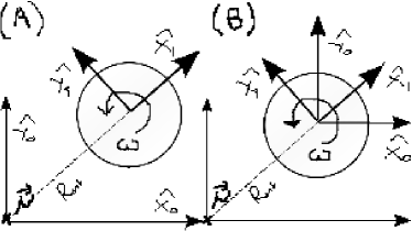
Figure 3: Location of systems $RF_{0}$ and $RF_{1}$ in situation (A) and (B). In (A), origin of $RF_{0}$ coincides with the position of the magnetic point-like dipole $\boldsymbol{\mu}$, while in (B) both origins coincide.

On the other hand, the point-like magnetic source (an electron, here) will orbit with velocity $\mathbf{v}^{(o)}|^{(n)}=\mathbf{v}^{(o)}_{t}|^{(n)}+\mathbf{v}^{(o)}_{r}|^{(n)}$ around the proton, and, again in this situation, the components can be expressed using the versors of $RF_{1}$, in the way:

$$\mathbf{v}^{(o)}_{r}|_{(n)} = v^{(o)}_{r}|_{(n)}\ \mathbf{x}_{1},$$ (62)

$$\mathbf{v}^{(o)}_{t}|_{(n)} = v^{(o)}_{t}|_{(n)}\ \mathbf{y}_{1}.$$ (63)

V.2 Formal equivalence of the equations

The problem of a moving magnetic dipole is a classical one in electromagnetism. Due to Lorentz covariance, a magnetic dipole $\boldsymbol{\mu}$ that moves with velocity $\mathbf{v}$ in respect to an inertial frame is seen, by an observer in that inertial frame, as an electrical dipole of value $\mathbf{p}$ proportional to $\boldsymbol{\mu}\wedge\mathbf{v}$. For more details in this result, we can cite , for instance, Panofsky_Philips (18-5, page 334). This electric “effective” dipole creates, at the point $\mathbf{r}_{0}=R_{orb}\ \mathbf{x}_{1}+\mathbf{r}_{1}$, an electric field

$$\mathbf{E}|_{(n)}\ \propto \frac{\mathbf{p}}{|R_{orb}\ \mathbf{x}_{1}+\mathbf{r}_{1}|^{3}}=\frac{\boldsymbol{\mu}\wedge\mathbf{v}|_{(n)}}{|R_{orb}\ \mathbf{x}_{1}+\mathbf{r}_{1}|^{3}},$$ (64)

therefore exerting a force

$$d\mathbf{F}|_{(n)}\ =\ dq\ \mathbf{E}|_{(n)}\ \propto\ dq\frac{\boldsymbol{\mu}\wedge\mathbf{v}|_{(n)}}{|R_{orb}\ \mathbf{x}_{1}+\mathbf{r}_{1}|^{3}},$$ (65)

on every element of charge $dq$ of the distribution. Now, we recall that in our previous situation we had, sufficiently away from the source,

$$\mathbf{B}|_{(old)}\ \approx\frac{\mu_{0}}{4\pi}\times\frac{\boldsymbol{\mu}}{|R_{orb}\ \mathbf{x}_{1}+\mathbf{r}_{1}|^{3}},$$ (66)

and therefore

$$d\mathbf{F}|_{(old)} = dq\frac{\mathbf{v}|_{(old)}\wedge\mathbf{B}|_{(old)}}{R_{orb}^{3}}=dq\frac{\mathbf{v}|_{(old)}\wedge\boldsymbol{\mu}}{|R_{orb}\ \mathbf{x}_{1}+\mathbf{r}_{1}|^{3}}.$$

(67)

But now is the source that moves in respect to the element of charge $dq$. Clearly, $\mathbf{v}|_{(n)}=-\mathbf{v}|_{(old)}$. Moreover, for clarity we also state:

$$\mathbf{v}^{(o)}|_{(n)} = -\mathbf{v}^{(o)}|_{(old)},$$ (68)

$$\mathbf{v}^{(R)}|_{(n)} = -\mathbf{v}^{(R)}|_{(old)},$$ (69)

and also clearly,

$$\omega_{(R)}|^{(n)} = \omega_{(R)}|^{(n)}.$$ (70)

But it does suffice to perform the substitution $\mathbf{v}|_{(n)}=-\mathbf{v}|_{(old)}$ in (65), and so we have, again,

$$d\mathbf{F}|_{(n)}\ \ \propto\ dq\frac{\mathbf{v}|_{(old)}\wedge\boldsymbol{\mu}}{|R_{orb}\ \mathbf{x}_{1}+\mathbf{r}_{1}|^{3}},$$ (71)

This is the same as we had in (67) and so it was exactly what we were looking for.

Therefore, at least for the term that depends on a wedge product on the velocity vector, the expression of the force $\mathbf{F}$ on each element of charge is completely equivalent (modulus a certain constant) to the one in our previous situation, the first electromechanical model we presented here. Moreover, all previous expressions are applicable (modulus a possible constant), and no further changes needed, as we take advantage here of the fact that all of them were referred to $RF_{1}$, that has not changed in the new picture (using this trick has saved us a lot of calculations).

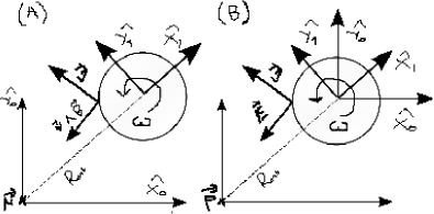
Figure 4: Direction of the force in situation (A): $\mathbf{dF}=dq\mathbf{v}\wedge\mathbf{B}$, and (B): $dF=dq\mathbf{E}$. From $RF_{0}$, the magnetic dipole $\boldsymbol{\mu}$ is seen as an electric dipole $\mathbf{p}$, source of the corresponding electric field.

VI Dynamical equations (2D)

We have seen that the equations of the system are invariant about whether it is the point-like negative charge or the extended distribution (of positive charge) that is moving, if we do the convenient redefinition of velocities. Using that fact, we present a first set of equations, that will be later enhanced by the inclusion of the radiative correction as well as the absorption from the background. This second step is done, anyway, only in an “approximate” way that is nevertheless enough for our purposes.

VI.1 Dynamical equations in absence of rad/abs

In the following equations, all quantities ($q$, $E_{1}$, $B_{1}$, etc.) are defined positive. In absence of dissipation and absorption and for the planar problem, the dynamical equations of the system are, to leading order,

(correction from previous version in first equation - originally it was correct in rest of the paper though)

$$m\ \dot{v}^{(o)}_{r}+m\frac{(v^{(o)}_{t})^{2}}{R_{orb}}\approx\left[\ \mathbf{F}_{e}\ +\ \mathbf{F}_{m}^{(o)}\ +\ \mathbf{F}_{m}^{(R)}\ \right]\cdot\mathbf{x}_{1}$$

$$\quad\quad\quad\quad=\ -\ qE_{1}\ -\ qB_{1}\ v^{(o)}_{t}\ -\ \frac{3\hat{\mu}Q_{2}}{R_{orb}^{4}}\ \omega_{(R)},$$

(72)

$$m\ \dot{v}^{(o)}_{t} \approx \left[\ \mathbf{F}_{m}^{(o)}\ +\ \mathbf{F}_{m}^{(R)}\ \right]\cdot\mathbf{y}_{1}=\mathbf{F}_{m}^{(o)}\cdot\mathbf{y}_{1}$$ (73)

$$= \ +\ qB_{1}\ v^{(o)}_{r},$$

$$M_{2}\ \dot{\omega_{(R)}} \approx \boldsymbol{\tau}_{m}^{(o)}\cdot\mathbf{z}_{1}\ +\ \boldsymbol{\tau}_{m}^{(R)}\cdot\mathbf{z}_{1}=\boldsymbol{\tau}_{m}^{(o)}\cdot\mathbf{z}_{1}$$ (74)

$$= \ +\ \frac{3\hat{\mu}\ Q_{2}^{(*)}}{R_{orb}^{4}}\ v^{(o)}_{r},$$

with $M_{2}$ a mass second order moment or “inertia” moment. In the first of the former equations (72), we take into account the fact that $RF_{1}$ is rotating with respect to $RF_{0}$, and that we have defined this radial velocity as $v^{(o)}_{r}=v^{(o)}_{r}\ \mathbf{x}_{1}$.

As a clarification, we recall $\mathbf{F}_{m}^{(R)}$ has no component in $\mathbf{y}_{1}$. Also, we have to notice $E_{1}$, $B_{1}$ do depend on $R_{orb}$ (see below). To the former three equations, we must add the obvious

$$\dot{R}_{orb} = {v}^{(o)}_{r},$$ (75)

and they must also be supplemented with the values of two fields evaluated in $\mathbf{r}_{1}=0$. With $\mathbf{E}(\mathbf{r}_{1})=-E(\mathbf{r}_{1})\ \mathbf{x}_{1}$ and $\mathbf{B}(\mathbf{r}_{1})=-B(\mathbf{r}_{1})\ \mathbf{z}_{1}$, we have

$$E_{1} = |\mathbf{E}(\mathbf{r}_{1})|=+\frac{q}{4\pi\epsilon_{0}\ R_{orb}^{2}},$$ (76)

$$B_{1} = |\mathbf{B}(\mathbf{r}_{1})|\propto+\ \frac{\mu_{0}}{4\pi}\frac{\mu_{e}}{R_{orb}^{3}},$$ (77)

with $\mu_{e}$ the magnetic dipole moment of the electron. Note: we can just state proportionality in the last equation as there are additional factors due to our “mass relocation”; anyway the contribution of $B_{1}$ is marginal and without implications for stability, we will even ignore it a future revision, just as some other terms - for instance the classical counterpart of the LS quantum term - are also ignored in these basic sets of equations).

See (11)-(15). It is important to note that these fields enter the former equations with the values in the point $\mathbf{r}_{0}=\vec{R}_{orb}$ (i.e., $\mathbf{r}_{1}=0$). To leading order, then, any other information about the distribution is already contained in $q$, $Q_{2}$ and $Q_{2}^{*}$. The first moment $Q_{1}=0$ vanishes, as all charges in the distribution are of equal sign, and moments of higher order are not considered.

VI.2 Inclusion of rad/abs

How do we include the radiative correction? From the point of view of the equations, it would suffice to include a stochastic term in (72), (73), and possibly in (74). This stochastic term represents the difference of loss and absorbed radiation in each instant of time, and its mean value is zero for a stationary orbit (an “attractor”). For non stationary orbits the mean value of this stochastic term would not be zero.

The inclusion in (72), (73) is quite obvious: we must allow for an energy loss through a fall of the orbital radius and a decrement of the modulus of the tangential velocity. The term in (74) is not so obvious, and we will extend on this later. On the other hand, a more rigorous treatment is not necessary for our purposes, at least for now.

VI.2.1 Rad/abs for a circular orbit

Puthoff calculated $\langle P_{ab}\rangle_{(orbit)}$ assuming statistical equilibrium with the orbital degrees of freedom (these are the two spatial coordinates in the plane, oscillating with frequency $\omega_{(o)}$, so therefore they can be seen as two one-dimensional harmonic oscillators in quadrature). Following Puthoff87 , we had

$$\langle P_{rad}\rangle_{(circ)}=\frac{q^{2}R_{orb}^{2}\omega_{(o)}^{4}}{6\pi\epsilon_{0}c^{3}},$$ (78)

which is directly obtainable from the Larmor formula with acceleration

$$\dot{v}^{(o)}_{r}=\frac{(v^{(o)}_{t})^{2}}{R_{orb}}=\omega_{(o)}^{2}R_{orb},$$ (79)

and

$$\langle P_{ab}\rangle_{(circ)}=\frac{q^{2}\hbar\omega_{(o)}^{3}}{6\pi\epsilon_{0}mc^{3}},$$ (80)

But here we deal with an instantaneous basis: the particle will suffer the action of a field with an stochastic instantaneous value (the ZPF), and will also loose energy whose (expectation?) (instantaneous) value is given by the radiation term (dependent on the instantaneous velocity).

VI.2.2 Rad/abs for the radial component

To first approximation, we can introduce a correction just in (72), through the inclusion of an stochastic term $\chi_{r}$, with an expectation value which depends on $R_{orb}$, and must change sign around the “stable” value $R_{orb}^{st}$. This $R_{orb}^{st}$ is the value of $R_{orb}$ for which the balance, on average over a cyclic orbit, of loss and absorption takes place, i.e., an equality between eqs. (80) and (78) holds. So,

$$\langle\chi_{r}(R_{orb})\rangle<0,\quad R_{orb}>R_{orb}^{st},$$ (81)

$$\langle\chi_{r}(R_{orb})\rangle>0,\quad R_{orb}<R_{orb}^{st},$$ (82)

for example,

$$\langle\chi_{r}(R_{orb})\rangle\approx k_{r}(R_{orb}^{st}-R_{orb}),\quad k_{r}>0.$$ (83)

For clarification, we have to say that the instantaneous values of $P_{ab}$ and $P_{rad}$ are stochastic variables whose distributions depend on the instantaneous values of $R_{orb}$, $v^{(o)}_{r}$, etc., and therefore, strictly speaking $\chi(R_{orb})=f\left(P_{ab}-P_{rad}\right)$, and (83) is only justified for mean values (which is what we have done).

VI.2.3 Rad/abs for the tangential component

Moreover, the gain/loss of energy affects both the radial and tangential components of the velocity. For this reason, we consider a second stochastic component $\chi_{t}(R_{orb})$, satisfying, this time

$$\langle\chi_{t}(v^{(o)}_{t})\rangle<0,\quad v^{(o)}_{t}>v^{(o)}_{t}|_{st},$$ (84)

$$\langle\chi_{t}(v^{(o)}_{t})\rangle>0,\quad v^{(o)}_{t}<v^{(o)}_{t}|_{st},$$ (85)

and therefore, close to the point of equilibrium $v^{(o)}_{t}|_{st}$, we can write

$$\langle\chi_{t}(v^{(o)}_{t})\rangle\approx k_{t}(v^{(o)}_{t}|_{st}-v^{(o)}_{t}),\quad k_{t}>0.$$ (86)

VI.2.4 Rad/abs due to “spinning”

Our study of the dynamical equations lead us to conclude that we need another dissipation/gain loss for the degree of freedom represented by $\omega$. The rotational movement of the distribution around an axis is also subjected to loss and absorption from the background. In the way we have done before, we write

$$\langle\chi_{\omega}(\omega)\rangle\approx k_{\omega}(\omega^{st}-\omega),\quad k_{\omega}>0.$$ (87)

Naturally, for a realistic hydrogen atom we would have $\omega|^{st}=0$ (the proton is quasi-attached to an inertial system: it can oscillate with respect to it, but the mean value of this oscillation is zero). We will comment on this later.

VI.2.5 Complete dynamical equations

We now include all the former corrections in the dynamical equations of the system. First, for the radial component:

$$m\dot{v}^{(o)}_{r} + m\ \frac{(v^{(o)}_{t})^{2}}{R_{orb}}\approx$$

$$-qE_{1}-qB_{1}\ v^{(o)}_{t}-\frac{3\hat{\mu}Q_{2}}{R_{orb}^{4}}\ \omega_{(R)}+\chi_{r},$$

(88)

and reordering (that term on the left…),

$$m\dot{v}^{(o)}_{r} \approx -qE_{1}-qB_{1}\ v^{(o)}_{t}-m\ \frac{(v^{(o)}_{t})^{2}}{R_{orb}}$$ (89)

$$\quad\quad\quad\quad\quad\quad\quad-\frac{3\hat{\mu}Q_{2}}{R_{orb}^{4}}\ \omega_{(R)}+\chi_{r},$$

Secondly, for the tangential component,

$$m\ \dot{v}^{(o)}_{t} \approx +qB_{1}\ v^{(o)}_{r}+\chi_{t},$$ (90)

and to conclude for now, for the “spinning” of the distribution,

$$M_{2}\ \dot{\omega_{(R)}} \approx \ +\ \frac{3\hat{\mu}\ Q_{2}^{(*)}}{R_{orb}^{4}}\ v^{(o)}_{r}\ +\ \chi_{\omega}.$$ (91)

VII Feedback loops

VII.1 A primary FL (1st-FL)

As a preliminary approach, we are interested in a “primary” feedback loop” (1st-FL),

$$v^{(o)}_{r}\Rightarrow\boldsymbol{\tau}\Rightarrow\boldsymbol{\omega}\Rightarrow\mathbf{F}\Rightarrow v^{(o)}_{r},$$ (92)

where $\boldsymbol{\tau}$ and $\mathbf{F}$ are a torque and force, as we already said, mediating between the (orbital) radial component of the instant velocity and the self rotation of the charge distribution. We can also interpret this in terms of the orbital radius,

$$R_{orb}\Rightarrow\boldsymbol{\tau}\Rightarrow\boldsymbol{\omega}\Rightarrow\mathbf{F}\Rightarrow R_{orb}.$$ (93)

Now, if we look at the equations (89) and (91), we can identify a FL with an odd number of “minus” signs. We now explain what this means. Equation (90) will be left aside for the moment, for the sake of clarity. Whenever there exist these kinds of FLs, the negative sign of one of them is a necessary and sufficient condition for the existence of some kind of stability (this is a well known result from the theory of dynamical systems).

VII.2 A secondary FL (2nd-FL)

There is a “secondary” feedback loop (2nd-FL) in the equations,

$$v^{(o)}_{t}\Rightarrow v^{(o)}_{r}\Rightarrow v^{(o)}_{t},$$ (94)

that would prevent the existence of stationary orbits where $v^{(o)}_{r}(t)=0,\forall t$. However,we will in principle disregard this effect for simplicity (simply ignoring the corresponding term in the equations). Later, we will see that it is precisely this secondary loop the reason why stationary/stable orbits corresponding to a quantum labeling $n=0$ are not present in the real spectrum, as so it happens for $n=1$ for orbitals with net AM (there are no real orbitals for $n=0$, only $s$-orbitals for $n=1$, only $s,p$ orbitals for $n=2$, etc.).

The presence of a natural frequency of resonance is directly linked, and proven, by the fact that all poles of the system (under linearization) are purely imaginary. Indeed, the (approximate) linearization of the system around a stationary point (either a circular or pendulum-like orbit) yields a set of purely imaginary poles (in the frequency domain). This corresponds to a harmonic oscillatory behavior.

VIII A hydrogen model in 2D

Up to here our equations were completely general, now, to particularize the equations to the hydrogen system, we must make the substitutions (check the correspondence in each equation):

$$m \rightarrow m_{e},m_{p},$$ (95)

$$\mu \rightarrow \mu_{e},$$ (96)

$$\hat{\mu} \propto \hat{\mu}_{e}=\frac{\mu_{0}}{4\pi}\mu_{e},$$ (97)

with $m_{e}$, $m_{p}$ the masses of the electron and proton, respectively, and $\mu_{e}$ the magnetic moment of the electron. Proportionality in the third equation comes from the analisys in Sec.V (INCLUDE EXACT FACTOR AND REFORMULATE FROM HERE).

On the other hand, for a realistic hydrogen atom, $\langle\omega\rangle=0$, i.e., the proton, with an inertial frame attached to its origin, will not move “on average”, but can rotate on small oscillations around the axis of the orbit (at least in the circular case). This point is for key importance and we will return to it several more times.

IX An approach to stability with net AM

IX.1 An overview

In the first of the following subsections, IX.2, we begin by presenting a qualitative reasoning, that may be enough to convince the reader but that it cannot be considered yet a strict proof. Then, we do some calculations to show that a stationary point indeed exists for the system of equations that describe the system. This stationary point, however, can be stable, unstable or critically stable. In the first case, the system will answer any perturbation that drags it (not very) far from the point with a reaction that tries to attract it again to the stationary point. In the second, any perturbation (no matter how small) will launch the system on a trajectory that will gradually distance it from the initial state. The third case, critical stability, accounts for a non-limited storage of energy, in the form or perpetual oscillations.

It is the aim of subsection IX.6 to discriminate between those three possibilities, determining which one of them occurs. This is done through a very clear and well defined mathematical condition: the real part of all eigenvalues of a certain matrix, involved in the dynamical description of the system, must be strictly negative. Nevertheless, through our qualitative approach we already have the certainty that, at least on a certain point, the system is indeed strictly stable (the first of the three possibilities).

All this, for the moment, applies strictly only to the trivial case of circular orbits in the 2-dimensional situation, although the extension to the 3D space, as well as to more complicated cases, like elliptical orbits, can be already, and somehow, be foreseen from the base that we are settling here. Besides, we will not do any estimates of energies yet here, that will be a matter of future sections.

IX.2 Qualitative approach

IX.2.1 The 1st-FL makes stability possible

Now, if we look at the equations (89) and (91), we can identify a feedback loop, that we already treated in Sec. VII.1. Whenever there exist these (negative) feedback loops, the negative sign of one of them is a necessary and sufficient condition for the existence of some kind of stability (this is a well known result from the theory of dynamical systems).

Following (91), we see that an increase in $v^{(o)}_{r}$, the radial component of the “orbital velocity”, causes an increase in $\omega_{(R)}$ (and therefore also in $\omega=\omega_{(R)}+\omega_{(o)}$). But, through (89), and increase in $\omega_{(R)}$ gives as a consequence a decrease in $v^{(o)}_{r}$. We remind the reader here that $\omega$ and $\omega_{(o)}$ are “inertial” angular frequencies, the first of them referring to a self-rotation of the proton (the residual part of the inner AM coming from the fact that it is a charge distribution, most of that (inner)AM -therefore spin - being carried by quarks as point-like entities), and the second referring to the orbital movement of the electron around. Meanwhile, $\omega_{(R)}$ has no inertial meaning and is just a convenient dynamical variable to work with.

This stability could be in principle strict, in the sense of a strictly stable point, or could also be a saddle point, or/and, given the nonlinear nature (see below) of the dynamical equations, it could give rise to more complicated stable “orbits” in the configuration space of the system. We use “orbit” in a somewhat broader sense than in previous sections, meaning this time any collection of points in the configuration space of the system where the probability to find it does not change with time. Stability implies that the system, confronted with a small perturbation, always responds in a way that tries to compensate that perturbation. The “smallness” of the perturbation sets it clear that stability is, in principle, a local concept, valid in a certain “environment” within the configuration space of the system. As we already said in previous sections, this perturbation would be, for example, a sudden “push”, due to a mismatch on the emitted/absorbed energy.

A simple argument could be this: let us suppose the system is in a circular orbit with $v^{(o)}_{r}=0$. If, by action of this perturbation, the system is “pushed” afar to a higher orbit (there is a positive $\dot{v}^{(o)}_{r}$, and the orbital radius $R_{orb}$ increases), the system reacts increasing $\omega_{(R)}$, thus making $\dot{v}^{(o)}_{r}$ negative. Oscillations may happen, and, if the system is allowed to dissipate (in this case, by radiation prevailing over absorption), the initial configuration will be recovered after some time. This behavior can be summarized by saying the excess of energy is temporarily stored in that inner degree of freedom that we have named “residual spin” (residual oscillations of the AM of the proton, coming from the “orbital” movement of quarks inside, in our relativistic interpretation). From there, it will be released as radiation in subsequent instants of time.

If the effect of the perturbation is to make the orbit loose energy, the process is the opposite one: as the initial $\dot{v}^{(o)}_{r}$ is negative, to reach a lower energy orbit (lower orbital radius), the system reacts making $\omega_{(R)}$ decrease, and this makes $\dot{v}^{(o)}_{r}$ increase again and turn positive. This is equivalent to say that the system compensates the sudden loss of energy drawing it from the “residual” spin degree of freedom, to which it will later be returned, after the systems absorbs it from the background. Of course, a sufficient quantity of energy should be disposable in the immediately following instants of time or this scheme could not work. As we have said, our bath of stochastic radiation will be the provider of that energy in subsequent times.

IX.2.2 Consequences of the 2nd-FL

The secondary feedback loop $v^{(o)}_{t}\Rightarrow v^{(o)}_{r}\Rightarrow v^{(o)}_{t}$ will prevent stationary orbits where $v^{(o)}_{r}(t)=0,\forall t$. However,we will in principle disregard this effect for simplicity (simply ignoring the corresponding term in the equations). Later, we will see that it is precisely this 2nd-FL the reason why stationary/stable orbits corresponding to a quantum labeling $n=0$ are not present in the real spectrum, as so it happens for $n=1$ for orbitals with net angular momentum (there is no $s$ neither $p$-orbital for $n=0$, and no $p$ for $n=1$ either).

IX.2.3 Absence of rad/abs: a continuum of stationary orbits

By a stationary trajectory we mean a closed, cyclic one, such that if the system is in a particular point of the it, it will describe on and on that same one, coming back to exactly the same initial condition after each cycle. We will also use the term “stationary orbits”. Later we will introduce the concept of “stationary set” as a set of points or initial conditions given that, if the system is initially in one of them, it will evolve without leaving that set. This generalizes the concept of stationary trajectory. Stationary trajectories or orbits can be stable or unstable, depending how they respond to small perturbations, once the stochastic terms are included in the equations of the system. In absence of radiation, a perturbation causes a transition between two of our continuum of stationary trajectories.

IX.2.4 Forcing rad/abs balance

The following step in our logical development is the following: when imposing the rad/abs balance, the result is that a particular one of the former family of strictly circular trajectories is now singled out. It behaves as an attractor in the configuration space of the system. If we simulate the effect of the random background on a particle traveling in that privileged orbit, we will get a probability distribution extended to the whole space, in other words, an orbital.

IX.3 A set of stationary trajectories

As we have said already, in this section we will disregard the presence of that 2nd-FL, i.e., we simply ignore the term connecting $v^{(o)}_{r}$ and $v^{(o)}_{t}$ in eqs. (88) or (89). We will show that there is a continuum family of stationary trajectories in respect to the dynamical equations of the system. The stationary points in this collection are not stable in the strict sense, though: a (small) perturbation will cause a transition, mediated by certain oscillations, between two of these trajectories. Later, the inclusion of the rad/abs balance will single out one of these trajectories, also providing it with the feature of stability.

With no need to get into mathematical analysis, we already now there is stability in the case when $v_{r}^{(o)}=0$ (hence, $\dot{v}_{r}^{(o)}=0$). If $v_{r}^{(o)}=0$, from (73), $\dot{v}^{(o)}_{t}=0$ and $\dot{\omega_{(R)}}=0$ too. This means that stationary circular orbits are given, in this circular case, by the equation that guarantees $\dot{v}^{(o)}_{r}=0$ (again ignoring the term connecting $v^{(o)}_{r}$ and $v^{(o)}_{t}$ in eqs. (88) or (89). We have, from, (72):

$$qE_{1}+qB_{1}\ v^{(o)}_{t}+\frac{3\hat{\mu}Q_{2}}{R_{orb}^{4}}\ \omega_{(R)}=m_{e}\frac{(v^{(o)}_{t})^{2}}{R_{orb}},$$ (98)

where we have used $m_{e}$, the mass of the electron, at the right hand side (it is the electron that revolves around the proton), where $\hat{\mu}=\frac{\mu_{0}\mu_{e}}{4\pi}$ and where $Q_{2}$ is, as usual, a second order charge momentum (expressing the fact that the proton is seen as an extended distribution of charges). We can recognize, on the left hand side, the three leading contributions on our multipole expansion of the problem: (i) electrostatic attraction, (ii) Lorentz force on a point-like charge, and the third one, (iii) a residual Lorentz effect on an “extended” particle.

Now, with $v^{(o)}_{t}=\omega_{(o)}\ R_{orb}$ for a circular orbit, we can rewrite the former equation as

$$qE_{1}+qB_{1}\ R_{orb}\ \omega_{(o)}+\frac{3\hat{\mu}Q_{2}}{R_{orb}^{4}}\ \omega_{(R)}=m_{e}\ R_{orb}\ \omega_{(o)}^{2},$$

(99)

with $E_{1},B_{1}$ as defined in (76
(77). The former equation defines a (still continuum) family of circular trajectories that are stationary if we disregard (as we have done) the terms causing our “secondary oscillation” (2nd-Osc).

IX.4 Rad/abs balance (Puthoff’s condition) singles out one particular stationary trajectory

In the former equation, there are three free variables: $\omega_{(o)}$, $\omega_{(R)}$ and $R_{orb}$. We have an extra condition on $\omega_{(o)}$ that we have not used. This condition is related to that balance of radiated/absorbed power. For a stationary orbit, then, we have the condition that the emitted and absorbed radiating power must agree, when summed over the whole set of points of the orbit. A similar approach, as we already pointed out, was adopted previously by Puthoff Puthoff87 : “It is hypothesized that (at the level of Bohr theory) the ground-state orbit is a ZPF determined state, determined by a balance between radiation emitted due to acceleration of the electron and radiation absorbed from the zero-point background”. Therefore,

$$\langle P_{rad}\rangle_{(orbit)}\ =\ \langle P_{ab}\rangle_{(orbit)},$$ (100)

from where, using the expressions in (78)–(80), finally, Puthoff arrived to the condition:

$$m_{e}\omega_{(o)}R_{orb}^{2}=\hbar,$$ (101)

with $m_{e}$ the mass of the electron, $\omega_{(o)}$ the orbital angular velocity and obviously $R_{orb}$ the orbital radius. This equation obviously quantizes the (ground state) value of (each of the projections of) AM.

Puthoff’s condition can be substituted in equation (98) or (LABEL:eqn1c), so a to reduce to two the number of independent variables: $\omega_{(R)}$ and $R_{orb}$ (we already got rid of $\omega_{(o)}$).

IX.5 Particle structure and $\omega_{(R)}$

We are concerned with the stationarity of trajectories with a certain stationary value $\omega_{(R)}=\omega_{(R)}|^{st}$. Once again, it is time to recall our definition of $\omega_{R}$ as $\omega_{(R)}=\omega-\omega_{(o)}$, as well as note defs_omega . Now, for this stationary behavior, it is natural to assume $\omega|^{st}=0$, because the mass of the proton (the charge distribution) is almost infinite in relation to the mass of the electron. With this choice,

$$\omega_{(R)}|^{st}=-\omega_{(o)}|^{st}.$$ (102)

Some comments regarding the model we choose for the structure of the particle are due here. At least for the simplest model of a uniform charge distribution that rotates, $\omega=0$ would imply that there is no net magnetic moment. Nevertheless, that was only a model simple enough to serve our purposes. From now on, we will adhere to the quark model: quarks are the carriers of the overwhelming proportion of the magnetic moment of the particle, the contribution of our “residual” spin being sufficiently marginal. In other words, the quarks that compose the proton add no net “inner orbital movement” to the overall spin (inner AM) of the particle. On our classical model, this must only happen “on average”: that residual classical AM of the proton may oscillate back and forth, but its mean value will stay zero.

IX.6 Stability criteria for the simplest orbit

IX.6.1 Stability of dynamical systems

We have already shown that there is a stationary trajectory for our dynamical equations, but we still do not know if this accounts for an “stable” one. Stability implies stationarity, but the opposite is not true. A stable trajectory must show, aside from being stationary, some “resistance” to be driven apart at least against small perturbations. Of course this last concept of stability only make sense when the dynamical equations of the system (up to now, strictly deterministic) are supplemented with some stochastic terms, representing the net difference between radiated and absorbed power. These stochastic terms introduce both the possibility of energy dissipation or absorption. They were already included in Sec. VI.2.5. Of course, they only intend to represent roughly this processes of rad/abs from the background. Much more detailed calculations could be done (for example, we can express instantaneous radiated power as a function of acceleration), but they are not necessary for our main purpose here: we want to show that stability is present in this simplified (and more general) picture.

To study stability, it is convenient here to define a reduced configuration space (we are not interested in variables such as position or angle or rotation, but only on the minimum set of then that characterize an orbit). On that (reduced) configuration space, a vector $\mathbf{x}$ gives the state of the dynamical system for a given time $t$. We thus define the following vector of dynamical variables, expressing the (instantaneous) state of the system:

$$\mathbf{x}=\left[\begin{array}[]{c}R_{orb}\\ v_{r}^{(o)}\\ v_{t}^{(o)}\\ \omega_{(R)}\end{array}\right],$$ (107)

where, depending on our purpose, we could omit or add dynamical variables. Now, given the equations of movement remain invariant with time, we can write the‘ ‘autonomous” system of equations:

$$\dot{\mathbf{x}}=f(\mathbf{x}),\ \ \ \ \ \mathbf{x}\ \in\ \mathbb{R}^{p},\ \ \ f:\ \mathbb{R}^{p}\rightarrow R^{p}.$$ (108)

Given that the function $f$ may be (indeed it is) non linear, we can linearize it around a point $\mathbf{x}_{0}$,

$$\dot{\mathbf{x}}=M_{l}\cdot(\mathbf{x}-\mathbf{x}_{0}),$$ (109)

where $M_{l}$ is a matrix of constant coefficients resulting from the liberalization.

A necessary and sufficient condition for a stable “point”, i.e., a circular orbit in our formulation, is simply that the $p$ eigenvalues of $M_{l}$ must be negative.

IX.6.2 An ideal circular orbit

Around a certain point $R_{orb}=R_{orb}^{st}$ we will define the following state vector:

$$\mathbf{x}_{st}=\left[\begin{array}[]{c}R_{orb}^{st}\\ 0\\ v_{t}^{(o)}|^{st}\\ \omega_{(R)}|^{st}\end{array}\right],$$ (110)

with $v_{t}^{(o)}|^{st}>0$ and, for the case already treated in Sec. IX.5, $\omega_{(R)}|^{st}=-\omega_{(o)}|^{st}$.

We can now linearize the dynamical equations of the system given in (90)–(88) and (91). Following for example (83), close to $R_{orb}=R_{orb}^{st}$ we have $\langle\chi_{r}(R_{orb})\rangle\approx-k_{r}(R_{orb}-R_{orb}^{st}),\quad k>0$, where the mean value stands for an average on an interval, but small enough to comprise just a reasonable small segment of the (cyclic) orbit. Therefore, our equations, following now, are valid “on an average” along a short interval:

$$\left[\begin{array}[]{c}\dot{R}_{orb}\\ m\ \dot{v}^{(o)}_{r}\\ m\ \dot{v}^{(o)}_{t}\\ M_{2}\ \dot{\omega_{(R)}}\end{array}\right]=\left[\begin{array}[]{cccc}0&1&0&0\\ -k_{r}&0&-A&-B\\ 0&C&-k_{t}&0\\ 0&D&0&-k_{\omega}\end{array}\right]\cdot\left[\begin{array}[]{c}R_{orb}\\ v^{(o)}_{r}\\ v^{(o)}_{t}\\ \omega_{(R)}\end{array}\right]+\left[\begin{array}[]{c}0\\ E\\ 0\\ 0\end{array}\right],$$ (127)

(128)

defining the coefficients

$$A = \left[+qB_{1}+m_{e}\ \frac{2(v^{(o)}_{t})}{R_{orb}}\right]_{\mathbf{x}=\mathbf{x}_{st}},$$ (129)

$$B = \left[+\frac{3\hat{\mu}Q_{2}}{{R_{orb}^{4}}}\right]_{\mathbf{x}=\mathbf{x}_{st}},$$ (130)

$$C = \left[+qB_{1}\right]_{\mathbf{x}=\mathbf{x}_{st}},$$ (131)

$$D = \left[+\frac{3\hat{\mu}\ Q_{2}^{(*)}}{R_{orb}^{4}}\right]_{\mathbf{x}=\mathbf{x}_{st}},$$ (132)

$$E = \left[+kR_{orb}-qE_{1}-m_{e}\ \frac{(v^{(o)}_{t})^{2}}{R_{orb}}\right]_{\mathbf{x}=\mathbf{x}_{st}},$$ (133)

where, as indicated, each coefficient is evaluated in the point of stability (the point around which we are linearizing), and therefore, $E_{1}=E_{1}(R_{orb}^{st})$, etc. We must also note that all quantities are positive defined, i.e., $k_{r},k_{t},k_{\omega},A,B,C,D>0$, except for $E$. The eigenvalue equation for the coefficients matrix is, therefore:

$$\left|\begin{array}[]{cccc}\lambda&-1&0&0\\ k_{r}&\lambda&-A&-B\\ 0&-C&\lambda+k_{t}&0\\ 0&-D&0&\lambda+k_{\omega}\end{array}\right|\ =\ 0.$$ (138)

With $k_{r},k_{t},k_{\omega},A,B,C,D>0$, all roots have a negative real part. This is a necessary and sufficient condition for the point $\mathbf{x}_{st}$ to be a (local) attractor in the configuration space of the (linearized) system.

IX.7 Absence from the quantum spectrum: 2nd-Osc

Again we stress that this lowest circular orbit is unrealistic, due to the fact that we have ignored the secondary feedback loop (2nd-FL) that would introduce necessarily oscillations in $v^{(o)}_{r}$. Later we establish a correspondence between a set of stable orbits and the actual quantum orbitals, defining a labeling using certain integers $n_{s},n_{p}=0,1,\ldots$ that would correspond to the principal quantum number $n$. The case that we have just analyzed here would correspond to $n_{p}=0$.

X Stability with vanishing (average) AM: towards the s-orbitals

X.1 Overview

So far we have dealt with circular orbits. Clearly, these bear net (average) AM, in contrast to the quantum mechanical lowest energy orbitals or s-orbitals. There can be found, indeed, stationary (and stable) orbits (closed trajectories) with vanishing AM, but it seemed much clearer to us to invert the presentation (addressing first the more intuitive circular orbits) in the way we have done. As an aside, the more or less clear relation between our classical orbits (or set of orbits) and the quantum mechanical orbitals will be treated in detail in Sec. XVI.2.

Basically, we could formulate a qualitative argument in the way that we did before, for the circular orbits. In this case the situation, however, seems a bit more complicated: this time $\omega$ defs_omega does not just oscillate slightly in response to external perturbations, but does itself describe an stationary oscillatory curve with a certain amplitude (again, nevertheless, the value $\omega=0$). The amplitude of this oscillation should be determined working on the dynamical equations of the system. For now we will be content to say that, assuming rather natural modifications of the “base” trajectory, we can presume that this amplitude may result in a reasonable value. For example, we can assume that the tangential velocity also oscillates leading to a trajectory that resembles (in the simplest configuration that we can consider) an “eight”, a trajectory whose average AM still vanishes. It is also important to say that to understand this kind of trajectory we need to take into account the Lorentz interaction on a point particle (our stabilizing mechanism can only produce forces in the radial direction).

A key question is that the 2nd-Osc is again ignored, its role being crucial in our further justification of the full spectrum. To conclude, again we leave any energy estimation for future sections.

X.2 A “model” trajectory

Harmonic oscillators are not (neither classically) eigenfunctions of an $\tfrac{1}{r}$-type potential. Nevertheless, considering the trajectories we propose are not strictly radial (straight lines) at all, but they combine radial and tangential components, we will adopt the harmonic formulation, with the intention of showing that (i) they are a “feasible” approximation to the real trajectories, (ii) they are stationary, (iii) a balance of rad/abs can be attained, hence, they can be stable.

That last property (iii) will single out, amongst a continuum of possible stationary trajectories, a particular one, the stable one or “attractor”. We will now name $\omega_{0}$ the basic frequency of oscillation. This is no longer an angular velocity, as it was for p-type trajectories, and, therefore, it has nothing to do with $\omega_{(o)}$. Nevertheless, $\omega_{(o)}$ is still perfectly defined as one of the dynamical variables of the system, and indeed it will still be useful to show that stability is possible. In similarity with our previous treatment of stability for a circular trajectory, we will again ignore the secondary feedback loop (2nd-FL). We propose a set of stationary trajectories, parameterized by an amplitude $v^{(s)}_{r,0}$:

$$v^{(o)}_{r}=v^{(s)}_{r,0}\cos(\omega_{0}t),$$ (139)

and, in terms of the radial coordinate $r=|\mathbf{r}_{1}|$,

$$r=R_{max}\cos(\omega_{0}t),\\$$ (140)

with $R_{max}=\frac{v^{(s)}_{r}}{\omega_{0}}$.

X.3 Stationarity

A key point is to see why we cannot have $\dot{v}^{(o)}_{t}=0$. This is due to the term involving $\omega$ in the equation for $\dot{v}^{(o)}_{t}$, at equation (73) or (90). We will not extend much on this but to say that, in this kind of quasi-radial trajectory, the nucleus is angularly accelerated back and forth due to the coupling between $\dot{v}^{(o)}_{r}$ and $\omega$ in the corresponding equations.

Besides, to understand such a trajectory, that certainly goes beyond the purely radial one that we should expect from a simple model, one has to think in the Lorentz interaction. This Lorentz forces go normal to the instantaneous velocity, and can therefore explain (although we still have not calculated with what amplitude) an oscillation such as the one we are suggesting for $\dot{v}^{(o)}_{t}$. Also, as said before, harmonic behavior is of course just a very rough approximation, but for the moment it will be enough for our purposes.

X.4 Stability: attraction dynamics

Let us leave aside a realistic estimation of the amplitude $v^{(s)}_{r,0}$. Instead of that, let us also suppose that, for a certain values of that amplitude, a power balance can be attained. Moreover, what we will do here is prove that the existence of that balance is itself enough for stability, given the equations that we have for the system. We will do this by a very general mathematical analysis. The main point is that, although we have $\dot{v}^{(o)}_{t}\neq 0$, we do have $\langle v^{(o)}_{t}\rangle_{(orbit)}=0$. This oscillation causes a dissipation/absorption game but is not any more dependent on a particular value of $v^{(o)}_{t}$. Therefore, we make $k_{t}=0$.

Besides, no “attraction” dynamics can be supposed for $R_{orb}$, $v^{(o)}_{r}$ or $\omega_{(R)}$. Indeed, what we seek for is an oscillatory one. Once the system is linearized, this kind of behavior corresponds to roots on the imaginary axis. Nevertheless, if those oscillations of $R_{orb}$, $v^{(o)}_{r}$ and $\omega_{(R)}$ are not very big (or reasonably small), we can linearize around the following point this time:

$$\mathbf{x}_{st}^{\prime}=\left[\begin{array}[]{c}R_{orb}=0\\ v_{r}^{(o)}=0\\ v_{t}^{(o)}=0\\ \omega_{(R)}=0\end{array}\right],$$ (141)

First, stationarity is established. For that, we identify imaginary poles in absence of rad/abs. Therefore we do $k_{r}=0$, $k_{t}=0$ and $k_{\omega}=0$. Our linearized system is similar to that of (128), and the matrix of linearized coefficients $M_{l}$ such that $\dot{\mathbf{x}}=M_{l}\cdot(\mathbf{x}-\mathbf{x}_{st}^{\prime})$ is written as

$$M_{l}=\left[\begin{array}[]{cccc}0&1&0&0\\ 0&0&-A^{\prime}&-B^{\prime}\\ 0&C^{\prime}&0&0\\ 0&D^{\prime}&0&0\end{array}\right],$$ (146)

and $A^{\prime},B^{\prime},C^{\prime},D^{\prime}$ obey to the same expressions as (129)– (132) but with $R_{orb}=0$ this time. Obviously, this assumes that the $1/R_{orb}$ dependence disappears for $R_{orb}$ sufficiently small, something that does occur when we include in the overall model the inner structure of the nucleus, as we are doing here.

Again with $A^{\prime},B^{\prime},C^{\prime},D^{\prime}>0$, all roots $\lambda_{i}$ of the eigenvalue problem $|M_{l}-\lambda I|=0$ are purely imaginary, a proof of what is, once more, trivial and therefore not needed here. That corresponds to the oscillatory movement we were seeking for. In the same way that we had for our $p$-orbits, in absence of dissipation/absorption, a perturbation sends the system from one stationary orbit to another, both belonging to a continuum of stationary trajectories. Once we have established the fact that there is such a continuum of stationary trajectories, the element of dissipation and absorption from the background introduces the attraction dynamics.

XI Towards excited states

We have to open space for an infinite, discrete spectrum, and this is done by the introduction of the secondary oscillation (2nd-Osc), a natural consequence of the equations of the system, in our analysis.

Showing that that our framework here leaves reasonable space to account for the existence of excited states is one of our main goals here. In principle, the solution reduces to find new trajectories, first stationary, then necessarily stable, too, whose (mean) energy is higher than the already seen. So far, we have only proven the existence of one stationary circular orbit (a candidate to generate, in 3D, a $p$-orbital) and another one with vanishing AM (a candidate for the ground state of the system, an $s$-orbital). This has been done disregarding the oscillation in $v^{(o)}_{r}$ coming from the 2nd-FL that we have so far ignored.

Precisely that 2nd-Osc is the additional element that will allow for an extra freedom in the power balance equation, yielding now an infinite (discrete) set of closed trajectories that can attain that balance. Now, we intend to prove that excited states, with different energies, can be built following the same basic ideas: first we would find a stationary trajectory consistent with the equations of the system, and then we would have to prove that they are indeed stable against stochastic perturbations. All we do here is propose some particular form for those stationary orbits, and make some preliminary calculations on their energy difference with respect to the former ones. Again we follow, because we think is more intuitive that way, the same structure: first circular orbits, then the $s$-ones.

The trajectories that we present in the following are not stable, nor are they stationary, if we stick to the simplified problem of an scalar central potential. For the trajectories we propose here to be possible, we must add both the action of the Lorentz force on a point particle, as well as our higher order terms arising from the multipole orders that we wanted to include in the calculation (our “stabilizing mechanism”). We provide here two sets of stable trajectories, parameterized by two integer numbers $n_{s},n_{p}$, ranging in principle (in principle) from $0$ to infinity. The notation is chosen so as to suggest that each group actually corresponds (all the necessary generalizations done: extension to 3D, stochasticity) to the quantum spectrum of $s$ and $p$-orbitals. Indeed, as we will see, those integers are directly related to a certain “matching condition” between the principal orbital frequency of the trajectory and the frequency of 2nd-Osc.

Later, in Sec. XVI we will establish the correspondence with the quantum number $n$ or “energy level”. Indeed, the correspondence is simply $n_{s},n_{p}=n$, though it also true that not all proposed values of $n_{s}$ and $n_{p}$ can give rise to real orbitals. For example, we must first justify the exclusion of the $n=0$ solutions (in principle possible in our scheme), as well as the one with $n_{p}=1$, as we know that for non-vanishing angular momentum (in quantum terms $l>0$) we cannot have an orbital with $n=1$. This questions will not be addressed yet in this section, though we will do in former ones.

In any case, the path to prove stability of each of our proposed trajectories is this: First, prove stationarity with respect to the dynamical equations of the system, in absence of rad/ABS (as we have seen, for our model, this stationarity is not satisfied by just one trajectory but by a continuum set of them). As a second step, we must evaluate the balance between looses and absorption from the background: this additional condition will single out one trajectory from each former set of trajectories. As we said, the correspondence with a real quantum orbital is left for Sec. XVI.

XI.1 Parametrization of stationary orbits

From now on we will do, for convenience, the following simplification, describing both the sets of possible $s$ and $p$-orbits with the same parameters:

(i) From now on, $R=|\mathbf{r}_{0}|$, representing the position vector for the electron respect to the center of mass of the nucleus. The definition of our two references frames, $RF_{0}$ and $RF_{1}$, after our last relocation of mass, can be recalled in Sec. V.1: both $RF_{0}$ and $RF_{1}$ anchored to the center of mass of the nucleus, but only $RF_{0}$ retains inertiality, with $\mathbf{x}_{1}$ always in direction that joins that center of mass with the position of the electron ($\mathbf{R}_{orb}=R_{orb}\mathbf{x}_{1}$).

(ii) $R_{0}^{(p)}$ and $\omega_{0}^{(p)}$ will be the orbital radius and orbital frequency for the $p$-set of trajectories, therefore the amplitude and frequency for the primary $p$-oscillation. Two other parameters, $R_{1}^{(p)}$ and $\omega_{1}^{(p)}$ will describe the 2nd-Osc. Therefore, for $p$-orbits, omitting superscripts for clarity,

$$\mathbf{r}_{0} \approx \left[\ R_{0}\cos(\omega_{0}t)+R_{1}\cos(\omega_{1}t)\ \right]\mathbf{x}_{1},$$ (147)

$$|\mathbf{r}_{0}| \approx R_{0}+R_{1}\cos(\omega_{1}t),$$ (148)

which corresponds to our expected radial oscillation.

(iii) $R_{0}^{(s)}$ and $\omega_{0}^{(s)}$ will be the amplitude and frequency of the orbital movement (primary oscillation or 1st-Osc) for the pendulum-like or $s$-orbits. The pair $R_{1}^{(s)}$ and $\omega_{1}^{(s)}$ will describe the 2nd-Osc; for $s$-orbits, omitting superscripts for clarity,

$$\mathbf{r}_{0} \approx R_{0}\cos(\omega_{0}t)\ \mathbf{x}_{1}+R_{1}\cos(\omega_{1}t)\ \mathbf{y}_{1},$$ (149)

$$|\mathbf{r}_{0}| \approx \left[\ R_{0}^{2}+R_{1}^{2}\cos^{2}(\omega_{1}t)\ \right]^{\frac{1}{2}},$$ (150)

which corresponds to an expected secondary oscillation in the tangential direction, given always by $\mathbf{y}_{1}$.

(iv) We complete the parametrization by renaming $\omega_{(R)}|_{max}\in\{\omega_{R,0}^{(s)},\ \omega_{R,0}^{(p)}\}$ depending on the type of trajectory.

If no ambiguity is present, we will always drop superscripts (s),(p) for clarity. We will only refer, henceforth, to $R_{0}$, $\omega_{0}$, $R_{1}$, $\omega_{1}$ and $\omega_{R,0}$.

XI.2 The harmonic oscillator approximation: decoupling of 1st and 2nd-Osc

Talk about Coulomb well, approximate linearization, etc. Harmonic oscillators are classical eigenstates of the system, once this is linearized. Therefore, it is only an approximation. Indeed, that decoupling only takes place under that linearization, due to the imaginary poles of the linearized matrix.

XI.3 A new continuum of stationary orbits

Therefore, in principle a stationary trajectory or “orbit” is given by a quartet of parameters $\{\ R_{0},\omega_{0},R_{1},\omega_{1}\ \}$, and a fifth $\omega_{R,0}$ that is (as we will see) determined by the former. Though we are, as announced, omitting superscripts (s) and (p), it should be understood that these parameters do have different meaning depending if it is an $s$ or $p$-orbit, but for our purpose here we are not interested in making any distinction.

Now, we will impose stationarity on the equations of the system. In the first place, if we ignore the secondary oscillation (2nd-Osc), what we obtain is a relation on orbital pair $(R_{0},\omega_{0})$: we have $\omega_{0}$ from $R_{0}$, for instance. On the second place, if we do regard the secondary feedback loop (2nd-FL), we have is an additional relation that determines $\omega_{1}$ from $R_{0}$. This accounts for a continuum of orbits parameterized by $R_{0}$. However, $R_{1}$ is still a free parameter. We bear in mind that.

XI.4 Some necessary context: rad/abs in absence of 2nd-Osc

We will not repeat Puthoff’s calculations here, but just remark some questions of interest. For circular orbits with a higher $R_{0}$, the dissipation decreases, as we can see from this calculation… Indeed, applying (204) to the radiated power,

$$R_{0}^{3} = \frac{q^{2}}{4\pi\epsilon_{0}}\cdot\frac{1}{m_{e}\omega_{0}^{2}},$$ (151)

$$\omega_{0}^{2} = \frac{q^{2}}{4\pi\epsilon_{0}}\cdot\frac{1}{m_{e}R_{0}^{3}},$$ (152)

$$\langle P_{rad}\rangle = \frac{q^{2}R_{0}^{2}\omega_{0}^{4}}{6\pi\epsilon_{0}c^{3}}\propto\frac{1}{R_{0}^{4}},$$ (153)

which means that for feasible excited states corresponding to circular orbits, the dissipation must be compensated by a significant contribution from the secondary oscillation, that in turn will not cause much absorption. A similar conclusion can be obtained for pendulum-type orbits.

XI.5 2nd-Osc in the stationary orbits

We know, because of the coupling between equations (88) and (91) (the coupling is also present when we do not include the radiative corrections), any circular stationary trajectory is not compatible with the condition $v^{(o)}_{r}=0$. Nevertheless, it is interesting to do some preliminary study when we do impose $v^{(o)}_{r}=0$, which itself will help understand how excited (higher energy) states can be identified with the corresponding stationary trajectories. Besides, for a pendulum-like trajectory, the coupling between (88) and (90) forbids a stationary trajectory with $v^{(o)}_{t}=0$. Both conditions will add a certain natural frequency $\omega_{1}^{(p)}$ and $\omega_{1}^{(s)}$ to the orbital movement. As we have said, it is this 2nd-Osc that will make possible to deviate from Puthoff’s unique balance condition, allowing for an infinite set of stable orbits, discretized by a certain matching condition.

Again, later, we will establish a correspondence between a labeling number $n$ (similar to the principal quantum number) and each excited trajectory, and it is no less important to remark that the presence of this 2nd-Osc will explain why no $p$ or $s$ orbits exists for $n=0$. Moreover, basing our argument in geometric considerations, we will exclude the $p$-orbit for $n=1$, too, therefore in coherence with the actual atomic spectrum.

Puthoff’s condition as given in Puthoff87 only allows for one unique stable circular trajectory (and one unique pendulum one). The only possibility to enhance the set of stable trajectories demands the introduction of new degrees of freedom in the orbit: that way, some degrees of freedom can radiate more or less than they absorb, counteracting the excessive or defective absorption of the others. This said, we have to realize that it is the structure of the system itself (the dynamical equations) that provides us with those extra degrees of freedom. As we have seen, there is a coupling between equations (88) and (91), so trajectories of the kind $v^{(o)}_{r}=0$ can never be stationary at all if $\omega_{(R)}\neq 0$.

Besides, the coupling between (88) and (90), that stays irrelevant in stationary circular trajectories because $v^{(o)}_{t}=0$, acquires key importance in trajectories of the pendulum type, making impossible that absence of radial velocity any more. To the orbital movement (either if it is circular or pendulum-like) we have to add an oscillation on $v^{(o)}_{r}$. An obvious candidate is a harmonic oscillation. Why? Because the (linearized) system has imaginary poles in its frequency representation (extend on this), and harmonic oscillation therefore is indeed an “eigenstate” (we mean a classical one, here) of the system. In the following, let $\omega_{1}$ be either $\omega_{osc}^{(p)}$ or $\omega_{osc}^{(s)}$, i.e., the 2nd-Osc frequency respectively for the $s$ and $p$-types of stationary orbits.

XI.6 Necessity of a matching condition

In principle, stationarity requires a “matching” condition: $\omega_{0}=\omega_{1}/N$ for some integer $N=1,2\ldots$. Later, we will try to establish a correspondence between the integer $N$ and the well known principal quantum number.

XI.7 Feasible $p$-orbits

We provide now an expression for the whole discrete $p$-spectra, introducing now, as already advanced, a parametrization by a certain integer $n_{p}$, that later we will make correspond to the well known principal quantum number. Initially,

$$v^{(o)}_{t} \approx \omega_{(o)}R_{orb},$$ (154)

$$v^{(o)}_{r} \approx v^{(p)}_{r,0}cos(\omega_{1}t).$$ (155)

XI.7.1 $p$-matching condition

Now, our matching condition will be

$$\omega_{1}=n_{p}\omega_{(o)},\quad n_{p}=2,3,\ldots,$$ (156)

where the absence of $n_{p}=1$ corresponds to the exclusion of the $p$-orbitals for the first atomic level (later we will give some more justification on this), yielding

$$v^{(o)}_{t} \approx \omega_{(o)}R_{orb},$$ (157)

$$v^{(o)}_{r} \approx v^{(p)}_{r,0}\cos(n_{p}\omega_{(o)}t),$$ (158)

where, clearly, the higher the $n_{p}$, clearly the higher the energy. Besides, the amplitude of secondary oscillation will possibly depend on $n_{p}$, determined by the dynamical equations of the system:

$$v^{(p)}_{r,0}=v^{(p)}_{r,0}(n_{p}),\quad n_{p}=2,3,\ldots$$ (159)

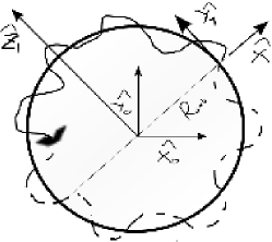
Figure 5: In our proposed $p$-orbits, the orbital distance undergoes a “secondary” oscillation (2nd-Osc) in the way $R=R_{0}+R_{1}\cos(\omega_{1}t)$ (which is simultaneous with an oscillation in the AM (or angular velocity) $\omega$ of the nucleus, vanishing on average). It may look a counterintuitive trajectory for a central potential, but mind the intervention of the “inner” degree of freedom! The frequency matching condition for a $p$-orbital is $\omega_{1}=n_{p}\omega_{0}$. This basic $p$-orbit gives rise to a rotationally invariant electronic density around the axis $\mathbf{z}_{1}$. When we analyze the situation in 3D, we have to consider a modulation of our stabilizing interaction from the misalignment of that axis $\mathbf{z}_{1}$ and the magnetic moment of the electron $\mu_{e}$ (this misalignment is nothing but the classical counterpart of the quantum LS term).

XI.7.2 Stationarity and stability

To proof stationarity, it is enough to show that the system, in absence of rad/abs terms that will further on privilege a discrete set of orbits and explain their attractive behavior, has a frequency description where all poles are purely imaginary. To analyze it, we first had to linearize around a particular point of equilibrium, but once the secondary oscillation dynamics is included, neither of the dynamical variables used in our description of the system (see…) adopt a constant value around the stationary orbit. Anyway, we can keep on considering that the oscillations in $v^{(o)}_{t}$ are small, and the description already used in Sec.IX still remains adequate. The attraction behavior is again provided once we include the rad/abs terms. We would need to prove that this new balance is attainable. We do not consider this a major difficulty, however, and we leave any calculations for the Appendix.

XI.8 Feasible $s$-orbits

In the way that we have done for the $p$-spectrum, we introduce a parameter $n_{s}$, which will later allow us to establish a correspondence with the well known principal quantum number. Initially,

$$R \approx R_{0}\cos(\omega_{0}t),$$ (160)

$$v^{(o)}_{t} \approx v^{(s)}_{t,0}\cos(\omega_{1}t).$$ (161)

XI.8.1 $s$-matching condition

Now we have

$$\omega_{1}=2n_{s}\omega_{0},\quad n_{s}=1,2,\ldots,$$ (162)

yielding

$$R \approx R_{0}\cos(\omega_{0}t),$$ (163)

$$v^{(o)}_{t} \approx v^{(s)}_{t,0}\cos(2n_{s}\omega_{0}),$$ (164)

where, clearly, the higher the $n_{s}$ the higher the energy, and where the amplitude of the 2nd-Osc, this time affecting what we defined as the tangential velocity component, will possibly depend on $n_{s}$, determined by the dynamical equations of the system:

$$v^{(s)}_{t,0}=v^{(s)}_{t,0}(n_{s}),\quad n_{s}=1,2,\ldots,$$ (165)

Special attention should be taken to the factor $2$: we need a trajectory that “crosses ” with itself, so the average AM over a whole cycle yields exactly zero. Again, the reason for the absence of solution $n_{s}=0$ is that it disregards the 2nd-Osc so typical of our system. Following our program, as we did for the p-case, we now have to check if they are indeed stationary, and then if they can be stable (strict stability happens whenever a power balance can be attained, singling out a particular trajectory from the set of all stationary ones).

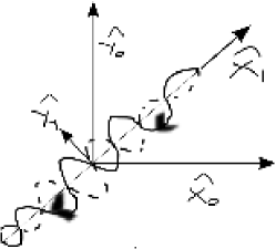
Figure 6: In the proposed $s$-orbits, the secondary oscillation (2nd-Osc) takes place in $\mathbf{y}_{1}$, as well in small variations of the angular momentum (AM) of the nucleus (that vanish, in average). The average overall AM of this orbit is zero as expected for the quantum mechanical counterpart. The frequency matching condition for an $s$-orbital is $\omega_{1}=2n_{s}\omega_{0}$, with $n_{s}=4$ in this example. It may look a counterintuitive trajectory for a central potential, but mind the intervention of the “inner” degree of freedom! Of course this trajectory is not stationary in the purely electrostatic picture, but it is feasible when we include both the Lorentz and higher order terms. On the other hand, this basic $s$-orbit gives rise to a rotationally invariant electronic density in 3D, when the axis $\mathbf{x}_{1}$ is allowed to precess freely in response to stochastic perturbations.

XI.8.2 Stationarity and stability

Our reasoning is the same as for the $p$-spectrum: if we consider that the secondary oscillation (2nd-Osc) is small enough, then the linearized description of the system used in Sec. X remains approximately correct, and the purely imaginary character of the poles in the frequency representation, hence the purely oscillatory behavior, guaranteed. Once the existence of a continuum of stationary orbits is proved for the equations of the system in absence of dissipation/absorption terms, their inclusion privileging a discrete set of orbits (and explaining the attraction behavior).

Our next task will be to do a first approach to the energy spectrum. We have already given the basic equations for the stable orbits (for the linearized system, in 2D and etc.), parameterized them by a natural number $n_{s}$ or $n_{p}$, and now we want to estimate the quantity $\Delta E(n_{\alpha},n_{\alpha}+1)=E(n_{\alpha}+1)-E(n_{\alpha})$. I.e., we want to estimate the energy gap between adjacent states.

XII A first approach to the E-spectrum

In principle, we would have to calculate the following energies, for $p$ and $s$-orbits, respectively,

$$E^{(p)}(n_{p})=E_{1}^{(p)}(n_{p})+E_{2}^{(p)}(n_{p}),$$ (166)

$$E^{(s)}(n_{s})=E_{1}^{(s)}(n_{s})+E_{2}^{(s)}(n_{s}),$$ (167)

where the subscripts $1,2$ make reference to the principal (orbital) or secondary oscillatory movements that characterize each orbit. We will hereon omit superscripts for simplicity (the dependence on $n_{s}$ or $n_{p}$ eliminates any ambiguity).

XII.1 The $p$-spectrum (in absence of 2nd-Osc)

For $p$-orbits, disregarding the 2nd-Osc, we know from (208),

$$E_{1}(n_{p})=-E_{kin}(n_{p})=-\frac{1}{2}m_{e}(v^{(o)}_{r})^{2}=-\frac{1}{2}m_{e}\omega_{0}^{2}R_{0}^{2},$$

and now, applying the frequency matching condition, $\omega_{1}=n_{p}\omega_{0}$,

$$E_{1}(n_{p})=-\frac{1}{2}m_{e}\frac{\omega_{1}^{2}}{n_{p}^{2}}R_{0}^{2},$$ (169)

but, from (229),

$$\omega_{1}\propto\frac{1}{R_{0}^{4}},$$ (170)

so, therefore

$$E_{1}(n_{p})\propto-\frac{1}{n_{p}^{2}}\frac{1}{R_{0}^{2}}.$$ (171)

Considering that

$$\frac{1}{R_{0}^{2}}\approx\frac{1}{R_{0}^{2}}-2\frac{1}{R_{0}^{3}}(R-R_{0})+\ldots,$$ (172)

with $R(n_{p})-R(n_{p}=2)<<R(n_{p}=2)^{3},\ \forall n_{p}>2$, we can make the approximation

$$\frac{1}{R_{0}(n_{p})^{2}}\approx\frac{1}{R_{0}(n_{p}=2)^{2}},\quad n_{p}\geq 2,$$ (173)

and finally arrive to

$$\Delta E_{1}(n_{p},n_{p}+1) = E_{1}(n_{p}+1)-E_{1}(n_{p})$$ (174)

$$\propto \left[\ \frac{1}{n_{p}^{2}}-\frac{1}{(n_{p}+1)^{2}}\ \right],$$

and therefore $\Delta E_{1}(n_{p},n_{p}+1)>0$ as expected.

Doing a finer estimate, however, from Appendix B.3 we can see that actually

$$\frac{1}{R_{0}^{2}} \propto n_{p}^{\frac{4}{5}},\quad\Rightarrow E_{1}(n_{p})\propto-\frac{n_{p}^{\frac{4}{5}}}{n_{p}^{2}}.$$ (175)

but one has to bear in mind that all these estimates are done on a two-dimensional model of the problem, so their significance is only relative.

XII.2 The $s$-spectrum (in absence of 2nd-Osc)

For $s$-orbits, disregarding the 2nd-Osc, we know from (217),

$$E_{1}(n_{s})=-E_{kin}(R=0)=-\frac{1}{2}m_{e}\omega_{0}^{2}R_{0}^{2},$$ (176)

but applying the frequency matching condition, $\omega_{1}=n_{s}\omega_{0}$,

$$E_{1}(n_{p})=\frac{1}{2}m_{e}\frac{\omega_{1}^{2}}{n_{s}^{2}}R_{0}^{2}+E_{pot}(R=0),$$ (177)

but, from (229),

$$\omega_{1}\propto\frac{1}{R_{0}^{3}},$$ (178)

so, therefore

$$E_{1}(n_{s})\propto-\frac{1}{n_{s}^{2}}\frac{1}{R_{0}}.$$ (179)

Considering that

$$\frac{1}{R_{0}}\approx\frac{1}{R_{0}}-\frac{1}{R_{0}^{2}}(R-R_{0})+\ldots,$$ (180)

with $R(n_{s})-R(n_{s}=1)<<R(n_{s}=1)^{2},\ \forall n_{s}>1$, we can make the approximation

$$\frac{1}{R_{0}(n_{s})^{2}}\approx\frac{1}{R_{0}(n_{s}=1)^{2}},\quad n_{p}\geq 1,$$ (181)

and finally arrive to

$$\Delta E_{1}(n_{s},n_{s}+1) = E_{1}(n_{s}+1)-E_{1}(n_{s})$$ (182)

$$\propto \left[\ \frac{1}{n_{s}^{2}}-\frac{1}{(n_{s}+1)^{2}}\ \right].$$

Actually, if we do a finer estimate using the results of Appendix B.3 we can see that actually

$$\frac{1}{R_{0}} \propto n_{s}^{\frac{2}{3}},\quad\Rightarrow E_{1}(n_{s})\propto-\frac{n_{s}^{\frac{2}{3}}}{n_{s}^{2}},$$ (183)

where again we remind the reader that all these estimates are done on a two-dimensional model of the problem, and under many simplifications, so their significance is only relative.

XII.3 2nd-Osc in the E-spectrum?

For the moment, we will not include $E_{2}^{(p)}(n_{p}),E_{2}^{(s)}(n_{s})$ in the calculation. There is a reason for this. Our secondary oscillation (2nd-Osc) expresses a resonance behavior: the system has the capacity of absorbing/dissipating whatever power is necessary to keep its orbital movement at a particular frequency ($\omega_{1}$). Therefore, the energy corresponding to that 2nd-Osc is, always, “immediately” absorbed or given to the background, and with this we mean that in a much smaller time scale than the one corresponding to the principal oscillation (that, from the point of view of this 2nd-Osc, exhibits a practically constant behavior). This is the main reason why we believe this energy should not be included in the estimate of the energy spectrum.

XIII Non circular orbits in 2D: elliptical. Orbits with higher AM

We have so far only addressed the (trivial) case of circular orbits in the plane (2-dimensional problem). Bohr used elliptical orbits to account for states with quantum number $l>1$. This would be the starting point in our approach, as well. More complicated stable orbits (“limit cycles” in the literature of systems theory), given by the nonlinear nature of the dynamical system, require a more sophisticated analysis, but some simple “mind experiment” (giving some initial condition $v_{r}^{(o)}\neq 0$ in the planar problem, for instance) may surely convince the reader that these do actually exist.

Of course, once we have a nonlinear behavior, stability is restricted to certain ranges for initial conditions. This is another task. Comment on the possibility of elliptical attractors. Use of the Poincaré method.

XIV A 3D model

Only some general, preliminary ideas here. Convenient to include it anyway.

XIV.1 A first approach to $p$-orbits in 3D

When we consider general initial conditions, the new forces and/or torques (to the leading order) are strictly normal to the ones in the planar case, so the stability mechanism remains valid. To make our picture consistent, the classical counterpart of the quantum LS interaction must appear here as one of the new terms. This interaction would modulate the strength of our stabilizing mechanism: it decreases its intensity if the magnetic moment $\boldsymbol{\mu}_{e}$ is not aligned with the axis $\mathbf{z}_{1}$ for the circular orbit. On the other hand, we know that a dipoling interaction between magnetic moments of electron and proton must be also present (although it does not appear as a primary term in the Hamiltonian expansion), and it tends to anchor the relative direction of those two moments. The combination of this last dipoling interaction with the classical counterpart of the quantum LS must be the key to determine the probability distribution of some “preliminary” $p$-orbitals in 3D. We say preliminary because we are also considering all the way here that the inner structure of the nucleus is perfectly isotropic: nothing further from truth. Perhaps those differences may well explain the lack of rotational symmetry (not even around the axis of the orbit) of the “real”, quantum, $p$-orbitals.

XIV.2 A first approach to $s$-orbits in 3D

For this kind of trajectories we directly include here some ideas on the extension to 3D. On physical terms, the situation we have is one where the electron oscillates back and forward, moving in a direction that, due to stochastic interaction with the background, can freely precess giving rise to an spherically symmetric set of trajectories. Of course, reorientation of the spin of the electron is needed, but this is the consequence of the terms in Sec. IV.10. This is the kind of behavior we would expect for a quantum s-orbital. Hay que elaborar más la interpretación de cada término en Sec. IV.10.

XV Simulations

Numerical simulations. No simulations for the moment.

XVI The quantum hydrogen: atomic orbitals

We now relate our results to strictly quantum features of the real hydrogen atom. With this section we complete the bridge from our SED context to QM.

XVI.1 Classical and quantum AM

Classical and quantum angular momentum (AM) are often treated as different concepts with only a limited relation between them. If we let aside rotations that are not (globally) isomorphic to the group $SO(3)$ of rotations in ordinary space, the main difference between the concepts of classical and quantum AM is that the former can not in general be added, because of their dependence on the chosen point in respect to which they are evaluated. However, the average value of a classical AM on a closed, periodic trajectory is independent of the origin, as we will see from the following calculation.

Consider an origin of coordinates $\mathbf{O}_{1}$ and let $\mathbf{r}_{1}$ be the position vector defined in respect to it, as well as a second origin of coordinates $\mathbf{O}_{2}$ such that the position vector is now $\mathbf{r}_{2}$. Obviously, the following difference

$$\mathbf{r}_{1,2}=\mathbf{r}_{2}-\mathbf{r}_{1}=\mathbf{O}_{1}-\mathbf{O}_{2},$$ (184)

is clearly a constant vector. Now, let $\Lambda$ be a closed trajectory, with a period $T$, so $\mathbf{r}_{i}(T)=\mathbf{r}_{i}(0)$, for $i=1,2$. For the movement of a system of mass $m$ whose position is (simultaneously) given by $\mathbf{r}_{1}(t)$ and $\mathbf{r}_{2}(t)$, in the respective system of reference, it is easy to prove:

$$\langle\mathbf{L}_{2}\rangle_{\Lambda} = \frac{1}{T}\int_{0}^{T}\mathbf{L}_{2}\ \mathrm{d}t=\frac{1}{T}\int_{0}^{T}\mathbf{r}_{2}\wedge\mathbf{p}\ \mathrm{d}t$$ (185)

$$= \frac{1}{T}\int_{0}^{T}(\ \mathbf{r}_{1}+\mathbf{r}_{1,2}\ )\wedge\mathbf{p}\ \mathrm{d}t$$

$$= \frac{1}{T}\int_{0}^{T}\mathbf{r}_{1}\wedge\mathbf{p}\ \mathrm{d}t+\frac{1}{T}\mathbf{r}_{1,2}\wedge\int_{0}^{T}m\frac{\mathrm{d}\mathbf{r}_{1}}{\mathrm{d}t}\mathrm{d}t$$

$$= \langle\mathbf{L}_{1}\rangle_{\Lambda}+\frac{1}{T}\mathbf{r}_{1,2}\wedge m\left[\ \mathbf{r}_{1}(T)-\mathbf{r}_{1}(0)\ \right]$$

$$= \langle\mathbf{L}_{1}\rangle_{\Lambda},$$

Thus, the classical AM averaged over a closed orbit is independent of the origin and can be added up, just like its quantum counterpart, which suggests a possibility of relating both concepts. For instance, for a $p$-orbit $\Lambda_{p}$, $\langle\mathbf{L}_{1}\rangle_{\Lambda_{p}}=\langle\mathbf{L}_{2}\rangle_{\Lambda_{p}}=\hbar/2$, and for an $s$-orbit $\Lambda_{s}$, $\langle\mathbf{L}_{1}\rangle_{\Lambda_{s}}=\langle\mathbf{L}_{2}\rangle_{\Lambda_{s}}=0$.

XVI.2 On the concept of classical “orbital”

Most of the time, we have been talking about trajectories, rather than orbitals. We feel in need to establish a clearer and more convincing bridge from one concept to the other. We have worked with orbits, or closed trajectories, in the plane. As a matter of fact and keeping an eye on the quantum orbitals, the extension to the 3D problem arises the need to generalize that concept to a new one, that of an “orbital”. We probably said before that with the term “orbital” we mean a collection of points in the configuration space of the system, meeting the condition that, if the system is inside, it would probably stay inside with overwhelming probability. With this concept we are going two steps forward. On one side, where needed we generalize from one particular trajectory to a set of them (for example, a set of s-orbits containing all possible directions, so the resulting orbital exhibits spherical symmetry). On the other, we introduce the stochastic character; those stationary orbits, when subjected to the action of a perturbating background, gives rise to a probability distribution.

Besides, so far we have only been always talking about “orbits” as “closed” or “periodic” trajectories. In regard to this, we must say that “stability” can also be seen as a consequence of a more “chaotic” dynamics, for example through trajectories that adopt the so-called “fractal” kind of behavior: it never goes through the same point (initial condition or state) twice, but the evolution stays forever into some particular region of the configuration space (space of values for the dynamical or state variables) of the system. At this point we have already shown that, at least in an idealized model, this purely classical stable orbitals exist, and they have a discrete character, in the sense that each of them correspond to a particular stationary trajectory (or a set of them). This is indeed the case of our s-orbitals. By contrary, p-orbitals in 2D arise from one particular circular trajectory. Their extension to 3D requires to consider a modulation through the classical counterpart of the quantum LS effect.

XVI.3 Equivalence to quantum orbitals

XVI.3.1 The “node” problem

(to be updated: the LS argument does not work in the $l=0$ case, but we can invoke Fritsche’s reasoning: pure states cannot be prepared)

Ultimately, our classical orbitals are characterized by a probability distribution of the electron around the nucleus. The density of probability may extend to infinite, due to the fact that there is a non-vanishing probability that high values of the background field introduce such strong oscillations in the particle movement (anyway, the bulk of the distribution must be confined to a finite region of space). Therefore, our picture can find quite a consistency with the purely quantum one. Besides, it must be said here that, while non relativistic orbitals in the hydrogen problem show disconnected regions and nodes where the probability density vanishes, this is not the case of the fully relativistic ones (for instance see Szabo69 ).

XVI.3.2 Phase averaging and symmetry

(to be completed)

For both types of stationary orbits, the whole spectrum of stable trajectories we just proposed exhibits several free parameters: the phase (for a given principal axis) in the case of the circular ones, the principal direction in the second case (s-orbits). Now, in both cases, when averaged over all possible angles and phases, they recover the symmetry of the lowest one. Their associated distribution of probability is centered, nevertheless, at a different orbital radius, as the point of balance of radiated and absorbed power is this time different. This is an important step towards the quantum orbitals. Now we recall Figs. 6 and 5. With those in mind we present the following two figures: 7 and 8.

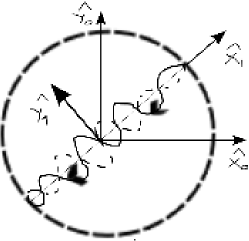
Figure 7: The basic $s$-orbit that gives rise to a rotationally invariant electronic density in 2D, when the axis $\mathbf{x}_{1}$ is allowed to precess freely in response to stochastic perturbations. It may look a counterintuitive trajectory for a central potential, but mind the intervention of the “inner” degree of freedom!

Figure 8: The basic $p$-orbit that gives rise to a rotationally invariant electronic density around the axis $\mathbf{z}_{1}$. When we analyze the situation in 3D, we have to consider a modulation of our stabilizing interaction from the misalignment of that axis $\mathbf{z}_{1}$ and the magnetic moment of the electron $\mu_{e}$ (this misalignment is nothing but the classical counterpart of the quantum LS term).

The extension of the $s$-orbits to 3D had already been discussed before, in Sec. XIV.2. About the $p$-orbitals in 3D, we can only say, for the moment, that clearly we have a trajectory that is associated with a particular direction is space. Whether there may be only three orthogonal directions giving rise to simultaneous stable trajectories is a question that we will left aside for the moment.

XVI.3.3 $n_{s},n_{p}$ against the quantum number $n$

With $n$ the principal quantum number, the correspondence is completely straightforward,

$$n_{p} \rightarrow n,$$ (186)

$$n_{s} \rightarrow n,$$ (187)

with $n_{p}$ and $n_{s}$ as defined in Secs. XI.7 and XI.8. It is remarkable that in our framework, no $n_{s}=0$ or $n_{p}=0$ stationary (hence not stable either) orbits exists, due to the presence in the equations of the 2nd-FL that we have already commented in Sec. VII.2, for instance, and therefore we do not have to exclude that possibility as an “ad hoc” hypothesis. Another question is why should we exclude the $n_{p}=1$ case (the first quantum $p$-orbital corresponds to $n=2$). A closer inspection of the equation for the orbit leads to think that, due to obvious the lack of inversion symmetry when $n_{p}=1$, the implicit decoupling of the movement in an orbital (primary) and secondary oscillations (2nd-Osc) cannot be assumed any more.

XVI.4 Orbital double occupancy: ideas

A flip of the electron spin corresponds to a sign inversion for the classical magnetic moment of the electron, from $\mu_{e}\mathbf{z}$ to $-\mu_{e}\mathbf{z}$. As a consequence, terms corresponding to the Lorentz force and our Inverse Magnitude Spin Orbit (IMSO) coupling reverse sign. This accounts for a shift in the energies (the electrostatic terms obviously remains constant), but in a way that stability remains equally valid, both for the $s$ and $p$-case. In our conclusions we will comment more on this issue, even suggesting an interpretation in terms of a classical Pauli principle, that now arises as a consequence of our model rather than being an “ad-hoc” hypothesis.

XVII Discussion

Here, we try to add clarity on some points. We may also comment on alternative approaches to some of the questions treated so far.

XVII.1 Rad/abs in the dynamical equations

Perhaps we would need to dedicate some more attention to the way in which we include rad/abs in the dynamical equations of the system. This is done in equations (90), (89) and (91), by means of the new terms (86), (83) and (87). Those terms represent an unbalance of radiated and absorbed power in a quasi-instantaneous, but not instantaneous, basis. Therefore, they are averages, but over an interval small enough so that the dynamic included in (90), (89) and (91) stays, effectively, “frozen”.

Looking at (78)–(80), we see the first of them is a cubic polynomial on $\omega_{(o)}$, while the second is a fourth order one (both positively defined for $\omega_{(o)}$ positive). Clearly, this two curves do cross each other, the point where they do so being modified by the extra factor $R_{orb}^{2}$. This obviously gives rise to some “attraction” around a certain value $\omega_{(o)}^{st}$. Above this value, the probability of loss prevails. Below that value, the probability of absorption prevails. We must recall here that, in our formulation, $\omega_{(o)}$ is not one of the state variables of the model, but the tangential velocity component $v^{(o)}_{t}=\omega_{(o)}R_{orb}$, and also $\omega=\omega_{(R)}+\omega_{(o)}$ are so themselves.

We are interested, at least primarily, on circular orbits. Stationarity of these imposes an extra relation on the pair $R_{orb}$, $\omega_{(o)}$, aside from angular momentum (AM) quantization, already obtained from the balance of average power around a closed orbit. This condition results in the corresponding (discrete) set of pairs of values, and therefore, it is justified to employ a prevailing dependence on $R_{orb}$ for $\chi_{r}$, as it is done in (83). This dependence can be linearized around the point of interest. Strictly speaking, we know that Puthoff’s equations (78)–(80) only apply to those circular orbits, but we have extrapolated that behavior to a situation where the system is varying dynamically the parameters of its orbit, and therefore this does not have to remain circular or stable at all (its stability or instability being precisely the ultimate object of our study here). The extrapolation seems natural in the case of (83), anyway.

Less evident is our choice for (86) and (87). For the first of them, we can simply state that because we have, as defined, $v^{(o)}_{t}=\omega_{(o)}R_{orb}$, an attractor in $\omega_{(o)}^{st}$ induces one in $v^{(o)}_{t}|_{st}=\omega_{(o)}^{st}R_{orb}^{st}$. In the case of (87), we have that $\omega=\omega_{(R)}+\omega_{(o)}$ is none other than the angular velocity of rotation of a charge distribution around its axis, always in respect to an inertial frame of reference. Therefore, the rad/abs game applies again, and it is natural to assume that an attractor must exist at a certain value $\omega=\omega|^{st}$. Indeed, we have seen, for the simplest of stationary states, $\omega|^{st}=\omega_{(o)}|^{st}$.

The reader will agree that this is still hardly a rigorous treatment, but we are content to show that stability is not only possible, but arises as a natural behavior purely from the dynamical equations of the system. Though we have made some assumptions, they are rather natural.

XVII.2 Relativistic considerations, “rigidity” and self-reaction forces

Within our context here, all the discussion about the implications of a point particle in electromagnetism is unnecessary. On one hand, and sufficiently away, the electron is seen as a point-like magnetic dipole (which is conventional, again, sufficiently far). On the other, far but not infinitely far, the proton is seen as a distribution of charge (and magnetic momentum) that can “rotate” as a whole. Besides, any reference to the rigidity of the distribution can be regarded as a device to make calculations simpler, but, qualitatively speaking, makes no difference in relation to our main results. As matter of fact, throughout our development in Sec. IV, in no moment we have considered the forces that some elements of charge in the distribution exert over other elements in that same distribution; indeed, the mechanism we expose is dominant up to a certain order, whenever the two objects remain sufficiently apart. Higher orders may deform the shape of the distribution, or have other effects that, whenever the range of distance is the appropriate, do not affect our main argument.

We have nevertheless already briefly commented on the (relativistic) difficulties that arise, not only (i) when we deal with “rigidity”, but also (ii) with the picture of spin as a spinning sphere, rotating around its axis, if we try to adjust the angular velocity so as to reproduce the (phenomenological) magnetic moment of the proton. The difference there is made in what kind of distribution we assume. Simple models such as those of a rotating solid sphere or a spherical shell of charge are ruled out; on the contrary the quark model, where some discrete entities carry charge, and more important to our purposes, all the magnetic momentum, seems to solve those difficulties.

XVIII Conclusions

XVIII.1 General conclusions

In this paper, we have tried to reasonably establish a framework to support the idea that SED (i.e., classical Maxwellian electromagnetism plus a background of radiation), in combination with a model of the nucleus where this presents some very elementary inner structure (specifically, a model of the proton as a spatial distribution of charges), is perfectly capable of explaining atomic stability. Perhaps we should remark, before any other feature of our model, the following point: an atomic transition implies an emission/absorption of a wave-packet with an energy $\hbar(\omega_{i}-\omega_{j})$, where $\omega_{i},\omega_{j}$ are simply the orbital angular frequencies of the basic stable orbits corresponding to the orbitals involved. This comes as a consequence of our very basic hypothesis, rather than being introduced as a principle as it does in QM.

Along with the ideas, we have done many specific calculations that, for the moment, reinforce our previous qualitative approach. They must, nevertheless, be regarded only as preliminary and we hope they will help, on future developments, to check whether we can go forward and converge to more accurate estimates of quantities such as the hydrogen atomic spectra. The ultimate goal of this paper is, therefore, to settle a plausible framework, not necessarily completely quantitative.

XVIII.2 The IMSO coupling

The first main result presented in this paper is the identification of a classical mechanism that appears to be capable of stabilizing the electronic orbitals against (small) perturbations. This mechanism becomes exposed once second order moments are considered for a distribution of charges, under the action of a point-like magnetic source. This interaction couples the magnitude of the angular momenta of the orbital movement, with the magnitude of the inner AM carried by the charge distribution rotating around its axis of symmetry.

In Sec. II.4 we did a quick overview of the main terms in the classical (also quantum mechanical) Hamiltonian for the hydrogen atom. These range, as a result of a multipole expansion for the proton, from (i) the purely Coulomb term, (ii) the Lorentz interaction, (iii) the dipoling (or in QM, spin-spin) interaction, to (iv) the spin-orbit interaction (or LS in QM). That said, if we now include the second order (spatial extension) for the nucleus, we get the terms corresponding to what we have called IMSO coupling. The identification of this higher order interaction is done in two steps. Having worked with a previous electromechanical model, with, in principle, no resemblance with the actual hydrogen atom, we later depart from it and reinterpret our equations in Sec. V. Its presence in a realistic system (a hydrogen atom) is now established.

Another question is why we name it by “spin-orbit”. This is done because, certainly, it bears quite a relation to the conventional spin-orbit coupling (LS term in QM): it is, in order, the following correction to orbital movement of the electron around the nucleus. Nevertheless, we must stress several facts here:

(a) First, we are talking about a coupling between the AM of the electronic orbit and a classical inner AM of the proton (nucleus), not that of the electron. Through more or less complicated arguments, we link this classical AM to a residual oscillation of the proton as a composed object (the quarks inside being point-like entities carrying charge and spin - inner AM), in the form of a rotation around its axis of symmetry. The integral of this oscillation would vanish, so in average the value of the classical (inner) AM would correspond to the quantum mechanical value: from here, our choice of the terms “residual spin” (RS) and “Inverse Magnitude Spin Orbit coupling” (IMSO).

(b) We have to insist in that hey are terms of a different nature. In QM, the LS term couples an effective magnetic field, resulting from the orbital movement of the proton from a reference frame attached to the electron, to the orientation of a magnetic dipole (that of the electron), not changing its magnitude. Our IMSO interaction couples the magnitude of the AM of the orbit (given by the pair of variables $\omega_{(o)}$ and $R_{orb}$) to the magnitude (magnitude of the oscillations) of that “residual spin” of the proton (coming from a non-zero value of $\boldsymbol{\omega}$), not to its orientation, in contrast to what the well-known LS term in quantum atomic physics does (there, the coupled spin is that of the electron).

(c) Probably, the contribution on an average over a closed orbit of this new term is always vanishing (again in contrast to the quantum - or classical - LS shift). A convincing general proof of this is not within our reach yet. On a quasi-instantaneous scale (transparent to QM) this kind of effect would indeed be observable, but at least not by conventional atomic spectrography.

Aside, because our high order interaction takes place exclusively via the Lorentz law, it is reasonable to expect that such correction in the energy spectrum vanishes identically, although this is a matter still to be proven more rigorously. Indeed, we tried to shed some more light on this question with some calculations in Sec. A.1 (Appendix).

XVIII.3 Why is it stabilizing?

Stability of the atomic orbitals is, at least at present, an exclusively quantum mechanical prediction. On the other hand, within the SED framework and up to now, the ZPF background provides a mean to counteract the loss of energy that a charge undergoes when accelerated, through radiation. However, given the stochastic nature of the ZPF, the cancellation is just on average. Nothing, however, had been said yet on how could this balance be attained on a quasi instantaneous basis, or how the orbit could accommodate the instantaneous excess or defect of energy without modifying the pair $R_{orb}$, $\omega_{(o)}$ (therefore keeping the stationarity of the trajectory, losing it otherwise). In other words, it does not explain why the system should remain confined to a reduced portion of its possible configuration space, that portion corresponding to what we know by an orbital.

It does not explain, neither, why there should exist a discrete set of energies for the orbitals with a given AM. However, if we provide the system with the capacity of storing energy on the fluctuations in that classical (residual) “spin” of one of the particles, the former picture can be now made to work. This classical residual spin of the particle must nevertheless be able to participate in an interplay of energy exchange with the orbital degrees of freedom, and in this paper we have shown that the forces and torques for this are present, once that one simply allows for a slightly more complex model of the situation, where the nucleus is permitted to have a non vanishing second order moment.

Now, the instantaneous excess or defect of energy is stored in the proton “residual spin”, so to say, the (residual) AM due to orbital movement of the quarks within the nucleon structure. Adopting the quark model is necessary because the quarks are carriers of net AM and magnetic moment, avoiding that way difficulties with special relativity (those difficulties arise when the more simple model of an spherical distribution of charge is assumed for the electron, and also for the proton).

XVIII.4 Why a discrete spectra?

Puthoff’s work accounted for the necessity of the quantization of AM, but now, the spectrum of parameters for the stable orbits is also discrete, when we impose a condition of “stationarity” over the dynamical equations of the system (Puthoff’s argument did not take them into account). For instance, for a stable circular orbit, the possible values of both orbital radius $R_{orb}$ and the angular velocity $\omega_{(o)}$ are also discrete, aside from the overall AM. This point is of key importance, as the previous picture only accounted for the discretization of the spectrum of AM. But yet, we could go the opposite way. If, in the first place, we impose stationarity what we have is a continuum set of stationary orbits, all of them plausible candidates to be stable, then, as a second step we can demand Puthoff’s power balance, and end up with only one orbit that would have, therefore, perfectly defined values for its main parameters ($R_{orb}$ and the angular velocity $\omega_{(o)}$), as well as for its overall average AM.

Of course, this does not mean that real orbitals are reducible to neat classical orbits in that way: under the bath of radiation, they oscillate around that privileged trajectory or set of trajectories (this is the natural situation when we formulate the three dimensional problem).

XVIII.5 And infinite?

We had explained the discreteness of the spectrum, but this accounts for only one (feasible) stable trajectory for each particular value of AM. The matter of how can we account for an infinite set of stable orbits for each of those values of AM was the following question to be addressed.

So far, we had only addressed the orbital movement of the electron. This movement, that we had called “primary oscillations”, could be stabilized by a feedback loop (primary) relating radial velocity and relative angular velocity in respect to the nucleus. But moreover, the dynamical equations of the system also include another feedback loop, that we had called secondary, relating the radial and tangential components of velocity. This secondary loop introduces an additional oscillation that takes place entwined with the principal, orbital oscillation. Puthoff’s initial calculation only took into account the primary oscillation, therefore yielding a unique point of equilibrium of rad/abs processes. When the presence of the secondary oscillation (2nd-Osc) is taken into account, an infinite set of points of equilibrium becomes possible: the excess or defect of power in the primary oscillation can be exactly canceled by the absorption or dissipation through the secondary movement.

In principle, that infinite set would be continuum, as well, but the inclusion of an additional, and rather obvious from the point of view of the stationarity of the orbit, restriction relating the frequencies of both oscillations. This restriction recovers the discreteness of the spectrum, but now that spectrum includes an infinite number of stable (classical) states, with increasing energies.

XVIII.6 Stable orbits with and without net AM

The second of the main results of this paper consists of a necessary and sufficient proof of the existence of stable orbits, though only applicable, for the moment, to the lowest energy one for two different sets of closed trajectories. By stable we mean an orbit that, under the effect of a (small) perturbation, tends naturally to go back to its initial configuration. Those perturbations would correspond, in this framework, to the instantaneous differences between emitted and absorbed radiation, once a stochastic background is included..

As a first step, in Sec. IX, a rigorous treatment is provided only for the trivial case of circular orbits in the plane, for which we provide a necessary and sufficient condition. These orbits have, nevertheless, non-vanishing AM, and because of this we can presume they do not correspond to the ground state, but to the so-called $p$-orbitals. Another question is that those circular orbits are isotropic (around their axis of symmetry), while real $p$-orbitals are clearly not. This could be due to the fact that our simplistic model of the atomic nucleus assumes its isotropy, whereas the real hydrogen nucleus posses a clear break of isotropy inherent to the quark model. In Sec. X, an additional (infinite) set of stable solutions is provided to account for the whole (discrete) $s$-orbitals spectrum. These trajectories show vanishing (average) angular momentum. The main axis of each of these $s$-trajectories may randomly precess around the nucleus giving rise to the expected spherically symmetric quantum $s$-orbitals.

Particularly in the case of our $s$-orbits, it is convenient to bear in mind that those trajectories are not stable, nor they are stationary, in the simplified problem of a scalar central potential. For them trajectories to be possible, we must add both the action of the Lorentz force on a point particle, as well as our higher order terms arising from the multipole orders we include in the calculation (our “stabilizing mechanism”). The identification of that last set of stable trajectories with vanishing AM, a set of “candidates” for the s-orbitals, is maybe one of the most important contributions in our present work. Indeed, to our knowledge, it is something not present in any previous treatment on the subject (and of course not in the Bohr model!).

XVIII.7 Equivalence with QM orbitals

Beyond the fact that this SED picture may give rise to stable orbits for the hydrogen atom, the equivalence with the well-known quantum orbitals has been established in the following ways:

(i) Average angular momentum (AM) over the orbit: we have shown the existence of stable orbits whose average AM either vanishes (for the $s$-orbits) or not (for our $p$-orbits). See Secs. X, IX and XI.

(ii) Symmetry properties: as seen in Sec. XVI.3, once phase averaging is done, rotational symmetry is recovered, three dimensional for the $s$-case and around an axis for the $p$-cases..

(iii) Parametrization of the discrete spectrum by a counterpart of the principal quantum number, obtained from an additional frequency matching condition. See Secs. XI.6, XI.8.1 and XI.7.1.

XVIII.8 Energy spectrum

A remarkable approximation to the typical $1/n^{2}$, at least when we include only the principal oscillation, is also obtained. See Secs. XII and the Appendix, Sec. B.5. It is, anyway, a very preliminary result, given that the quantitative analysis is reduced to two dimensions, an isotropic model for the structure of the proton (very far from a realistic one) and the lack of a rigorous approach to the inclusion of the stochastic background. Some of these convenient extensions are discussed briefly in Sec. XIX.

XVIII.9 A possible relation with Pauli statistics?

This is an incidental question, but not devoid of interest at all. Basically, in our framework, stable orbits correspond to modes of oscillation. That correspondence is one to one, which suggest an interpretation in terms of a sort of “classical” Pauli principle.

There is a very interesting interpretation of our results here. Stability of an orbit (or the orbital generated from it) requires vibration of the nucleus in a certain mode. The presence of one of these modes can exclude (or not) the existence of more instances of the same mode, giving rise to a sort of Pauli principle that nevertheless we will only suggest here. For example, for the $s$-case everything seems to suggest that the only possible configuration for two electrons is the one in which their spins are anti-aligned, and that no third one can be included in the stable picture, for a given value of our principal number $n_{s}$. The question would require, as said before, further attention.

XVIII.10 Extension to 3D

A great deal of our conclusions are immediately generalizable to 3D. For instance, we have justified three dimensional rotational symmetry from our proposed stable $s$-orbits. However, in general, extension to the 3D problem requires some extra calculations that for the moment we have not faced here. In particular, the effects of the mechanism we expose here are clearly modulated by the classical counterpart of the LS interaction in QM, between the electron and the nucleus, when the system is allowed to evolve in 3D.

XVIII.11 Additional conclusions

With the aim of shedding some more light on our work, in Sec. XVII we have discussed the approach we adopted to include, in the dynamic equations of the system, the effect of rad/abs as a result of the interaction with the stochastic background. Certainly, our approach is not the most rigorous one, although it is enough so as to show how the equations can lead naturally to a set of privileged trajectories or attractors.

Of course, all this only constitutes a preliminary effort, and more detailed calculations about the specific predicted parameters of those stable orbits (or orbitals, in a wider sense) are awaiting to be done. Moreover, even for the case of elliptical orbits, a strict proof of stability is still lacking. The necessary elements are there, though, and at least in this particularly point, further work is ongoing and will be presented elsewhere. A point that is convenient to stress is that our mechanism belongs to a “simplest one” class. Therefore, calculations based exclusively on our picture here do not guarantee for reasonable estimates, for instance of the $s$ or $p$ energy spectra. Nothing forbids, nevertheless, that further refinements of the model could adjust more to the experimental results. We have seen, already, that special relativity arises the need to assume a “discrete” charge (and magnetic moment) distribution for the proton, and space for much more sophistication is clearly still open in this issue.

As a last remark, David Regalado, student, has performed some calculations on the mean speed of the electron in our proposed $s$-orbitals that agree quite well with the accepted values for the quantum case. This calculations will be presented elsewhere.

XIX On future developments

The main problem that will occupy our time in the next future will consist of trying to extract, in a more rigorous way than what we have done, the well known $\tfrac{1}{n^{2}}$ dependent-spectrum from our framework. In this regard, the calculations presented here can only be considered as very preliminary estimates.

For the moment, what we have proven is that the existence of an infinite, discrete, spectrum is the natural consequence of our model, and we have even done some estimates that bear some resemblance with the real quantities. In any case, from here several main problems are to be addressed, each of them will presumably further correct that first estimate:

(I) The extension of the model to 3D, that we have already treated tangentially in some sections.

(II) The inclusion of anisotropies in the model: mainly, the evident anisotropy in the structure of the proton, and its lack of inversion symmetry. This correction should make our classical orbits (or sets of them, in the three dimensions, and their associated probability distribution once background noise is included) look more like the actual quantum orbitals.

(III) On the other hand, we have not so far predicted any specifical probability distributions, which would in the last term define an “orbital”. Indeed, a very interesting extension of that work would be to predict the density of probability that we would find considering a “broad band” (high frequency-cutoff) model for the fluctuations. Up to now, we have used a “low band” model where the value of the ZPF was averaged over an interval (we did this through the inclusion of the $\chi$-functions, see Sec. VI.2), small enough not to mask the dynamics of the system as an electromechanical mechanism, so we could calculate the “privileged” trajectories or attractors.

Appendix A Additional calc. on the IMSO

We include here several additional calculations, regarding our idealized situation, with no necessary mention to the actual hydrogen atom. Therefore, notation here is in coherence with that of the first part of the paper: we always use $R_{orb}$ and $\omega_{(o)}$ because they are more general and perfectly defined variables (in contrast to $R_{0},\omega_{0},\ldots$, which have different meaning for $s$ or $p$-orbits).

Though not relevant enough to be included in the main body of the paper, they may be useful, however, to interpret further results.

A.1 E-correction for $p$-orbits

The aim of this section was to do a preliminary exploration: it seems, up to now, that the high order terms under our focus do not produce any correction… on average over a whole circular (closed) orbit. This seems reasonable as all the new terms stem from the Lorentz force, for which “work” always vanishes (it is normal to velocity). This question should be treated more carefully in future versions of the paper.

We want to evaluate what shifts in energy are introduced by our IMSO coupling. It is important to state again here that this new correction is of a completely different nature from the well known quantum LS. We have a coupling between (oscillating) magnitudes of classical angular momenta, not just the one between their relative orientations in space.

This said, we will confront the fact that (in some ways “as expected”), our correction vanishes over a whole cyclic orbit. This is a natural consequence of our calculations. Nevertheless, it would be interesting to think how this could be reformulated in terms of work, taking into account the special nature of the Lorentz forces.

Specifically, we insist on the fact that a moving charge in an electrostatic field will “see” a magnetic field, due to Lorentz covariance. This magnetic field produces a force that couples to the charge. In a purely classical picture, we have seen we need to go up to a second order moment to be able to couple this field to the AM with which that charge is rotating around its axis of symmetry.

We have, therefore, a classical coupling between the magnitude of the orbital angular momentum and of what we have called, with the aim of accommodating our reasoning to a physical situation that could resemble a realistic hydrogen atom, “residual spin”. Hence, after all what we have is a new correction term to the classical Hamiltonian (in the same way that one adds new terms to the quantum one). We focus now only on this new energy correction.

On the other hand, and based on the formal equivalence of the equations exposed in Sec. V.2, we can consider that the following calculations are valid for either of the treated situations, the first one comprising two systems of charges, a heavy pointlike one and a lighter extended one, the second being a first model of the hydrogen atom.

As a first approach to characterize quantitatively this new energy correction, we begin by equating, classically, the (radial) force with the centrifugal term. We will first focus on the order of the correction (then more detailed conclusions can be obtained by using the electron, proton mass, charge, magnetic moment, etc).

For a perfectly circular orbit, we have, from (72) with $\dot{v}^{(o)}_{r}=0$ and the perfect compensation (as an expectation value) of radiative loss and background pressure,

$$F_{e}+F_{m}^{(o)}+F_{m}^{(R)}=m\ \frac{(v^{(o)}_{t})^{2}}{R_{orb}},$$ (188)

The terms $F_{e}$ and $F_{m}^{(o)}$ are already present at any classical treatment of the hydrogen atom, and represent, respectively, the electrostatic and the Lorentz (reciprocal, comment on this!) forces. The terms that give rise to $F_{m}^{(R)}$ are the interesting ones.

A.1.1 Kinetic E-correction

The kinetic energy $T=\frac{1}{2}\ m\ (v^{(o)}_{t})^{2}$, and we can compute each correction by:

$$\Delta(T)_{i}\approx\frac{R_{orb}}{2}\ F_{i},$$ (189)

Specifically:

$$F_{e}\propto R_{orb}^{-2}\ \Rightarrow \Delta T_{e}\propto R_{orb}^{-1},$$ (190)

$$F_{m}^{(o)}\propto qB_{1}\ v^{(o)}_{t}\propto R_{orb}^{-2}\ \Rightarrow \Delta T_{m}^{(o)}\propto R_{orb}^{-1},$$ (191)

$$F_{m}^{(R)}\propto\frac{3Q_{2}\omega}{R_{orb}^{4}}\propto R_{orb}^{-4}\ \Rightarrow \Delta T_{m}^{(R)}\propto R_{orb}^{-3},$$ (192)

where we use the sign $\Delta$ all the time because a complete evaluation of the kinetic energy would have to include the term in $\omega^{2}$. From the perturbative point of view, we are only interested in the former ones.

A.1.2 Potential E-correction

We need to compute $\Delta R_{orb}$ as a result of $F_{m}^{(R)}$, and then do, to first order,

$$\Delta V\ \propto\ \frac{1}{R_{orb}}-\frac{1}{R_{orb}+\Delta R_{orb}}.$$ (193)

This accounts for solving a polynomial equation. We multiply by $R_{orb}\ \ +\ \Delta R_{orb}$ on the right,

$$(R_{orb}\ \ +\ \Delta R_{orb})\ \Delta V\ \propto \ \frac{\Delta R_{orb}}{R_{orb}},$$ (194)

$$(R_{orb}^{2}\ +\ R_{orb}\ \cdot\Delta R_{orb})\ \Delta V\ \propto \ \Delta R_{orb},$$ (195)

and therefore

$$\Delta V\ \propto\ \Delta R_{orb}\ \cdot R_{orb}^{-2},$$ (196)

but we also had, from (192), $\Delta T_{m}^{(R)}\propto R_{orb}^{-3}$. Now, in first order to perturbation (we consider the other terms of the kinetic energy $T_{e}$ and $T_{m}^{(o)}$ remain fixed), again selecting the leading terms,

$$\Delta T_{m}^{(R)} \propto \frac{1}{2}m\ \omega_{orb}^{2}\ \left[\ (R_{orb}+\Delta R_{orb})^{2}-R_{orb}^{2}\ \right]$$ (197)

$$\propto \frac{1}{2}m\ \omega_{orb}^{2}\ \left[\ 2R_{orb}\Delta R_{orb}\ \right]$$

$$\propto m\ \omega_{(o)}^{2}\ R_{orb}\ \Delta R_{orb},$$

and therefore,

$$\Delta R_{orb}\propto R_{orb}^{-4},$$ (198)

so we can neglect the correction to the potential energy $\Delta V\propto R_{orb}^{-6}$.

A.1.3 Order of the full correction

Our first idea was to compare our estimate with the value of $\langle\psi_{GS}|\ L\cdot S\ |\psi_{GS}\rangle$, the first correction in the perturbation expansion of the energy predicted by non-relativistic QM for the ground state $|\psi_{GS}\rangle$ of the system. Now, from Sakurai_ad (page 88), we have, for a central potential, the leading term with $L\cdot S$ has the magnitude

$$\frac{1}{mc^{2}}\cdot\frac{1}{r}\cdot\frac{dV}{dr}\propto R_{orb}^{-3},\ \ \ r=R_{orb},\ \ \ V\propto R_{orb}^{-1},$$

for a Coulombian potential. It does agree, therefore, with the order of our leading correction $\Delta T_{m}^{(R)}$ (!) in (192). Nevertheless, we must stress our correction is of a completely different nature, coupling oscillations on the magnitude of a classical AM vector, not on its orientation as the quantum LS does (see Sec. II.4).

Then, what is the interest of this comparison? In nuclear physics, phenomenological (ad hoc) terms with the LS form are introduced in order to explain the negative binding energies (therefore, the stability) of most nuclei. This is a very interesting question that we should treat elsewhere.

There was, anyway, a triviality waiting to be acknowledged here: for a perfectly circular orbit, we simply have $\Delta T_{m}^{(R)}=0$. But still we were interested in that calculation, due to, for an elliptical orbit, it still remains valid in the points where the radial velocity vanishes. In the rest of the points, our correction to the kinetic energy needs to include the velocity component in the radial direction, $v^{(o)}_{r}$ From (72) we have

$$|\dot{v}^{(o)}_{r}|\propto R_{orb}^{-4}\ \Rightarrow \ |v^{(o)}_{r}|=\int{|\dot{v}^{(o)}_{r}|\ dt}\propto R_{orb}^{-4}$$

$$\Rightarrow \ \Delta T\propto|v^{(o)}_{r}|^{2}\propto R_{orb}^{-8},$$

so therefore we can neglect that contribution and simply extend our former analysis to any possible orbit (we have only strictly proved the existence of circular ones).

All this analysis justifies us to stick just to the leading term, and give a complete estimate, using (37):

$$\Delta T_{m}^{(R)} = \frac{R_{orb}}{2}\ F_{m}^{(R)}$$ (201)

$$= \frac{3\hat{\mu}Q_{2}}{2\ R_{orb}^{3}}\ \omega_{(R)}$$

$$= \frac{3\hat{\mu}Q_{2}}{2\ R_{orb}^{3}}\ \left[\ \omega-\omega_{(o)}\ \right],$$

where in the last line we have used (8). To compute the correction, we would average the quantity $\Delta T_{m}^{(R)}$ on all the points of the orbit. We do not tackle this calculation because we have not yet found those stable elliptical orbits.

Appendix B Additional calculations on the H-model

Here we provide additional calculations on the model, once this is completely particularized to account for the hydrogen properties. Whenever the results here are used in the body of the paper, it is always properly referenced. Notation here corresponds to that of the last part of the paper: for convenience, and because there is no possible ambiguity, we use $R_{0},\omega_{0},R_{1},\omega_{1}$ instead of $R_{0}^{(s)},R_{0}^{(p)},\ldots$.

B.1 Energies without 2nd-Osc

B.1.1 Energy of a stationary $p$-orbit

A circular stationary trajectory $\Lambda_{p}$ is given by the pair of parameters $\omega_{0}\equiv\omega_{(o)}$ and $R_{0}\equiv R_{orb}$. Assuming $v^{(o)}_{r}=0$, we can accept the following expression, from (204),

$$R_{0}^{3}=\frac{q^{2}}{4\pi\epsilon_{0}}\cdot\frac{1}{m_{e}\omega_{0}^{2}},$$ (202)

and therefore

$$R_{0}\propto(\omega_{0})^{-\frac{2}{3}},$$ (203)

which means that, in general, if $\omega_{0}$ decreases, $R_{0}$ will increase, which is intuitive for a higher energy orbit. After the inclusion of the secondary oscillation the situation will be, however, slightly more subtle than that, with $R_{0}$ keeping an almost constant (and perhaps even decreasing) value, that nevertheless will not be associated with a decrease in energy. Now, for a circular stationary orbit, $v^{(o)}_{t}=\omega_{(o)}R_{0}$, and we have

$$m_{e}\frac{(v^{(o)}_{t})^{2}}{R_{0}}=m_{e}\omega_{0}^{2}R_{0}=\frac{q^{2}}{4\pi\epsilon_{0}R_{0}^{2}},$$ (204)

and, therefore, in terms of energy,

$$E_{kin} = \frac{1}{2}m_{e}(v^{(o)}_{t})^{2}$$ (205)

$$= \frac{1}{2}m_{e}\omega_{(o)}^{2}R_{0}^{2}$$

$$= \frac{1}{2}\frac{q^{2}}{4\pi\epsilon_{0}R_{0}}$$

$$= \frac{1}{2}qV(R_{0})=-\frac{1}{2}E_{pot},$$

with $V(R_{orb})$ the potential created by a charge with value $q>0$ at $\mathbf{r}_{0}=0$ ($\mathbf{r}_{1}=-R_{orb}\mathbf{x}_{1}$), and therefore, with,

$$E = E_{kin}+E_{pot}$$ (206)

$$= -\frac{1}{2}E_{pot}+E_{pot}=\frac{1}{2}E_{pot},$$

where both $E_{kin}$ and $E_{pot}$ stay constant along the orbit. On the other hand, we can also reverse (205), obtaining

$$E_{pot}=-2E_{kin},$$ (207)

and finally,

$$E = -E_{kin},$$ (208)

$$\Delta E = -\Delta E_{kin}=\frac{1}{2}E_{pot}.$$ (209)

B.1.2 Energy of a stationary $s$-orbit

On the other hand, an $s$-type trajectory $\Lambda_{s}$ is for instance determined by the pair of parameters $v_{max}=\max_{\Lambda_{s}}v^{(o)}_{r}$ and $R_{max}=\max_{\Lambda_{s}}R_{orb}\equiv R_{0}$ (this last equivalence only under the approximation of harmonic dynamics both in the radial and tangential directions). Now, we can equate kinetic and potential energies (for this second one we adopt a convenient absolute reference so it vanishes when it is minimum) at the extremal points (when the velocity is maximum and when it is zero):

$$E_{kin}(R=0)+E_{pot}(R=0)=E_{pot}(R=R_{0}),$$ (210)

and (with $I_{z}$ the $z$-moment of inertia of the nucleus),

$$E_{kin}(R=0) = \frac{1}{2}m_{e}(\omega_{0}R_{0})^{2}+\frac{1}{2}I_{z}\omega^{2},$$ (211)

and

$$E_{pot}(R=R_{0}) = -qV(R=R_{0})-E_{pot}(R=0)$$

$$= -\frac{q^{2}}{4\pi\epsilon_{0}R_{0}}-E_{pot}(R=0),$$

and finally,

$$E_{pot}(R=R_{0})=E_{kin}(R=0)+E_{pot}(R=0),$$

(213)

$$E_{kin}(R=0)=E_{pot}(R=R_{0})-E_{pot}(R=0),$$

but now, disregarding the contribution to the kinetic energy coming from $\omega$,

$$\frac{1}{2}m_{e}(\omega_{0}R_{0})^{2}=\frac{q^{2}}{4\pi\epsilon_{0}R_{0}},\\$$ (215)

and indeed, if no other contribution to the energy is considered (no oscillation in $v^{(o)}_{t}$ or $\omega$ are present), the average energy is

$$E_{kin}(R=0) = -E_{pot}(R=R_{0}),$$ (216)

$$E = -E_{kin}(R=0),$$ (217)

$$\Delta E = -\Delta E_{kin}=\frac{1}{2}E_{pot}.$$ (218)

Of course, the former calculation must assume that the potential energy is bound in the origin $\mathbf{r}_{0}=0$, somehow. This is however compatible with one of the main ideas behind this paper: the introduction of the inner structure of the nucleus in the atomic model. If we adopt now the harmonic oscillator approximation, with $R=R_{0}\cos(\omega_{0}t)$ (where from $\omega_{0}$ does not stand for a rotation in respect to $RF_{0}$ but can still be defined as an angular frequency), then $v_{r}|_{max}=R_{0}\omega_{0}$. Also working with (215),

$$\frac{1}{2}m_{e}(\omega_{0}R_{0})^{2} = -\frac{q^{2}}{4\pi\epsilon_{0}R_{0}},$$ (219)

$$R_{0}^{3} = \frac{q^{2}}{2\pi\epsilon_{0}m_{e}\omega_{0}^{2}},$$ (220)

and again to arrive at a similar condition as in the circular case, this time for the parameter $R_{0}$,

$$R_{0}^{2}\propto(\omega_{0})^{-\frac{1}{3}}.$$ (221)

B.1.3 Potential E-gap between adjacent orbits

We recall once more that, either for the $p$ or $s$ case, and with no rad/abs, our model admits an infinite set of stable trajectories, therefore an infinite set of pairs $\omega_{(o)},R_{orb}$ and $v_{max},R_{max}$. That continuous set will be reduced to a discrete one by means of the imposition of that balance. Let us now consider (feasible) excited states. The main idea here is that, either for the $s$ or $p$ cases,

$$\Delta E\propto\Delta E_{pot},$$ (222)

and moreover, if $R_{orb}$ ($R_{max}$) increases, $\Delta E>0$ because $\Delta E_{pot}>0$ as $E_{pot}<0$.

See where we are going? The same spectrum for $s$ and $p$-type trajectories demands $R_{orb}\neq R_{max}$ for a given value of the principal quantum number $n$, but this is no problem. Let us, for the moment, just work with a generic parameter $R_{n}$ (corresponding to an excited state with quantum number $n$). It is interesting to quantify this increment between the trajectories $n$ and $n+1$ as

$$\Delta E\propto\Delta E_{pot}=\frac{q^{2}}{4\pi\epsilon_{0}}\left[\frac{1}{R_{n+1}}-\frac{1}{R_{n}}\right].$$ (223)

B.2 Determining the parameters of 2nd-Osc

(correction: we write here $\hat{\mu}$ instead of $\hat{\mu}_{e}$… there are some missing factors here)

Aside from the harmonic oscillator approximation, we neglect the change in the electrostatic and Lorentz parts of the potential as a result of the change in the radial coordinate $R=|R_{orb}|$. Those electrostatic and Lorentz terms contribute to the mean centripetal acceleration, but nothing else, at least under our approximation. Therefore, only the term corresponding to our high order model enters in the following calculations.

B.2.1 2nd-Osc for $p$-orbits

For circular orbits, the equations of interest are (72) and (74). Considering that, as already stated, the secondary oscillation (2nd-Osc) can be expressed assuming the radial direction as $\Delta R=R-R_{0}=R_{1}\cos{\omega_{1}t}$, this oscillation univocally determines an associated one for $\omega_{R}\equiv\omega_{(R)}$ (see footnote defs_omega ):

$$\omega_{R}=-\omega_{0}+\omega_{R,0}\cos(\omega_{1}t),$$ (224)

where $\omega_{R,0}$ is determined from $\omega_{0},R_{0}\omega_{1},R_{1}$. Now, we can apply the following two conditions, evaluating the point of maximum acceleration, measured as a variation of the radial velocity (we are already eliminating the centripetal contribution, associated to $\omega_{0}$ in the former expression):

$$\left[\ m_{e}\dot{v}^{(o)}_{r}\ \right]_{max} = \left[\ \frac{3\hat{\mu}Q_{2}}{R_{0}^{4}}\ \omega_{(R)}\right]_{max}\Rightarrow$$

$$m_{e}R_{1}\omega_{1}^{2} = \frac{3\hat{\mu}Q_{2}}{R_{0}^{4}}\ \omega_{R,0},$$ (225)

and

$$\left[\ M_{2}\ \dot{\omega_{(R)}}\ \right]_{max} = \left[\ \frac{3\hat{\mu}\ Q_{2}^{(*)}}{R_{0}^{4}}\ v^{(o)}_{r}\ \right]_{max}\Rightarrow$$

$$M_{2}\omega_{R,0}\omega_{1} = \frac{3\hat{\mu}\ Q_{2}^{(*)}}{R_{0}^{4}}\ R_{1}\omega_{1},$$ (226)

$$M_{2}\omega_{R,0} = \frac{3\hat{\mu}\ Q_{2}^{(*)}}{R_{0}^{4}}\ R_{1},$$ (227)

naturally with $v^{(o)}_{r}|_{max}=R_{1}\omega_{1}$. The two former equations allow us to eliminate $\omega_{R,0}$ and produce a relation between $R_{1}$ and $\omega_{1}$, which is what we were looking for:

$$\omega_{1}^{2} = \frac{3\hat{\mu}Q_{2}}{m_{e}R_{0}^{4}}\ \omega_{R,0}=\frac{9\hat{\mu}^{2}Q_{2}Q_{2}^{(*)}}{M_{2}R_{0}^{8}},$$ (228)

$$\omega_{1} = \frac{3\hat{\mu}\sqrt{Q_{2}Q_{2}^{(*)}/m_{e}M_{2}}}{R_{0}^{4}}.$$ (229)

B.2.2 2nd-Osc for $s$-orbits

For circular orbits, the equations of interest are (72) and (73). Considering that, as already stated, the secondary oscillation can be expressed for the tangential direction as $\mathbf{R}_{orb}\cdot\mathbf{y}_{1}=R_{1}\cos{\omega_{1}t}$. As it already happened for circular orbit, this oscillation univocally determines another one, in this case associated with $v^{(o)}_{r}$:

$$v^{(o)}_{r} = \omega_{0}R_{o}\cos(\omega_{0}t)+\Delta v^{(o)}_{r},$$ (230)

$$\Delta v^{(o)}_{r} = \Delta v_{r,0}\cos(\omega_{1}t),$$ (231)

where $\Delta v_{r,0}$ is determined from $\omega_{1},R_{1}$.

Now, we can apply the following two conditions, evaluating the point of maximum acceleration, measured as a variation of the radial velocity (again we are already eliminating the main, centripetal contribution):

$$\left[\ m_{e}\dot{v}^{(o)}_{t}\ \right]_{max} = \left[\ qB_{1}\ \Delta v^{(o)}_{r}\right]_{max}\Rightarrow$$

$$m_{e}R_{1}\omega_{1}^{2} = qB_{1}\ \Delta v_{r,0},$$ (232)

and

$$\left[\ \Delta(m\dot{v}^{(o)}_{r})\ \right]_{max} = \left[\ qB_{1}\ v^{(o)}_{t}\ \right]_{max}\Rightarrow$$

$$m_{e}\omega_{1}\Delta v_{r,0} = qB_{1}\ R_{1}\omega_{1},$$ (233)

$$m_{e}\Delta v_{r,0} = qB_{1}\ R_{1}.$$ (234)

Now, the two equations allow us to eliminate $\Delta v_{r,0}$ and produce a relation between $R_{1}$ and $\omega_{1}$, which is what we were looking for,

$$\omega_{1}^{2} = \frac{qB_{1}}{m}\ \omega_{R,0}=\frac{q^{2}B_{1}^{2}}{m^{2}}=\frac{q^{2}\hat{\mu}^{2}}{R_{0}^{6}},$$ (235)

$$\omega_{1} = \frac{q\hat{\mu}}{R_{0}^{3}}.$$ (236)

B.3 Approach to the orbital radius spectrum

B.3.1 $p$-orbits

We know

$$m_{e}\omega_{0}^{2}R_{0} = \frac{q^{2}}{4\pi\epsilon_{0}R_{0}^{2}},$$

$$\omega_{1} = \frac{3\hat{\mu}\sqrt{Q_{2}^{(*)}/m_{e}}}{{R_{0}}^{4}},$$

$$\omega_{0} = \frac{1}{n_{p}}\omega_{1},$$

and using (229) as well as our external (it is a supplementary assumption) “matching condition” $\omega_{0}=\frac{1}{n_{p}}\omega_{1}$,

$$\left[\ \frac{1}{n_{p}}\frac{3\hat{\mu}\sqrt{Q_{2}^{(*)}/m_{e}}}{R_{0}^{4}}\ \right]^{2}R_{0}=\frac{q^{2}}{4\pi\epsilon_{0}R_{0}^{2}},$$ (238)

$$\frac{q^{2}}{4\pi\epsilon_{0}}R_{0}^{5}=\left[\ \frac{1}{n_{p}}3\hat{\mu}\sqrt{Q_{2}^{(*)}}\ \right]^{2},$$ (239)

$$R_{0}^{5}=\frac{4\pi\epsilon_{0}}{q^{2}}\left[\ \frac{1}{n_{p}}3\hat{\mu}\sqrt{Q_{2}^{(*)}}\ \right]^{2},$$ (240)

so therefore

$$R_{0}^{5}\propto\frac{1}{n_{p}^{2}},\quad R_{0}\propto\frac{1}{n_{p}^{\frac{2}{5}}},\quad\frac{1}{R_{0}}\propto n_{p}^{\frac{2}{5}},\quad\frac{1}{R_{0}^{2}}\propto n_{p}^{\frac{4}{5}},$$

and so

$$\omega_{0}\propto\frac{1}{R_{0}^{3}}\propto n_{p}^{\frac{6}{5}}.$$ (242)

B.3.2 $s$-orbits

Under the harmonic oscillator approximation, the spectrum of the pendulum orbit maximum radius follows the same rule as for circular orbits. Indeed, from the stationarity equation, where we disregard higher order terms:

$$m_{e}\omega_{0}^{2}R_{0}=\frac{q^{2}}{4\pi\epsilon_{0}R_{0}^{2}},\quad\omega_{1}=\frac{q\hat{\mu}}{{R_{0}}^{3}},\quad\omega_{0}=\frac{1}{2n_{p}}\omega_{1},$$

and using (229) and the matching condition $\omega_{0}=\frac{1}{n_{p}}\omega_{1}$,

$$\left[\ \frac{1}{2n_{p}}\frac{q\hat{\mu}}{{R_{0}}^{3}}\ \right]^{2}R_{0} = \frac{q^{2}}{4\pi\epsilon_{0}R_{0}^{2}},$$ (244)

$$R_{0}^{3} = \ldots,$$ (245)

and so

$$R_{0}^{3}\propto\frac{1}{n_{p}^{2}},\quad R_{0}^{2}\propto\frac{1}{n_{p}^{\frac{4}{3}}},\quad R_{0}\propto\frac{1}{n_{p}^{\frac{2}{3}}},\quad\frac{1}{R_{0}}\propto n_{p}^{\frac{2}{3}},$$

and therefore

$$\omega_{0}\propto\frac{1}{R_{0}^{3}}\propto n_{p}^{2}.$$ (247)

B.3.3 Comments

It is surprising that $R_{0}$ is actually a decreasing function of $n_{p},n_{s}$. Nevertheless, what we do here is simply provide a feasible stable orbit, from which a realistic probability distribution (extended, in principle, to the whole space) could be generated once the stochastic background is included in the picture. Actually, the inner regions or the quantum $s$ and $p$-orbitals do tend to decrease! Besides, in a real atom repulsion between electrons can well explain that the actual mean distances in the orbitals increase with the principal quantum number.

B.4 Modified power balance

So far, we have seen that given $R_{0}$, $\omega_{0}$ and $\omega_{1}$ are determined (the second through our “matching” condition). Therefore, the only free parameter is $R_{1}$. Imposing the radiated/absrobed power balance will fix it.

B.4.1 $p$-orbits: first approach

Firs, we notice that (78) and (80) provided instant averages, rather than averages over the whole orbit, which is important to bear in mind for the following calculation (otherwise, due to $\omega_{0}<\omega_{1}$, some extra factors would be necessary). Now, recovering (78) and (80), we have,

$$\langle P_{rad}\rangle = \frac{q^{2}\omega_{0}^{4}R_{0}^{2}}{6\pi\epsilon_{0}c^{3}}+\frac{q^{2}\omega_{1}^{4}R_{1}^{2}}{12\pi\epsilon_{0}c^{3}},$$

$$= \frac{q^{2}}{12\pi\epsilon_{0}c^{3}}\left[2\omega_{0}^{4}R_{0}^{2}+R_{1}\omega_{1}^{4}R_{1}^{2}\right],$$

as well as

$$\langle P_{ab}\rangle = \frac{q^{2}\hbar\omega_{0}^{3}}{6\pi\epsilon_{0}m_{e}c^{3}}+\frac{q^{2}\hbar\omega_{1}^{3}}{12\pi\epsilon_{0}m_{e}c^{3}},$$

$$= \frac{q^{2}\hbar}{12\pi\epsilon_{0}m_{e}c^{3}}\left[\omega_{0}^{3}+\omega_{1}^{3}\right].$$

Now, applying $P_{rad}=P_{ab}$ and $\omega_{1}=n_{p}\omega_{0}$,

$$2\omega_{0}^{4}R_{0}^{2}+\omega_{1}^{4}R_{1}^{2} = \frac{\hbar}{m_{e}}\cdot\left[2\omega_{0}^{3}+\omega_{1}^{3}\right],$$ (250)

$$2\omega_{0}^{4}R_{0}^{2}+n_{p}^{4}\omega_{0}^{4}R_{1}^{2} = \frac{\hbar}{m_{e}}\cdot\left[2\omega_{0}^{3}+n_{p}^{3}\omega_{0}^{3}\right],$$ (251)

$$2\omega_{0}R_{0}^{2}+n_{p}^{4}\omega_{0}R_{1}^{2} = \frac{\hbar}{m_{e}}\cdot\left[2+n_{p}^{3}\right],$$ (252)

and

$$R_{1}^{2}=\frac{1}{n_{p}^{4}\omega_{0}}\left[\ \frac{\hbar}{m_{e}}\cdot(\ 2+n_{p}^{3}\ )-2\omega_{0}R_{0}^{2}\ \right],$$ (253)

and now we can do a preliminary calculation regarding only the highest order terms, and in the limit where $n_{p}\rightarrow\infty$, taking into account that $R_{0}^{2}\propto\frac{1}{n_{p}^{4/5}}$,

$$R_{1}^{2} \rightarrow \frac{1}{n_{p}^{4}\omega_{0}}\left[\frac{\hbar}{m_{e}}n_{p}^{3}+2\omega_{0}R_{0}^{2}\ \right],$$ (254)

$$R_{1}^{2} \rightarrow \frac{1}{n_{p}\omega_{0}}\cdot\frac{\hbar}{m_{e}},$$ (255)

and therefore $R_{1}\rightarrow 0$ when $n_{p}\rightarrow\infty$.

B.4.2 $p$-orbits: detailed calculation

A rigorous calculation of absorbed power $P_{ab}$ for the $p$-case implies taking into account the following expression for the trajectory:

$$x=R_{0}\left[\ 1+R_{1}\cos(\omega_{1}t)\ \right]\cos(\omega_{0}t),$$ (256)

$$y=R_{0}\left[\ 1+R_{1}\cos(\omega_{1}t)\ \right]\cos(\omega_{0}t),$$ (257)

and now we would have to write the radiation damping equation for each of this components. An easy path can be developing the cosine products in an addition of cosines: we would have the sum of three harmonic oscillators for each $x$ or $y$ dimension.

(complete)

On the other hand, the former expression for radiated power can be justified starting from the following general formula for instantaneous loss due to radiation (Abraham-Lorentz, non-relativistic):

$$P^{rad}=\frac{\mu_{0}q^{2}a^{2}}{6\pi c},$$ (258)

where $a$ is the acceleration modulus. Now, for our $p$-orbits we would have

$$a=\frac{(v^{(o)}_{t})^{2}}{R_{orb}}-\dot{v}^{(o)}_{r},$$ (259)

from where we can see that, when doing the square and integrating along a whole closed orbit, cross terms clearly vanish, and we have just the addition of two independent contributions.

(complete)

B.4.3 $s$-orbits

For $s$-orbits, no departure from Puthoff’s initial calculation, except for the inclusion of a factor, is necessary, with

$$x\ =\ R_{0}\cos(\omega_{0}t),$$ (260)

$$y\ =\ R_{1}\cos(\omega_{1}t),$$ (261)

and this time we have the typical case of two harmonic oscillators in quadrature. The radiation damping equation for on oscillator in one dimension is well known, and the calculation can follow Puthoff’s steps making the necessary distinctions. We have, at the end, two contributions, one coming from the radial velocity and the other coming from the tangential one. The calculation is similar to the $p$-case, but some factors change, as now the frequency matching condition is $\omega_{1}=2n_{s}\omega_{0}$, to keep zero average AM. Applying $P_{rad}=P_{ab}$ and $\omega_{1}=n_{p}\omega_{0}$,

$$\omega_{0}^{4}R_{0}^{2}+\omega_{1}^{4}R_{1}^{2} = \frac{\hbar}{m_{e}}\cdot\left[\omega_{0}^{3}+\omega_{1}^{3}\right],$$ (262)

$$\omega_{0}^{4}R_{0}^{2}+16n_{s}^{4}\omega_{0}^{4}R_{1}^{2} = \frac{\hbar}{m_{e}}\cdot\left[\omega_{0}^{3}+8n_{s}^{3}\omega_{0}^{3}\right],$$ (263)

$$\omega_{0}R_{0}^{2}+16n_{s}^{4}\omega_{0}R_{1}^{2} = \frac{\hbar}{m_{e}}\cdot\left[1+8n_{s}^{3}\right],$$ (264)

and

$$R_{1}^{2}=\frac{1}{16n_{s}^{4}\omega_{0}}\left[\ \frac{\hbar}{m_{e}}\cdot(\ 1+8n_{s}^{3}\ )-2\omega_{0}R_{0}^{2}\ \right].$$ (265)

B.5 2nd-Osc in the E-spectrum?

In XII.3, we have commented on why we would not include the 2nd-Osc into the energy spectrum. Here we nevertheless do some extra calculations to have better elements of judgement. Before proceeding, we recall that once the secondary oscillation is included in the picture, there are (at least) two main contributions to consider: (i) a kinetic energy coming from the movement of the electron as a point particle (contributions to the potential energy vanish on average for this movement), and (ii) a kinetic contribution arising from oscillations in $\omega$, i.e., the nucleus (proton) rotating as a whole. As usual, the sum of the two terms is constant, and at the extreme points of this oscillation, always one of them vanishes, simplifying the calculation.

In particular, following our calculations in Appendix B.4, eq. (229), we could work on the power balance equations of the $p$-orbits, estimating the (kinetic) energy of that secondary oscillation. From (250),

$$2\omega_{0}^{4}R_{0}^{2}+\omega_{1}^{4}R_{1}^{2}=\frac{\hbar}{m_{e}}\cdot\left[2\omega_{0}^{3}+\omega_{1}^{3}\right],$$ (266)

and now we can isolate

$$E_{2}(n_{p}) = \frac{1}{2}m_{e}\omega_{1}^{2}R_{1}^{2}=\frac{1}{2}\frac{1}{\omega_{1}^{2}}\left[\hbar(2\omega_{0}^{3}+\omega_{1}^{3})-m_{e}\omega_{0}^{4}R_{0}^{2}\right],$$

$$E_{2}(n_{p}) = \frac{1}{2}m_{e}\omega_{1}^{2}R_{1}^{2}=\frac{1}{2}\frac{1}{n_{p}^{2}}\left[\hbar(2+n_{p}^{3})\omega_{0}-m_{e}\omega_{0}^{2}R_{0}^{2}\right],$$

where the only interesting term is the one that grows like $n_{p}\omega_{0}$. This is not a cause of concern, however, because $\omega_{0}<<m_{e}\omega_{0}^{2}R_{0}^{2}$ in general, and we should also bear in mind that all this is no more than a very gross approximation. Besides, at higher frequencies higher order terms in the multipolar development must take action, surely with the consequence that a high-frequency cut-off can be effectively introduced in the model. That cut-off would eliminate the problem that the term in $\omega_{1}^{3}$ poses for our prediction of the spectrum.

Also, with $m_{e}\omega_{0}R_{0}^{2}\approx\hbar$ (now Puthoff’s condition is not exactly fulfilled for the orbital movement, but we may still be able to approximate),

$$E_{2}(n_{p})\approx\frac{1}{2}m_{e}\omega_{1}^{2}R_{1}^{2}\approx\frac{1}{2}m_{e}\omega_{0}^{2}R_{0}^{2},$$ (269)

where the variables on the right hand side, $R_{0}$, $\omega_{0}$, etc would also depend on $n_{p}$. Also, from (262), we do the same for the $s$-orbits, arriving to a similar result,

$$E_{2}(n_{s})\ \approx\ \frac{1}{2}m_{e}\omega_{1}^{2}R_{1}^{2}\ \approx\ \frac{1}{2}m_{e}\omega_{0}^{2}R_{0}^{2},$$ (270)

but, as seen in Appendix B, either for circular or pendulum orbits, this means precisely

$$E_{2}\ \approx\ E_{kin,1}\ =\ -E_{1},$$ (271)

and therefore here, surprisingly only in principle (read below), with $n\equiv n_{p},n_{s}$, the gap between adjacent states obtained from the primary oscillation would simply get cancelled out: $\Delta E_{2}(n)=E_{2}(n+1)-E_{2}(n)=-\Delta E_{1}(n,n+1)$.

The interpretation of this last result is still an open question for us. Our guess is that the secondary oscillation must be regarded as as a phenomenon that is “transparent” to QM: there needs to be, certainly, some secondary wave-packet emission/absorption associated to an atomic transition, though at a higher range of frequency (such high frequency perhaps explains why they are not detected, remaining completely transparent to ordinary QM).

(bibliography is not complete)

References

- (1) T.W. Marshall, Proc. Roy. Soc. A, 276, 475-491 (1963), “Random Electrodynamics”.
- (2) T.W. Marshall, Proc. Camb. Phil. Soc., 61, 537-546 (1965), “Statistical electrodynamics”.
- (3) T.H.Boyer, Phys. Rev., 182, No.5 (1969), “Derivation of the Blackbody Radiation Spectum without Quantum Assumptions”.
- (4) T.H.Boyer, Phys. Rev., 186, No.5 (1969), “Classical Statistical Thermodynamics and Electromagnetic Zero-Point Radiation”.
- (5) T.H.Boyer, Phys. Rev. D, 11, 790 (1975), “Random electrodynamics: The theory of classical electrodynamics with classical electromagnetic zero-point radiation”.
- (6) T.H.Boyer, Phys. Rev. D, 11, 809 (1975), “General connection between random electrodynamics and quantum electrodynamics for free electromagnetic fields and for dipole oscillator systems”.
- (7) T.H.Boyer, Phys. Rev. D, 29, 1096 (1984), “Derivation of the blackbody radiation spectrum from the equivalence principle in classical physics with classical electromagnetic zero-point radiation”.
- (8) Phys. Rev. D, 24, 1509 (1981), “Brownian motion of a mirror”.
- (9) On the possible origin of ZPF: H.E.Puthoff, Phys. Rev. A, 40, No.9 (1989), “Source of vacuum electromagnetic zero-point energy”.
- (10) A. Rueda, Phys. Rev. A, 23, 2020 (1980), “Behaviour of classical particles immersed in the classical electromagnetic zero-point field”.
- (11) P. W. Milonni, R. J. Cook, M. E. Goggin, Phys. Rev. A, 38, 1621 (1988), “Radiation pressure from the vacuum: Physical interpretation of the Casimir force”.
- (12) A. Rueda, Foundations of Physics Letters, 6 No.1 (1993), “Stochastic electrodynamics with particle structure Part I: Zero-point induced brownian behaviour”.
- (13) Bernhard Haisch, Alfonso Rueda, H. E. Puthoff, Phys. Rev. A, 49, 678 (1994), “Inertia as a zero-point-field Lorentz force”.
- (14) Bernhard Haisch, Alfonso Rueda, H.E. Puthoff, Speculations in Science and Technology 20, 99-114 (1997), “Physics of the zero-point field: implications for inertia, gravitation and mass”.
- (15) Alfonso Rueda, Bernhard Haischc, Physics Letters A 240, Issue 3, Pages 115-126 (1998), “Inertia as reaction of the vacuum to accelerated motion”.
- (16) Yefim S. Levin, Phys. Rev. A, 79, 012114 (2009), “Inertia as a zero-point-field force: Critical analysis of the Haisch-Rueda-Puthoff inertia theory”.
- (17) D.C.Cole, Phys. Rev. A, 42, No.4 (1990), “Derivation of the classical electromagnetic zero-point radiation spectrum via a classical thermodynamic operation involving van der Waals forces”.
- (18) D.C.Cole, Phys. Rev. A, 42, No.12 (1990), “Entropy and other thermodynamic properties of classical electromagnetic thermal radiation”.
- (19) D.C.Cole, Phys. Rev. A, 45, No.12 (1992), “Reinvestigation of the thermodynamics of blackbody radiation via classical physics”.
- (20) D.C.Cole, Foundations of Physics, 30, No.11, (2000), “Thermodynamics of Blackbody Radiation Via Classical Physics for Arbitrarily Shaped cavities with Perfectly Conducting Walls”.
-
(21)
H.E.Puthoff, Phys. Rev. D, 35, No.10 (1987),
“Ground state of hydrogen as a zero-point-fluctuation-determined state”.
Based on the properties of the Zero Point Field, filling the vacuum, Puthoff proved that, for a trajectory (on a plane) with radius and angular frequency , a particle of mass , we have
which corresponds, in quantum terms, to one of the three projections, for .(272) - (22) D.C.Cole, Y.Zou, Journal of Scientific Computing, 20, No.1, (2003), “Simulation Study of Aspects of the Classical Hydrogen Atom Interacting with Electromagnetic Radiation: Circular Orbits”.
- (23) D.C.Cole, Y.Zou, Journal of Scientific Computing, 20, No.3, 379–404 (2004), “Simulation Study of Aspects of the Classical Hydrogen Atom Interacting with Electromagnetic Radiation: Elliptical Orbits”.
- (24) D.C.Cole, Y.Zou, Phys. Lett. A, 317, 14-20 (2003), “Quantum mechanical ground state of hydrogen obtained from classical electrodynamics”.
- (25) D.C.Cole, Y.Zou, Journal of Scientific Computing, 21, No.2, (2004), “Perturbation Analysis and Simulation Study of the Effects of Phase on the Classical Hydrogen Atom Interacting with Circularly Polarised Electromagnetic Radiation”.
- (26) D.C.Cole, Y.Zou, Phys. Rev. E, 69, 016601 (2004), “Analysis of orbital decay time for the classical hydrogen atom interacting with circularly polarised electromagnetic radiation”.
- (27) P. Milonni, Foundations of Physics Letters, 16 No.6 (2003)
- (28) R.L.Mills, International Journal of Hydrogen Energy 25, 1171-1183 (2000), “The hydrogen atom revisited”.
- (29) A review on SED (with and without spin): G. Cavalleri, F. Barbero, G. Bertazzi, E. Cesaroni, E. tonni, L. Bosi, G. Spavieri, G.T. Gillies, Front. Phys. China, 5(1): 107-122 (2010), “A quantitative assessment of Stochastic Electrodynamics with spin (SEDS): Physical principles and novel applications”.
- (30) Attila Szabo, Journal or chemical education, 46 No.10 (1969), “Contour diagrams for relativistic orbitals”.
- (31) Main reference on moving classical magnetic dipole: W.H.F.Panofsky, M.Philips, “Classical electricity and magnetism”.
- (32) Main reference on LS interaction: J.J. Sakurai, “Advanced Quantum Mechanics”.
- (33) The picture of spin from a classically spinning - structured - particle collides with special relativity, this has been known for eighty years or so. Anyway, taking into account that special relativity is nothing more than a reinterpretation of Maxwell’s laws… are those QED-renormalizacion procedures (cut-offs on high momentum transfers) something different than renouncing (or tuning down) the laws of electromagnetism at the smallest range of distances? Anyway, the issue does not affect our developements, as we define the electron and quarks as point particles carrying charge and magnetic moment, the classical “resiual spin” that we deal with here having a negligible contribution to phenomenological values of that magnetic moment.
-
(34)
On the definition of , and :
it is crucial to bear in mind that, as given already in (8),
Now, a necessary remark is that and are “inertial” angular frequencies, the first of them referring to a self-rotation of the proton (the residual part of the inner AM coming from the fact that it is a charge distribution, most of that inner AM -therefore spin - being carried by quarks as pointlike entities), and the second referring to the orbital movement of the electron around. Meanwhile, has no inertial meaning and is just a convenient dynamical variable to work with. Our classical “residual spin” of a distribution of charges refers to oscillations in .(273) - (35) L. De La Peña and A.M. Cetto, “The Quantum Dice: An Introduction to Stochastic Electrodynamics (Fundamental Theories of Physics)” (1995).
- (36) D. Rodríguez, “A classical, elementary approach to the foundations of Quantum Mechanics”. ArXiv.
- (37) D. Rodríguez, “Wigner-PDC description of photon entanglement as a local theory: with and without polarizers”. ArXiv.
- (38) D. Rodríguez, “Bell tests with photon-entanglement: LHV models and critical efficiencies at the light of Wigner-PDC optics”. ArXiv.
- (39) D. Rodríguez, “QM, non-locality and the vacuum fluctuations: conclusions and new directions”. ArXiv.
- (40) D. Rodríguez, “An approach to the stochastic electrodynamical origin of quantum AM, spin and Fermi statistics”. In progress, check www.drb-mphysics.net or ask the author.