Scattering and bound states in two-dimensional anisotropic potentials

Abstract

We propose a framework for calculating scattering and bound state properties in anisotropic two-dimensional potentials. Using our method, we derive systematic approximations of partial wave phase shifts and binding energies. Moreover, the method is suitable for efficient numerical computations. We calculate the s-wave phase shift and binding energy of polar molecules in two layers polarized by an external field along an arbitrary direction. We find that scattering depends strongly on their polarization direction and that absolute interlayer binding energies are larger than thermal energies at typical ultracold temperatures.

I Introduction

Anisotropic interactions are at the heart of many physical systems, such as the atomic nucleus, heteronuclear molecules, or ultracold dipolar atoms. The anisotropy has a marked influences on their scattering and bound state properties. Additionally, confining a system to layers often leads to exotic effects and is thought to be a crucial ingredient for the elusive theory of high-$T_{c}$ superconductivity Lee et al. (2006).

Heteronuclear molecules are a prime candidate for studying low-energy anisotropic scattering in a controlled manner. Notably, they possess a large permanent dipole moment. Further, several species have now been cooled to ultracold temperatures Ni et al. (2008); *DeiGroRep08; *VoiTagCos09. These conditions give rise to an anisotropic dipole-dipole interaction (DDI), which can be controlled by external fields Baranov (2008); *LahMenSan09; *PupMicBue08. For example, an electric field polarizes the molecules. However, if the DDI dominates the three-dimensional (3D) dynamics, the gas becomes unstable Lahaye et al. (2008). Confining the molecules to a two-dimensional (2D) layer stabilizes the gas for perpendicular polarization Fischer (2006); *KocLahMet08. Perpendicularly polarized molecules in two parallel layers give rise to interlayer bound states and scattering across layers Klawunn et al. (2010); Baranov et al. (2011); Shih and Wang (2009); *PotBerWan10. Varying the polarization direction with an external field controls the anisotropy of their interaction. However, only a very recent work has studied the influence of this DDI anisotropy on bound states Volosniev et al. (2011a); *VolZinFed11.

In this paper, we propose a general framework for calculating scattering phase shifts and binding energies for a wide class of 2D potentials including anisotropic potentials and the special case of vanishing potential volume $\int d^{2}\boldsymbol{\mathrm{r}}V(\boldsymbol{\mathrm{r}})=0$. Our method and calculation extend the results in a central 2D potential by Klawunn et al. (2010) to the anisotropic case. Bound states and scattering in other classes of 2D potentials have been studied in the past Bollé and Gesztesy (1984); Simon (1976). On the one hand, our formalism allows for efficient numerical computations in 2D as it only requires solving a first-order differential equation. On the other hand, we present systematic approximations for scattering phase shifts and binding energy in anisotropic 2D potentials. Specifically, we recover the Born approximation for the phase shifts and an approximation connecting the binding energy and the total phase shift at low energies. As an example, we calculate the interlayer binding energy and s-wave phase shift of polar molecules in a bilayer at arbitrary polarization. The interlayer binding, e.g., of two ⁶Li⁴⁰K molecules, is deeper than thermal energies in typical ultracold experiments over a range of polarization angles.

We consider two particles interacting via a 2D potential $V(\boldsymbol{\mathrm{r}})$. In the center-of-mass frame the scattered state depends on both the relative vector $\boldsymbol{\mathrm{r}}=r(\cos\varphi,\sin\varphi)$ between the two particles and the incoming wave vector $\boldsymbol{\mathrm{k}}=k(\cos\xi,\sin\xi)$. Consequently, we expand the dimensionless wave function in partial waves for both vectors: $\Psi(\boldsymbol{\mathrm{k}},\boldsymbol{\mathrm{r}})=\tfrac{1}{2\pi}\sum_{m,n=-\infty}^{\infty}\tfrac{\psi_{mn}(k,r)}{\sqrt{r}}\mathrm{e}^{\mathrm{i}m\varphi}\mathrm{e}^{-\mathrm{i}n\xi}$. Inserting this expansion into the radial Schrödinger equation of the two particles results in

$$\left[\partial^{2}_{r}-\frac{m^{2}-1/4}{r^{2}}+k^{2}\right]\psi_{mn}(k,r)=\sum_{m^{\prime}}V_{mm^{\prime}}(r)\psi_{m^{\prime}n}(k,r).$$ (1)

Here, $k=\sqrt{E2\mu\Delta^{2}/\hbar^{2}}$ is the collision momentum at energy $E$, $\mu$ is the reduced mass, and $\Delta$ is the unit of length. The matrix elements of the potential are $V_{mm^{\prime}}(r)=\frac{\mu\Delta^{2}}{\pi\hbar^{2}}\int_{0}^{2\pi}d\varphi\mathrm{e}^{\mathrm{i}\varphi(m-m^{\prime})}V(\boldsymbol{\mathrm{r}})$.

Different physical solutions of Eq. (1), such as scattering or bound states, fulfill different boundary conditions. For our proposed formalism, we expand all physical states $\psi_{mn}$ in a set of regular solutions of Eq. (1), $\phi_{mn}$, with well-defined boundary conditions. Specifically, we require that these regular solutions behave at the origin as $\lim_{r\rightarrow 0}\phi_{mn}(k,r)/j_{n}(kr)=\delta_{mn}$. Here, we have defined the scaled Bessel functions $j_{m}(x)=\sqrt{\pi x/2}J_{m}(x)$ and $y_{m}(x)=\sqrt{\pi x/2}Y_{m}(x)$, where $J_{m}$ and $Y_{m}$ are Bessel functions of the first and second kind, respectively. For 2D scattering, these scaled Bessel functions are the equivalent of the Riccati-Bessel functions familiar from 3D scattering Newton (1982). Our choice of the boundary condition fixes the freedom in the expansion coefficients of the regular solution and its derivative Rakityansky and Sofianos (1998).

We assume $\lim_{r\rightarrow 0}r^{2}V_{mn}(r)=0$ and $\lim_{r\rightarrow\infty}rV_{mn}(r)=0$. Because of the latter, at large distances solutions of Eq. (1) are proportional to the scaled Hankel functions $h_{m}^{\pm}(x)=j_{m}(x)\pm\mathrm{i}y_{m}(x)$. This motivates us to expand the regular solutions as

$$\phi_{mn}(k,r)=\frac{1}{2}[h_{m}^{+}(kr)f_{mn}^{+}(k,r)+h_{m}^{-}(kr)f_{mn}^{-}(k,r)].$$ (2)

We insert this expansion into Eq. (1) and require that $h_{m}^{+}(kr)\partial_{r}f_{mn}^{+}(k,r)+h_{m}^{-}(kr)\partial_{r}f_{mn}^{-}(k,r)=0$. This condition reduces the Schrödinger equation to the first order equation

$$\begin{split}\partial_{r}f_{mn}^{\pm}(k,r)&=\pm\frac{h_{m}^{\mp}(kr)}{\mathrm{i}k}\sum_{m^{\prime}}V_{mm^{\prime}}(r)\phi_{m^{\prime}n}(k,r)\end{split}$$ (3)

for the coefficients $f_{mn}^{\pm}$. The formal solution of Eq. (3) is

$$f^{\pm}_{mn}(k,r)=\delta_{mn}\pm\frac{1}{\mathrm{i}k}\int_{0}^{r}dr^{\prime}h^{+}_{m}(kr^{\prime})\sum_{m^{\prime}}V_{mm^{\prime}}(r^{\prime})\phi_{m^{\prime}n}(k,r^{\prime}).$$ (4)

Here, we have fixed the integration constants so that $f_{mn}^{\pm}(k,\infty)$ exhibits the correct high-energy behavior Rakityansky and Sofianos (1998).

II Bound states

A weak 2D potential supports bound states if $\int d^{2}\boldsymbol{\mathrm{r}}V(\boldsymbol{\mathrm{r}})\leq 0$ Simon (1976). Using the coefficients $f_{mn}^{\pm}$ we locate bound states in the following way. For $\mathrm{Im}(k)>0$ [$\mathrm{Im}(k)<0$] $f_{mn}^{-}(k,r)$ [$f_{mn}^{+}(k,r)$] converges as $r\rightarrow\infty$ because the right-hand side of Eq. (3) vanishes sufficiently quickly for the assumed long-range behavior of the potential Rakityansky and Sofianos (1998). The functions $f_{mn}^{\pm}(k)=\lim_{r\rightarrow\infty}f_{mn}^{\pm}(k,r)|_{\mathrm{Im}(k)\genfrac{}{}{0.0pt}{}{<}{>}0}$ are the Jost functions familiar from general scattering theory Newton (1982); Rakityansky and Sofianos (1998). Introducing the matrices $F^{\pm}(k)=[f_{mn}^{\pm}(k)]$ we locate bound states by finding momenta $k_{b}=\mathrm{i}|k_{b}|$ on the positive imaginary axis with vanishing determinant, i.e.,

$$\det[F^{-}(k_{b})]=0\Leftrightarrow\sum_{n}f_{mn}^{-}(k_{b})c_{n}(k_{b})=0.$$ (5)

Iff the determinant of the Jost matrix $F^{-}$ vanishes, then there exists a nonvanishing set of coefficients $c_{n}$ fulfilling the right-hand side of Eq. (5). Moreover, at large distances the solutions $u_{m}(k_{b},r)=\sum_{n}\phi_{mn}(k_{b},r)c_{n}(k_{b})$ vanish exponentially because $u_{m}(k_{b},r)=\mathcal{O}[h_{m}^{+}(k_{b}r)]=\mathcal{O}[\mathrm{e}^{-|k_{b}|r}]\xrightarrow[r\rightarrow\infty]{}0$. Therefore, $u_{m}(k_{b},r)$ describes a bound state. Its binding energy is $E_{b}=-|k_{b}|^{2}$ in units of $\hbar^{2}/2\mu\Delta^{2}$.

Now we are going to derive an approximate expression for the binding energy in a weak anisotropic 2D potential $V(\boldsymbol{\mathrm{r}})=V_{0}\overline{V}(\boldsymbol{\mathrm{r}})$, where $V_{0}$ characterizes the strength of the potential. First, we introduce the explicit expression for the regular solutions $\phi_{mn}(k,r)=j_{n}(kr)\delta_{mn}-\int_{0}^{r}dr^{\prime}g_{m}(k,r,r^{\prime})\sum_{m^{\prime}}V_{mm^{\prime}}(r)\phi_{m^{\prime}n}(k,r^{\prime})$, where $g_{m}(k,r,r^{\prime})=k^{-1}[j_{m}(kr)y_{m}(kr^{\prime})-j_{m}(kr^{\prime})y_{m}(kr)]$ is the free Green’s function of Eq. (1) Newton (1986). Furthermore, the regular solutions of the Schrödinger Eq. (1) for $k=0$ are $\phi_{mn}(r)=r^{n+1/2}\delta_{mn}-\int_{0}^{r}dr^{\prime}g_{m}(r,r^{\prime})\sum_{m^{\prime}}V_{mm^{\prime}}(r)\phi_{m^{\prime}n}(r^{\prime})$, where $g_{0}(r,r^{\prime})=\sqrt{rr^{\prime}}\ln(r^{\prime}/r)$ and $g_{m\neq 0}(r,r^{\prime})=(\sqrt{rr^{\prime}}/2m)[(r^{\prime}/r)^{m}-(r/r^{\prime})^{m}]$ are corresponding free Green’s functions. Now $\sqrt{\pi}(k/2)^{n+1/2}\phi_{mn}(r)/n!$ is the expansion of $\phi_{mn}(k,r)$ to leading order in $k$. In Eq. (4) we replace $\phi_{mn}(k,r)$ and the scaled Hankel function by their respective leading order terms. Then we insert the asymptotic form of this approximation for $f_{mn}^{-}(k)$ into the left-hand side of Eq. (5). The result is $\det[F^{-}(k)]=A[\ln(k)+\gamma-\ln(2)-\mathrm{i}\pi/2]+1-B=0$, where $\gamma$ is the Euler-Mascheroni constant. Solving this for $k$ we find the binding energy

$$E_{b}=-4\mathrm{e}^{-2\gamma-2\frac{1-B}{A}}.$$ (6)

We obtain the power series $A=\sum_{j=1}^{\infty}A^{(j)}$ and $B=\sum_{j=1}^{\infty}B^{(j)}$ by expanding $\phi_{mn}(r)$ into a power series of the potential strength $V_{0}$, where $j$ indicates the power of $V_{0}$. For a general (possibly anisotropic) 2D potential the leading terms of these series, including all partial waves, are given by

$$A^{(1)} =-\int_{0}^{\infty}drrV_{00}(r),$$ (7)

$$A^{(2)} =\int_{0}^{\infty}drrV_{00}(r)\int_{0}^{r}dr^{\prime}r^{\prime}\ln\left(\frac{r^{\prime}}{r}\right)V_{00}(r^{\prime})$$ (8)

$$\quad-\sum_{m\neq 0}\frac{1}{2m}\int_{0}^{\infty}drr\ V_{00}(r)\int_{0}^{\infty}drrV_{mm}(r)$$

$$\quad+\sum_{m\neq 0}\int_{0}^{\infty}dr\sqrt{r}V_{0m}(r)u_{m0}^{(1)}(r),$$

$$B^{(1)} =\int_{0}^{\infty}drr\ln(r)V_{00}(r)-\sum_{m\neq 0}\frac{1}{2m}\int_{0}^{\infty}drrV_{mm}(r),$$ (9)

$$B^{(2)} =-\int_{0}^{\infty}drr\ln(r)V_{00}(r)\int_{0}^{r}dr^{\prime}r^{\prime}\ln\left(\frac{r^{\prime}}{r}\right)V_{00}(r^{\prime})$$ (10)

$$\quad+\sum_{m\neq 0}\frac{1}{2m}\int_{0}^{\infty}drr\ln(r)V_{00}(r)\int_{0}^{\infty}drrV_{mm}(r)$$

$$\quad-\sum_{m\neq 0}\int_{0}^{\infty}dr\sqrt{r}\ln(r)V_{0m}(r)u_{m0}^{(1)}(r)$$

$$\quad+\sum_{m\neq 0}\frac{1}{2m}\int_{0}^{\infty}drr^{1-m}V_{m0}(r)\int_{0}^{r}dr^{\prime}r^{\prime 1+m}\ln\left(\frac{r^{\prime}}{r}\right)V_{0m}(r^{\prime})$$

$$\quad+\sum_{m\neq 0}\frac{1}{2m}\int_{0}^{\infty}drr^{1/2-m}[V_{mm}(r)w_{m}(r)+\sum_{\begin{subarray}{c}n\neq 0\\ n\neq m\end{subarray}}V_{mn}(r)u_{nm}^{(1)}(r)].$$

Here, $u_{nm}^{(1)}(r)=\int_{0}^{r}dr^{\prime}r^{\prime 1/2+m}g_{n}(r,r^{\prime})V_{nm}(r^{\prime})+(1/2n)r^{1/2+n}\int_{0}^{\infty}dr^{\prime}r^{\prime 1+m-n}V_{nm}(r^{\prime})$ and $w_{m}(r)=\int_{0}^{r}dr^{\prime}r^{\prime 1/2+m}g_{m}(r,r^{\prime})V_{mm}(r^{\prime})-\sum_{n\neq 0,m}(1/2n)r^{1/2+m}\int_{0}^{\infty}dr^{\prime}r^{\prime}V_{nn}(r^{\prime})$. We can calculate systematically higher order terms by expanding $\det[F^{-}(k)]$ to higher orders in $V_{0}$. Very recently, Volosniev et al. (2011a) also found such an expansion of the binding energy by solving the 2D Schrödinger equation directly for bound states.

For concreteness let us now consider two polarized dipoles trapped in two parallel layers separated by a distance $\Delta$. We define the $z$ axis to be perpendicular and the $x$-$y$ plane to be parallel to the layers. Without loss of generality, we assume that the dipoles are polarized within the $x$-$z$ plane at an angle $\vartheta$ from the $z$ axis. They interact via the interlayer potential

$$V(\boldsymbol{\mathrm{r}})=V_{0}\frac{\boldsymbol{\mathrm{r}}^{2}+1-3(r\cos\varphi\sin\vartheta+\cos\vartheta)^{2}}{(\boldsymbol{\mathrm{r}}^{2}+1)^{5/2}}.$$ (11)

Here, $\boldsymbol{\mathrm{r}}=r(\cos\varphi,\sin\varphi)$ is the dimensionless projected vector between the dipoles in polar coordinates (in units of $\Delta$) and $V_{0}=\mu d^{2}/2\pi\hbar^{2}\epsilon_{0}\Delta$ is the interaction strength in units of $\hbar^{2}/2\mu\Delta^{2}$, with $\epsilon_{0}$ the electric constant and $d$ the electric dipole moment (for magnetic dipoles $V_{0}=\mu\mu_{0}\mu_{d}^{2}/2\pi\hbar^{2}\Delta$ with $\mu_{0}$ the magnetic constant and $\mu_{d}$ the magnetic dipole moment). The potential fulfills $A^{(1)}=0$ and $\int d^{2}\boldsymbol{\mathrm{r}}V(\boldsymbol{\mathrm{r}})=0$ so that at least one bound state exists for all polarization angles. For $\vartheta=0$, this potential reduces to the central case discussed in Refs. Klawunn et al. (2010); Baranov et al. (2011). Using Eq. (6) and expanding $A$ and $B$ to fourth and second order, respectively, we recover the binding energy for perpendicular polarization given in Ref. Baranov et al. (2011).

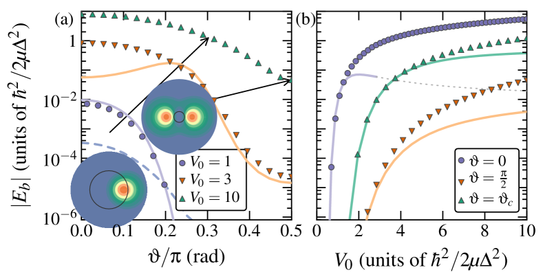
Figure 1: (Color online) Binding energy of lowest interlayer bound states in the bilayer dipolar potential Eq. (11) as a function of (a) the polarization angle from the symmetry axis and (b) interaction strength $V_{0}$. The symbols mark numerical results, the dashed line an approximation in Ref. Simon (1976) for $V_{0}=1$, and solid lines the corresponding approximation Eqs. (6)-(10). The latter approximation remains valid up to moderate $V_{0}$ as long as $|E_{b}|\ll 1$. The insets show densities of the bound states at the indicated polarization angles and $V_{0}=10$. The dark circles indicate the radius of one layer distance $\Delta$.

In Fig. 1 we plot the binding energy of the lowest lying interlayer bound states in the potential (11) as a function of the polarization angle and interaction strength. Their binding is strongest for perpendicular polarization and weakest for parallel polarization. We observe that the weak potential approximation for the binding energy, Eqs. (6)-(10), remains valid up to moderate potential strengths $V_{0}\lesssim 3$ as long as the binding energy is sufficiently small, $|E_{b}|\ll 1$. In contrast, the approximation in Ref. Simon (1976), $|E_{b}|\sim\exp(1/c)$ with $c=(1/8\pi^{2})\int d^{2}\boldsymbol{\mathrm{r}}d^{2}\boldsymbol{\mathrm{r}}^{\prime}V(\boldsymbol{\mathrm{r}})\ln|\boldsymbol{\mathrm{r}}-\boldsymbol{\mathrm{r}}^{\prime}|V(\boldsymbol{\mathrm{r}}^{\prime})$, describes the angle dependence of the binding energy only poorly. Our numerical computations are based on Netlib’s zvode solver, and we provide an explicit Jacobian for improved stability. We include partial waves up to sixth order.

As an example, we consider bosonic ⁶Li⁴⁰K molecules separated by $\Delta=200\,\mathrm{nm}$. Then the energy scale in Fig. 1 is $\hbar^{2}/2\mu\Delta^{2}\simeq 1.2\,\umu\mathrm{K}$ (units of $k_{B}$) and $V_{0}\simeq 9.5$ (cf. $V_{0}=10$ in Fig. 1), with $k_{B}$ the Boltzmann constant. Therefore, the interlayer bound state of LiK molecules should persist over a wide range of polarization angles under typical experimental temperatures in the nano-Kelvin regime. For fermionic ⁴⁰K⁸⁷Rb molecules we have $V_{0}\simeq 1$ with energy scale $\simeq 220\,\mathrm{nK}$ (units of $k_{B}$). Therefore, it can be seen from Fig. 1(a) that they require much lower temperatures. In contrast, for dipolar atoms with a magnetic dipole moment, $V_{0}\ll 1$ (e.g., ⁵²Cr). Interlayer dipoles with $V_{0}\ll 1$ bind too weakly for all polarization angles to be stable at reasonable external parameters.

The peak of the bound state wave function shifts along the $x$ axis as the polarization direction changes from perpendicular to parallel [cf. insets in Fig. 1(a)]. This is because the attractive dipole term in the DDI dominates over the quadrupole term. However, for $\vartheta>0.47\pi$, the quadrupole term dominates and two peaks develop. For parallel polarization, the dipole term vanishes and the two peaks become symmetric. In Fig. 1(a) the distance between these peaks is $\simeq 5\Delta$, typically on the order of $\umu\mathrm{m}$. If the stability requirements are fulfilled, this could simplify the creation of interlayer bound states at parallel polarization because of their greater overlap than states at perpendicular polarization. The parallel polarization bound state can be distinguished from the mainly perpendicular one in a time of flight measurement. The time-of-flight image reflects the double peak in an asymmetric momentum distribution.

III Scattering

Next we focus on the 2D scattering problem, for which $k$ is real. Then the functions $f_{mn}^{\pm}(k,r)$ attain the finite limit $f_{mn}^{\pm}(k)=\lim_{r\rightarrow\infty}f_{mn}^{\pm}(k,r)$ because the right-hand side of Eq. (3) vanishes at $r\rightarrow\infty$. In order to capture the mixing of different partial waves, it is necessary to calculate the full S-matrix. We express the partial wave components of the scattering solution as a linear combination $\psi_{mn}(k,r)=\sum_{m^{\prime}}\phi_{mm^{\prime}}(k,r)c_{m^{\prime}n}(k)$ of the regular solutions, Eq. (2). Asymptotically, we replace $f_{mm^{\prime}}^{\pm}(k,r)$ in $\phi_{mm^{\prime}}(k,r)$ with the Jost functions $f_{mm^{\prime}}^{\pm}(k)$. On the other hand, the general asymptotic scattering wave function in 2D is $\Psi(\boldsymbol{\mathrm{k}},\boldsymbol{\mathrm{r}})\rightarrow[\mathrm{e}^{\mathrm{i}\boldsymbol{\mathrm{k}}\cdot\boldsymbol{\mathrm{r}}}+a(\boldsymbol{\mathrm{k}},\boldsymbol{\mathrm{r}})\frac{\mathrm{e}^{\mathrm{i}kr}}{\sqrt{r}}]/2\pi$, where $a(\boldsymbol{\mathrm{k}},\boldsymbol{\mathrm{r}})$ is the scattering amplitude. We match the two asymptotic expressions for the scattering wave functions by expanding the first exponential in $\Psi(\boldsymbol{\mathrm{k}},\boldsymbol{\mathrm{r}})$ in terms of scaled Hankel functions. This way, we extract the S-matrix

$$S(k)=F^{+}(k)[F^{-}(k)]^{-1}$$ (12)

and the coefficients $c_{mn}(k)=[F^{-}(k)]^{-1}_{mn}$. If the potential $V(\boldsymbol{\mathrm{r}})$ is central, $S(k)$ is diagonal, with elements $\mathrm{e}^{2\mathrm{i}\delta_{m}(k)}$ and $\delta_{m}(k)$ the $m$-th partial wave phase shift.

Let us now derive approximate expressions for the phase shifts of anisotropic 2D scattering at low energies. First we introduce an iterative solution for the coefficients $f_{mn}^{\pm}(k,r)=\sum_{j=0}^{\infty}f_{mn}^{\pm(j)}(k,r)$ as a power series in the potential strength $V_{0}$. From Eq. (4) and the expression for $\phi_{mn}(k,r)$ we obtain $f_{mn}^{\pm(j+1)}(k,r)=\pm\tfrac{1}{\mathrm{i}k}\int_{0}^{r}dr^{\prime}h_{m}^{\mp}(kr^{\prime})\sum_{m^{\prime}}V_{mm^{\prime}}(r^{\prime})\phi_{m^{\prime}n}^{(j)}(k,r^{\prime})$ and $f_{mn}^{\pm(0)}(k,r)=\delta_{mn}$, with $\phi_{mn}^{(j+1)}(k,r)=-\int_{0}^{r}dr^{\prime}g_{m}(k,r,r^{\prime})\sum_{m^{\prime}}V_{mm^{\prime}}(r^{\prime})\phi_{m^{\prime}n}^{(j)}(k,r^{\prime})$ and $\phi_{mn}^{(0)}(k,r)=j_{n}(kr)\delta_{mn}$. In the remainder of this section, we consider low scattering energies such that only up to two partial waves $\ell$ and $\ell^{\prime}$ dominate the properties of the S-matrix. The phase shifts are given by $\tan 2\delta_{\ell}(k)=\mathrm{Im}S_{\ell\ell}/\mathrm{Re}S_{\ell\ell}$, where $S_{\ell\ell}$ is a diagonal matrix element of $S$ and $\delta_{\ell^{\prime}}$ is obtained by replacing $\ell\rightarrow\ell^{\prime}$. By inserting Eq. (12) we obtain the phase shifts from the Jost matrix $F^{-}$ since $F^{+}=\overline{F^{-}}$ for real $k$. Then

$$\tan 2\delta_{\ell}(k)\simeq 2\frac{\mathrm{Im}s_{\ell\ell}}{\mathrm{Re}s_{\ell\ell}}$$ (13)

with $s_{\ell\ell}=S_{\ell\ell}|\det(F^{-})|^{2}$. Using terms $f_{mn}^{-(j)}$ up to second order and expanding $s_{\ell\ell}$ to second order in $V_{0}$ we find $\mathrm{Im}(s_{\ell\ell})=-I^{(1)}_{j_{\ell}j_{\ell}}+I^{(1)}_{j_{\ell}j_{\ell}}I^{(1)}_{y_{\ell}j_{\ell}}-I^{(1)}_{j_{\ell}j_{\ell^{\prime}}}I^{(1)}_{y_{\ell^{\prime}}j_{\ell}}+2I^{(1)}_{j_{\ell}j_{\ell}}I^{(1)}_{y_{\ell^{\prime}}j_{\ell^{\prime}}}+I^{(2)}_{j_{\ell}},$ $\mathrm{Re}(s_{\ell\ell})=1+\sum_{m=\ell,\ell^{\prime}}[-2I^{(1)}_{y_{m}j_{m}}+2I^{(2)}_{y_{m}}+I^{(1)^{2}}_{j_{m}j_{m}}+I^{(1)^{2}}_{y_{m}j_{m}}]-2I^{(1)^{2}}_{j_{\ell}j_{\ell}}-2I^{(1)}_{y_{\ell}j_{\ell^{\prime}}}I^{(1)}_{y_{\ell^{\prime}}j_{\ell}}+4I^{(1)}_{y_{\ell}j_{\ell}}I^{(1)}_{y_{\ell^{\prime}}y_{\ell^{\prime}}}$, $I_{p_{m}q_{n}}^{(1)}(k)=(1/k)\int_{0}^{\infty}drp_{m}(kr)V_{mn}(r)q_{n}(kr)$, $I^{(2)}_{p_{n}}(k)=(1/k)\int_{0}^{\infty}drp_{n}(kr)\sum_{m}V_{nm}(r)\int_{0}^{r}dr^{\prime}g_{m}(k,r,r^{\prime})V_{mn}(r^{\prime})j_{n}(kr^{\prime})$ and $p_{m}$, $q_{n}$ stand in for scaled Bessel functions of order $m$ and $n$, respectively. The anisotropy of the potential enters the phase shift through mixing terms, such as $I^{(1)}_{j_{\ell}j_{\ell^{\prime}}}$, and the sum in $I^{(2)}_{p_{n}}$. These terms are absent for a central potential so we recover a result in Ref. Klawunn et al. (2010). Furthermore, for small $V_{0}$ we expand Eq. (13) to second order in $V_{0}$:

$$\tan 2\delta_{\ell}(k)\simeq-2I_{j_{\ell}j_{\ell}}^{(1)}(k)+2[I^{(2)}_{\ell}-I^{(1)}_{j_{\ell}j_{\ell}}I^{(1)}_{y_{\ell}j_{\ell}}-I^{(1)}_{j_{\ell}j_{\ell^{\prime}}}I^{(1)}_{y_{\ell^{\prime}}j_{\ell}}].$$ (14)

Thus, we recover a second-order Born approximation of the phase shift from our general formalism. We find a further approximation by considering the sum of all partial waves at small energies. For any S-matrix, $\cot\sum_{\ell}\delta_{\ell}(k)=\mathrm{Re}(\det S)/\mathrm{Im}(\det S)=-\mathrm{Re}(\det F^{-})/\mathrm{Im}(\det F^{-})$. As in the preceding section, we expand $\det F^{-}$ around $k=0$ and use the fact that $k$ is real to obtain

$$\cot\sum_{\ell}\delta_{\ell}(k)\simeq\frac{1}{\pi}\ln\left(\frac{k^{2}}{|E_{b}|}\right).$$ (15)

Here, $E_{b}$ is the binding energy, Eq. (6).

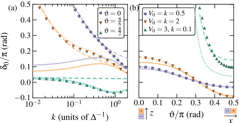
Figure 2: (Color online) S-wave phase shift for anisotropic interlayer scattering of dipoles as a function of (a) the collision momentum for $V_{0}=1$ (e.g., KRb molecules at $\Delta=200\,\mathrm{nm}$) and (b) the polarization angle. The symbols mark numerical results, solid lines the second-order Born approximation Eq. (14), dashed lines Eq. (15), and dotted lines Eq. (13) to second order in $f_{mn}^{-(j)}$. The weak potential approximation (13) describes scattering well from moderately small collision momenta and up to moderate potential strengths at all polarizations. The bound-state approximation (15) is only accurate at very low momenta and predominantly perpendicular polarization.

In Fig. 2(a) we plot the s-wave phase shift of two dipoles with $V_{0}=1$ interacting across two layers as a function of the collision momentum $k$, e.g., ⁴⁰K⁸⁷Rb with different spins at $\Delta=200\,\mathrm{nm}$. The sharp increase of the s-wave phase shift at $k\rightarrow 0$ ($\vartheta=0,\pi/6$) is a consequence of the very weakly bound states. If $\delta_{0}$ dominates in Eq. (15), a very small binding energy leads to a phase jump in $\delta_{0}$ close to $k=0$. Since the binding energy decreases strongly with increasing polarization angle, expression (15) describes the scattering of mainly in-plane polarization only at unrealistically small collision energies. On the other hand, the weak potential approximation (13) describes the numerics excellently at all considered momenta. It fails at large potential strengths $V_{0}\gg 1$ and small momenta. For large momenta $k\gg 1$ this approximation becomes identical with the Born approximation (14). In Fig. 2(b) we observe that the s-wave phase shift can vary strongly with the polarization angle at small momenta. The phase jump is caused by a weakly bound state at $\vartheta\simeq 0.3\pi$ [see Fig. 1(a)]. This variability should be observable in the scattering of polar molecules. The bound-state approximation (15) describes this behavior qualitatively even for such moderately large potential strengths as long as $k\ll 1$. The difference is mainly due to neglecting higher order partial waves in Eq. (15). For a small potential strength $V_{0}\ll 1$ our approximation Eq. (13) describes scattering excellently at all polarizations. We find that this approximation remains valid even at moderately large potential strengths $V_{0}\lesssim 3$ at higher energies $k^{2}\gtrsim 1$.

IV Conclusions

We have proposed a framework for calculating scattering and bound state properties for anisotropic 2D potentials. Our method generalizes the Jost formalism known from 3D scattering. We have derived systematic approximations for the scattering phase shifts and binding energy at low to moderate potential strengths. For weak potentials we have recovered a second-order Born approximation. The central equation (3) is also well-suited for numerical computations.

We have applied our method to polar molecules trapped in a bilayer and polarized along an arbitrary direction. We find that absolute energies of ⁶Li⁴⁰K interlayer bound states are larger than their thermal energy in ultracold experiments even for nonperpendicular polarization. The s-wave phase shift of molecules with moderate or large DDI exhibits a strong dependence on the polarization angle. These results are important, e.g., for the BEC-BCS crossover in fermionic polar molecules in bilayers Pikovski et al. (2010); Zinner et al. (2010). Varying the direction of the external polarizing field should influence the crossover from interlayer pair condensation to BCS pairing.

We thank Dieter Jaksch for helpful discussions. This work was supported by the Academic Research Fund of the Ministry of Education of Singapore, Grant No. R-146-000-120-112.