Numerical approach to multi-loop integrals

Abstract:

For the calculation of multi-loop Feynman integrals, a novel numerical method, the Direct Computation Method (DCM) is developed. It is a combination of a numerical integration and a series extrapolation. In principle, DCM can handle diagrams of arbitrary internal masses and external momenta, and can calculate integrals with general numerator function. As an example of the performance of DCM, a numerical computation of two-loop box diagrams is presented. Further discussion is given on the choice of control parameters in DCM. This method will be an indispensable tool for the higher order radiative correction when it is tested for a wider class of physical parameters and the separation of divergence is done automatically.

1 Introduction

The high-statistics data in high-energy physics requires the theoretical prediction with enough accuracy. The prediction can be given by perturbative calculation in quantum field theory. Then the multi-loop integral is an indispensable component for the theoretical study.

We define the multi-loop integrals by the following formula where the space-time dimension is denoted as $n=4-2\delta$ . Here we confine the discussion to scalar integrals only. Since the method presented below is basically numerical, the inclusion of a numerator will be straight-forward.

$${\cal I}=\int\prod_{j=1}^{L}\frac{d^{n}\ell_{j}}{(2\pi)^{n}i}\ \prod_{r=1}^{N}\frac{1}{D_{r}}$$ (1)

where the propagator is $D_{r}=q_{r}^{2}-m_{r}^{2}+i\epsilon$, $N$ is the number of propagators and $L$ is the number of loops. We combine the propagators by the standard Feynman parameter integral

$$\prod_{r=1}^{N}\frac{1}{D_{r}}=(N-1)!\int\prod dx_{r}\frac{\delta(1-\sum x_{r})}{(\sum x_{r}D_{r})^{N}}$$ (2)

and perform integration with respect to the loop momenta. We obtain

$${\cal I}=\frac{\Gamma(N-nL/2)}{(4\pi)^{nL/2}}\times I,\quad I=(-1)^{N}\int\prod dx_{r}\frac{\delta(1-\sum x_{r})}{U^{n/2}(V-i\epsilon)^{N-nL/2}}\,,$$ (3)

$$V=M^{2}-\frac{W}{U},\qquad M^{2}=\sum_{r}x_{r}m_{r}^{2}$$ (4)

where $U$ and $W$ are polynomials in the $x$ parameters[2].

In Section 2, we propose a unique method to calculate the integral $I$ in Eq.3. We call the method the Direct Computation Method (DCM). In the preceding works[3], DCM has successfully calculated one-loop and two-loop diagrams. As an example we show the results for the two-loop box diagrams in Section 3 and also report a study on the parameters in DCM. We discuss further aspects of DCM in Section 4.

2 Method

DCM consists of a regularized numerical integration and an extrapolation of a numerical sequence.

Figure 1: Integral paths for (a) analytical calculation and for (b) DCM. The cross ($\times$) stands for the singularity of integrand.

In order to illustrate the idea of regularized numerical integration, let us consider a simple integral:

$$J=\int_{0}^{1}\frac{dx}{m^{2}-sx(1-x)-i\epsilon}$$ (5)

As is shown in Fig.1, the integrand of Eq.5 has singular points when $s>4m^{2}$. Analytically, this can be handled by taking $\epsilon$ as an infinitesimal positive quantity, or, in other words, by the hyper-function formula $1/(z-i\epsilon)=P(1/z)+i\pi\delta(z)$. Numerical computation is unstable if the integrand is divergent at some points. A way to solve the situation is to deform the path in the complex $x$ plane to avoid the singular points. However, the deformation would be very complicated for the integrand of a multi-variable function. Another possibility is to assume that $\epsilon$ is a finite quantity as is shown in Fig.1(b). Then, the numerical integration along the $x$-axis is stable. If we can calculate the limiting value for $\epsilon\rightarrow 0$, it is the value of the integral $J$.

The loop integral $I(\epsilon)$ is defined by

$$I(\epsilon)=(-1)^{N}\int\prod dx_{r}\frac{\delta(1-\sum x_{r})(V+i\epsilon)^{N-nL/2}}{U^{n/2}(V^{2}+\epsilon^{2})^{N-nL/2}}\,,$$ (6)

and if $\epsilon$ and $\delta$ are finite, the numerical integration can be performed using a suitable numerical computation library.

We use $\epsilon$ determined by a (scaled) geometric sequence

$$\epsilon=\epsilon_{l}=\epsilon_{0}/(A_{c})^{l},\quad(l=0,1,\cdots)$$ (7)

for constants $\epsilon_{0},A_{c}\ (A_{c}>1)$. Then we expect

$$I=\lim_{l\rightarrow\infty}I(\epsilon_{l}).$$ (8)

Repeating the numerical integration, we obtain a sequence of numerical values of $I(\epsilon_{l})$ for $l=0,1,\ldots,l_{max}$. From these values and using an extrapolation method, we can estimate the value of $I$ with enough accuracy.

Next we discuss the singularity originating from $\delta\rightarrow 0$. In Eq.6, $V^{2}+\epsilon^{2}$ is positive and $U$ is positive semi-definite. Only at the boundary of the integration region $U$ becomes 0 . When $\delta\rightarrow+0$, it is either integrable like $\displaystyle{\int_{0}dxdy\frac{1}{(x+y)^{1-\delta}}}$ or non-integrable like $\displaystyle{\int_{0}dx\frac{1}{x^{1-\delta}}}$. In the latter case it develops a pole term $\sim 1/\delta$ as the ultraviolet singularity. Depending on the masses and external momenta, $V$ can be 0 inside the integration region to develop the imaginary part of $I$  , and also can be 0 at the boundary of integral region (as in the case of $U$) to develop an infrared singularity pole $\sim 1/\delta$. If Eq.6 is free from these singularities, we just put $\delta=0$. If not, the integral in Eq.6 is denoted as $I(\delta,\epsilon)$ and we first calculate $I(\delta)=\lim_{l\rightarrow\infty}I(\delta,\epsilon_{l})$ as in Eq.8 fixing $\delta$. Then, we assume the following form:

$$I(\delta)=\cdots+\frac{C_{-1}}{\delta}+C_{0}+C_{1}\delta+\cdots$$ (9)

We calculate $I(\delta)$ for a set of values of $\delta$ and estimate the coefficients $C_{j}$. For instance, in case of a single pole, $\delta I(\delta)=C_{-1}+C_{0}\delta+O(\delta^{2})$ and we extract $C_{-1}$ and $C_{0}$ .

So much for the description of DCM and one can understand the necessity of an efficient library for the numerical integration and that for the extrapolation. For the former we use DQAGE[4] which is a variant of Gaussian quadrature. Since it works adaptively, one can specify the accuracy of the numerical results, although the high accuracy costs in computation time. For the latter we use Wynn’s $\epsilon$ algorithm[5] which predicts the limiting value by the following iteration. We set the results of the numerical integration as initial values of the series $a(l,k)$:

$$a(l,-1)=0,\qquad a(l,0)=I(\epsilon_{l}),\qquad l=0,1,\cdots.$$ (10)

The element $a(l,k+1)$ is obtained by the following recurrence relation:

$$a(l,k+1)=a(l+1,k-1)+\frac{1}{a(l+1,k)-a(l,k)},\qquad l=0,1,\cdots.$$ (11)

Whilst the $a(l,k)$ values with odd $k$ are meant to store temporary numbers, the $a(l,k)$ with even $k$ give extrapolated estimates.

3 Numerical results

We calculate the integrals for the two-loop box diagrams shown in Fig.2. The parameters are $m_{1}=m_{2}=m_{5}=m_{6}=m=50\mathrm{GeV}$, $m_{3}=m_{4}=m_{7}=M=90\mathrm{GeV}$, $p_{1}^{2}=p_{2}^{2}=p_{3}^{3}=p_{4}^{2}=m^{2}$ and $t=(p_{1}+p_{3})^{2}=-(100)^{2}\mathrm{GeV^{2}}$. We take $s=(p_{1}+p_{2})^{2}$ variable and introduce a dimensionless variable $f_{s}=s/m^{2}$.

Figure 2: (a)Two-loop planar box diagram and (b) Two-loop non-planar box diagram. The mass of internal line $k$ is $m_{k}$. Each external momentum flows inward.

The explicit form of the $U$ and $W$ functions is found in [6]. Since there is no ultraviolet/infrared divergence, we put $\delta=0$ in Eq.3. The integral is 6-dimensional and we perform a transformation of the integration variables onto a 6-dimensional hypercube $[0,1]^{6}$. By this transformation one can cancel common variables between the numerator and the denominator. The results are presented in Fig.3 and in Fig.4. In [6], we verified the results by comparison with another computation which is a combination of algebraic transformations and numerical integration, and also by the consistency check between the real and imaginary parts through the dispersion relation.

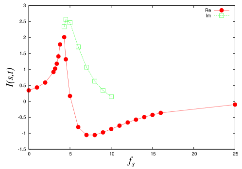
Figure 3: Numerical results of $I$ for the planar diagram in units of $10^{-12}$ ${\rm GeV}^{-6}$ for $0.0\leq f_{s}\leq 25.0$ and $t=-10000.0{\rm GeV}^{2}$. Plotted points are the real part (bullets) and the imaginary part (squares). For the latter, the region $f_{s}>10$ is not yet computed.

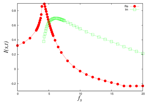
Figure 4: Numerical results of $I$ for the non-planar diagram in units of $10^{-12}$ ${\rm GeV}^{-6}$ for $0.0\leq f_{s}\leq 20.0$ and $t=-10000.0{\rm GeV}^{2}$. Plotted points are the real part (bullets) and the imaginary part (squares).

Figure 5: The real part(lower points) and imaginary part(upper points) of one-loop scalar vertex integral $I(\epsilon)$ are shown. The horizontal red line is the exact (analytical) value.

In DCM, the validity of the extrapolation depends on the choice of the values of $\epsilon$. We keep finite value of $\epsilon$ in the numerical integration, so that its physical dimension is the same as the squared mass. We have two parameters in Eq.7. $A_{c}$ is normally $A_{c}=2$ and we can use $A_{c}=1.2$ or $1.3$ to obtain a less computational intensive sequence of integrals as $\epsilon$ decreases more slowly. In order to study the choice of $\epsilon_{0}$, the initial value of the iteration, we have calculated the following on-mass-shell one-loop vertex integral as an example:

$$I=\int_{0\leq x+y\leq 1}dxdy\frac{1}{M^{2}(1-x-y)+m_{e}^{2}(x+y)^{2}-sxy-i\epsilon}$$ (12)

Here, $s=500^{2}\mathrm{GeV^{2}}$ and $m_{e}=0.5\times 10^{-3}\mathrm{GeV}$. The value of this integral is computed with a given value of $M$ and $\epsilon=1.2^{70-m}$ for $m=0,1,\ldots,120$. Then we use the values for $m,m+1,\ldots,m+14$ as the input of extrapolation. This means that we take $l_{max}=14$ and $\epsilon_{0}=1.2^{70-m}\mathrm{GeV^{2}}$ for $m=0,1,\ldots,100$.

Table.1  Extrapolated values of $I$. 15 values, $I(\epsilon_{l})=\epsilon_{0}/(1.2)^{l},\ (l=0,\ldots,14)$, are used for the extrapolation. Error is not the difference from the analytical value but estimated from the extrapolation.

$\epsilon_{0}$	Real part of $I$	error	Imaginary part of $I$	error
3.49E+05	-1.75104242540072E-05	1.65E-09	2.25556360020931E-09	1.80E-09
5.63E+04	-1.75105247961553E-05	3.02E-13	-2.96789310051170E-05	8.78E-08
9.10E+03	-1.75105248407057E-05	1.55E-14	4.35402513918612E-05	1.82E-09
1.47E+03	-1.75105250993412E-05	6.78E-21	4.34982757936633E-05	4.04E-13
2.37E+02	-1.75105250996915E-05	2.76E-16	4.34982757936633E-05	4.04E-13
3.83E+01	-1.75105250989527E-05	1.40E-17	4.34982788205288E-05	1.92E-17
6.19E+00	-1.75105250987944E-05	3.58E-18	4.34982788206820E-05	5.55E-16
1.00E+00	-1.75105251104117E-05	1.22E-15	4.34982788654878E-05	9.93E-14
1.62E-01	-1.75105250921691E-05	1.98E-16	4.34982793676347E-05	2.11E-14
2.61E-02	-1.75105251352866E-05	1.71E-15	4.34982790401757E-05	4.97E-14
4.21E-03	-1.75105251110498E-05	4.07E-15	4.34982788582295E-05	2.21E-17
(analytical)	-1.75105250974494E-05		4.34982788194091E-05

The calculated results for $M=90\mathrm{GeV}$ are shown in Fig.5 and Table.1. It is to be noted that $\epsilon$ in DCM is obviously finite. One can see that even when the value of $I(\epsilon)$ differs from the analytical value, the extrapolation gives a good estimation. There is a finite region that shows the agreement between the analytical value and the extrapolated one. This behavior demonstrates that DCM is stable up to some extent for the choice of $\epsilon_{0}$ parameters. We have tested the similar analysis for several values of $M$ ($M=1,10^{1},10^{2},10^{3}\mathrm{GeV}$) and found similar behavior. Though we need more tests for this point, we can temporally conclude that $\epsilon_{0}$ is not need to be very small but it can be set to the typical squared mass in the denominator of the integrand.

In the calculation of the two-loop box diagrams described above, we have checked the convergence of the extrapolation step-by-step. The value used for $\epsilon_{0}$ is $1.2^{40}\sim 1.2^{45}\mathrm{GeV^{2}}$ which would be consistent with the above conjecture.

4 Summary

In this paper, we have outlined DCM and calculated the two-loop scalar box integral as an example to show its applicability. Since the radiative correction in the electroweak theory (or in the SUSY model) involves various combinations of mass parameters in the integrand, DCM is a good candidate to handle general loop integrals.

In order to use DCM for the calculation of higher-order radiative corrections, we plan to proceed to the following research.

1. The method should be tested for a wider class of diagrams with various combinations of masses and external momenta and with the numerator structure.

2. Further study on the choice of parameters $\epsilon_{0},A_{c}$ is required for a stable application.

3. The variable transformation is sometimes important for good convergence. This is to be processed in an automatic manner.

4. In dimensional regularization, the ultraviolet/infrared divergence appears as a pole $1/\delta$. The separation of the infrared pole is already done successfully in [7]. A similar treatment of ultraviolet poles is expected.

5. Sometimes DCM needs long computational time. It will be important to perform the computations in a parallel computing environment.

Acknowledgements

We wish to thank Prof. T.Kaneko for his discussions and valuable comments. This work was supported in part by the Grant-in-Aid (No.20340063 and No.23540328) of JSPS and by the CPIS program of Sokendai.

References

- [1]
-
[2]
R.J.Eden, P.V.Landshoff, D.I.Olive, J.C.Polkinghorne,
The Analytic S-Matrix, Cambridge University Press, Cambridge, 1966;
G.Tiktopoulos, Phys. Rev Vol 131 (1963) 480. - [3] See [6] and references therein.
- [4] R. Piessens, E. de Doncker, C. W. Ubelhuber and D. K. Kahaner, QUADPACK, A Subroutine Package for Automatic Integration, Springer Series in Computational Mathematics. Springer-Verlag, (1983).
-
[5]
D.Shanks,
J. Math. Phys. 34 (1955) 1;
P.Wynn, Mathematical Tables Aids to Computing 10 (1956) 91; SIAM J. Numer. Anal. 3 (1966) 91. - [6] F.Yuasa, E.de Doncker, N.Hamaguchi, T.Ishikawa, K.Kato, Y.Kurihara, J.Fujimoto, Y.Shimizu, [arXiv:1112.0637/hep-ph], submitted to Comput. Phys. Commun. (2011).
- [7] E.de Doncker, J.Fujimoto, N.Hamaguchi, T.Ishikawa, Y.Kurihara, M. Ljucovic, Y.Shimizu, F.Yuasa, PoS(CPP2010)011 [arXiv:1110.3587/hep-ph], (2011).