Time-like and space-like electromagnetic form factors of nucleons, a unified description

Abstract

The extended Lomon-Gari-Krümpelmann model of nucleon electromagnetic form factors, which embodies $\rho$, $\rho^{\prime}$, $\omega$, $\omega^{\prime}$ and $\phi$ vector meson contributions and the perturbative QCD high momentum transfer behavior has been extended to the time-like region. Breit-Wigner formulae with momentum-dependent widths have been considered for broad resonances in order to have a parametrization for the electromagnetic form factors that fulfills, in the time-like region, constraints from causality, analyticity, and unitarity.

This analytic extension of the Lomon-Gari-Krümpelmann model has been used to perform a unified fit to all the nucleon electromagnetic form factor data, in the space-like and time-like region (where form factor values are extracted from $e^{+}e^{-}\leftrightarrow N\overline{N}$ cross sections data).

The knowledge of the complete analytic structure of form factors enables predictions at extended momentum transfer, and also of time-like observables such as the ratio between electric and magnetic form factors and their relative phase.

1 Introduction

Nucleon electromagnetic form factors (EMFF’s) describe modifications of the pointlike photon-nucleon vertex due to the structure of nucleons. Because the virtual photon interacts with single elementary charges, the quarks, it is a powerful probe for the internal structure of composite particles. Moreover, as the electromagnetic interaction is precisely calculable in QED, the dynamical content of each vertex can be compared with the data.
The study of EMFF’s is an essential step towards a deep understanding of the low-energy QCD dynamics. Nevertheless, even in case of nucleons, the available data are still incomplete.
The experimental situation is twofold:

• in the space-like region many data sets are available for elastic electron scattering from nucleons ($N$), both protons ($p$) and neutrons ($n$). Recently, the development of new polarization techniques (see e.g. Ref. [1]) provides an important improvement to the accuracy, giving a better capability of disentangling electric and magnetic EMFF’s than the unpolarized differential cross sections alone.

• In the time-like region there are few measurements, mainly of the total cross section (in a restricted angular range) of $e^{+}e^{-}\leftrightarrow N\overline{N}$, one set for neutrons and nine sets for protons, one of which includes a produced photon. Only two attempts, with incompatible results, have been made to separate the electric and magnetic EMFF’s in the time-like region.

Many models and interpretations for the nucleon EMFF’s have been proposed. Such a wide variety of descriptions reflects the difficulty of connecting the phenomenological properties of nucleons, parametrized by the EMFF’s, to the underlying theory which is QCD in the non-perturbative (low-energy) regime.
The analyticity requirement, which connects descriptions in both space ($q^{2}<0$) and time-like ($q^{2}>0$) regions, drastically reduces the range of models to be considered. In particular, the more successful ones in the space-like region are the Vector-Meson-Dominance (VMD) based models [2, 3] (see, e.g., Ref. [4] for a review on VMD models) that, in addition, because of their analytic form, have the property of being easily extendable to the whole $q^{2}$-domain: space-like, time-like and asymptotic regions.
In this paper we propose an analytic continuation to the time-like region of the last version of the Lomon model for the space-like nucleon EMFF’s [5]. This model has been developed by improving the original idea, due to Iachello, Jackson and Landé [2] and further developed by Gari and Krümpelmann [3], who gave a description of nucleon EMFF’s which incorporates: VMD at low momentum transfer and asymptotic freedom in the perturbative QCD (pQCD) regime. As we will see in Sec. 3, in this model EMFF’s are described by two kinds of functions: vector meson propagators, dominant at low-$q^{2}$ and hadronic form factors (FF’s) at high-$q^{2}$. The analytic extension of the model only modifies the propagator part and consists in defining more accurate expressions for propagators that account for finite-width effects and give the expected resonance singularities in the $q^{2}$-complex plane.

2 Nucleon electromagnetic form factors

The elastic scattering of an electron by a nucleon $e^{-}N\to e^{-}N$ is represented, in Born approximation, by the diagram of Fig. 1 in the vertical direction. In this kinematic region the 4-momentum of the virtual photon is space-like: $q^{2}=-2\omega_{1}\omega_{2}(1-\cos\theta_{e})\leq 0$, $\omega_{1(2)}$ is the energy of the incoming (outgoing) electron and $\theta_{e}$ is the scattering angle.

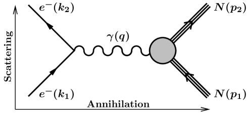
Figure 1: One-photon exchange Feynman diagram for scattering $e^{-}N\to e^{-}N$ and annihilation $e^{+}e^{-}\to N\overline{N}$.

The annihilation $e^{+}e^{-}\to N\overline{N}$ or $N\overline{N}\to e^{+}e^{-}$ is represented by the same diagram of Fig. 1 but in the horizontal direction, in this case the 4-momentum $q$ is time-like: $q^{2}=(2\omega)^{2}\geq 0$, where $\omega\equiv\omega_{1}=\omega_{2}$ is the common value of the lepton energy in the $e^{+}e^{-}$ center of mass frame.
The Feynman amplitude for the elastic scattering is

$$\mathcal{M}=\frac{1}{q^{2}}\big{[}e\,\overline{u}(k_{2})\gamma^{\mu}u(k_{1})\big{]}\big{[}e\,\overline{U}(p_{2})\Gamma_{\mu}(p_{1},p_{2})U(p_{1})\big{]}\,,$$

where the 4-momenta follow the labelling of Fig. 1, $u$ and $U$ are the electron and nucleon spinors, and $\Gamma^{\mu}$ is a non-constant matrix which describes the nucleon vertex. Using gauge and Lorentz invariance the most general form of such a matrix is [6]

$$\Gamma^{\mu}=\gamma^{\mu}F_{1}^{N}(q^{2})+\frac{i\sigma^{\mu\nu}q_{\nu}}{2M_{N}}F_{2}^{N}(q^{2})\,,$$ (1)

where $M_{N}$ is the nucleon mass ($N=n$, $p$), $F_{1}^{N}(q^{2})$ and $F_{2}^{N}(q^{2})$ are the so-called Dirac and Pauli EMFF’s, they are Lorentz scalar functions of $q^{2}$ and describe the non-helicity-flip and the helicity-flip part of the hadronic current respectively. Normalizations at $q^{2}=0$ follow from total charge and static magnetic moment conservation and are

$$F_{1}^{N}(0)=Q_{N}\,,\hskip 14.22636ptF_{2}^{N}(0)=\kappa_{N}\,,$$

where $Q_{N}$ is the electric charge (in units of $e$) and $\kappa_{N}$ the anomalous magnetic moment (in units of the Bohr magneton $\mu_{B}$) of the nucleon $N$.
In the Breit frame, i.e. when the transferred 4-momentum $q$ is purely space-like, $q=(0,\vec{q})$, the hadronic current takes the standard form of an electromagnetic 4-current, where the time and the space component are Fourier transformations of a charge and a current density respectively:

$$\left\{\begin{array}[]{l}\rho_{q}=J^{0}=\displaystyle e\left[F_{1}^{N}+\frac{q^{2}}{4M^{2}}F_{2}^{N}\right]\\ \\ \vec{J}_{q}=e\,\overline{U}(p_{2})\vec{\gamma}U(p_{1})\,[F_{1}^{N}+F_{2}^{N}]\\ \end{array}\right.\,.$$ (5)

We can define another pair of EMFF’s through the combinations

$$\left\{\begin{array}[]{l}\displaystyle G_{E}^{N}=F_{1}^{N}+\frac{q^{2}}{4M_{N}^{2}}F_{2}^{N}\\ \\ \displaystyle G_{M}^{N}=F_{1}^{N}+F_{2}^{N}\end{array}\right.$$ (9)

these are the Sachs electric and magnetic EMFF’s [7], that, in the Breit frame, correspond to the Fourier transformations of the charge and magnetic moment spatial distributions of the nucleon. The normalizations, which reflect this interpretation, are

$$G_{E}^{N}(0)=Q_{N}\,,\hskip 14.22636ptG_{M}^{N}(0)=\mu_{N}\,,$$

where $\mu_{N}=Q_{N}+\kappa_{N}$ is the nucleon magnetic moment. Moreover, Sachs EMFF’s are equal to each other at the time-like production threshold $q^{2}=4M_{N}^{2}$, i.e.:

$$G_{E}^{N}(4M_{N}^{2})=G_{M}^{N}(4M_{N}^{2})\,.$$

Finally, we can consider the isospin decomposition for the Dirac and Pauli EMFF’s

$$F^{\rm is}_{i}=\frac{1}{2}(F_{i}^{p}+F_{i}^{n})\,,\hskip 56.9055ptF^{\rm iv}_{i}=\frac{1}{2}(F_{i}^{p}-F_{i}^{n})\,,\hskip 56.9055pti=1,\,2\,,$$ (10)

$F^{\rm is}$ and $F^{\rm iv}$ are the isoscalar and isovector components.

3 The Model

The model presented here is based on simpler versions designed for the space-like EMFF’s of Iachello, Jackson and Landé [2] and of Gari and Krümpelmann idea [3], which describes nucleon EMFF’s by means of a mixture of VMD, for the electromagnetic low-energy part, and strong vertex FF’s for the asymptotic behavior of super-convergent or pQCD. The Lomon version [5], which fits well all the space-like data now available included two more well identified vector mesons and an analytic correction to the form of the $\rho$ meson propagator suitable for describing the effect of its decay width in the space-like region fitted to a dispersive analysis by Mergell, Meissner, and Drechsel [8].
This model describes the isospin components, eq. (10), in order to separate different species of vector meson contributions. For the isovector part the Lomon model used the $\rho$ and $\rho(1450)$ or $\rho^{\prime}$ contribution, while for the isoscalar the $\omega$, $\omega(1420)$ or $\omega^{\prime}$ and $\phi$ were considered. In detail these are the expressions:

$$\begin{array}[]{rcl}F^{\rm iv}_{1}(q^{2})&\!\!\!\!=\!\!\!\!&\displaystyle\big{[}BW_{\rm MMD}^{1,\rho}(q^{2})\,+BW_{0}^{\rho^{\prime}}(q^{2})\,\big{]}F_{1}^{\rho}(q^{2})+\big{[}1-BW_{\rm MMD}^{1,\rho}(0)-BW_{0}^{\rho^{\prime}}(0)\big{]}F_{1}^{D}(q^{2})\\ &\!\!\!\!\!\!\!\!&\\ F^{\rm iv}_{2}(q^{2})&\!\!\!\!=\!\!\!\!&\displaystyle\kappa_{\rho}\,\big{[}BW_{\rm MMD}^{2,\rho}(q^{2})\,+BW_{0}^{\rho^{\prime}}(q^{2})\,\big{]}F_{2}^{\rho}(q^{2})+\big{[}1-BW_{\rm MMD}^{2,\rho}(0)-BW_{0}^{\rho^{\prime}}(0)\big{]}F_{2}^{D}(q^{2})\\ &\!\!\!\!\!\!\!\!&\\ F^{\rm is}_{1}(q^{2})&\!\!\!\!=\!\!\!\!&\displaystyle\big{[}BW_{0}^{\omega}(q^{2})+BW_{0}^{\omega^{\prime}}(q^{2})\,\big{]}F_{1}^{\omega}(q^{2})+BW_{0}^{\phi}(q^{2})\,F_{1}^{\phi}(q^{2})+\\ &\!\!\!\!\!\!\!\!&\big{[}1-BW_{0}^{\omega}(0)\,-BW_{0}^{\omega^{\prime}}(0)\big{]}F_{1}^{D}(q^{2})\\ &\!\!\!\!\!\!\!\!&\\ F^{\rm is}_{2}(q^{2})&\!\!\!\!=\!\!\!\!&\displaystyle\big{[}\kappa_{\omega}\,BW_{0}^{\omega}(q^{2})\,+\kappa_{\omega^{\prime}}\,BW_{0}^{\omega^{\prime}}(q^{2})\,\big{]}F_{2}^{\omega}(q^{2})+\kappa_{\phi}\,BW_{0}^{\phi}(q^{2})\,F_{2}^{\phi}(q^{2})+\\ &\!\!\!\!\!\!\!\!&\big{[}\kappa_{\rm s}-\kappa_{\omega}\,BW_{0}^{\omega}(0)-\kappa_{\omega^{\prime}}\,BW_{0}^{\omega^{\prime}}(0)\big{]}F_{2}^{D}(q^{2})\,,\\ \end{array}$$ (20)

where:

• $BW_{0}^{\alpha}(q^{2})$ is the propagator of the intermediate vector meson $\alpha$ in pole approximation

  $$BW_{0}^{\alpha}(q^{2})=\frac{g_{\alpha}}{f_{\alpha}}\,\frac{M_{\alpha}^{2}}{M_{\alpha}^{2}-q^{2}}\,,\hskip 42.67912pt\alpha=\rho^{\prime},\omega,\omega^{\prime},\phi\,,$$ (21)

  $M_{\alpha}^{2}\,g_{\alpha}/f_{\alpha}$ are the couplings to the virtual photon and the nucleons;

• $BW_{\rm MMD}^{i,\rho}(q^{2})$ are dispersion-integral analytic approximations for the $\rho$ meson contribution in the space-like region [8]

  $$BW_{\rm MMD}^{1,\rho}(q^{2}) \!\!\!\!=\!\!\!\! \frac{1.0317+0.0875\,(1-q^{2}/0.3176)^{-2}}{2\,(1-q^{2}/0.5496)}\,,$$

  $$BW_{\rm MMD}^{2,\rho}(q^{2}) \!\!\!\!=\!\!\!\! \frac{5.7824+0.3907\,(1-q^{2}/0.1422)^{-1}}{2\,\kappa_{\rho}(1-q^{2}/0.5362)}\,;$$

• the last term in each expression of eq. (LABEL:eq:gk-ff) dominates the asymptotic QCD behavior and also normalizes the EMFF’s at $q^{2}=0$ to the charges and anomalous magnetic moments of the nucleons;

• the functions $F_{i}^{\alpha}(q^{2})$, $\alpha=\rho,\omega,\phi$ and $i=1,2$, are meson-nucleon FF’s which describe the vertices $\alpha NN$, where a virtual vector meson $\alpha$ couples with two on-shell nucleons. Noting that the same meson-nucleon FF’s are used for $\rho^{\prime}$ and $\omega^{\prime}$ as for $\rho$ and $\omega$, we have

  $$\begin{array}[]{rcl}F_{i}^{\rho,\omega}(q^{2})&=&\displaystyle f_{i}(q^{2})\equiv\frac{\Lambda_{1}^{2}}{\Lambda_{1}^{2}-q^{2}}\left(\frac{\Lambda_{2}^{2}}{\Lambda_{2}^{2}-q^{2}}\right)^{i},\hskip 28.45274pti=1,2\,,\\ &&\\ F_{1}^{\phi}(q^{2})&=&\displaystyle f_{1}(q^{2})\left(\frac{q^{2}}{q^{2}-\Lambda_{1}^{2}}\right)^{3/2}\,,\\ &&\\ F_{2}^{\phi}(q^{2})&=&\displaystyle f_{2}(q^{2})\left(\frac{\Lambda_{1}^{2}}{\mu_{\phi}^{2}}\,\frac{q^{2}-\mu_{\phi}^{2}}{q^{2}-\Lambda_{1}^{2}}\right)^{3/2}\,,\\ \end{array}$$ (27)

  where $\Lambda_{1}$ and $\Lambda_{2}$ are free parameters that represent cut-offs for the general high energy behavior and the helicity-flip respectively, and

  $$\tilde{q}^{2}=q^{2}\frac{\ln\big{[}(\Lambda_{D}^{2}-q^{2})/\Lambda_{\rm QCD}^{2}\big{]}}{\ln\big{(}\Lambda_{D}^{2}/\Lambda_{\rm QCD}^{2}\big{)}}\,,$$ (28)

  where $\Lambda_{D}$ is another free cut-off which controls the asymptotic behavior of the quark-nucleon vertex, the extra factor in $F_{i}^{\phi}(q^{2})$ imposes the Zweig rule;

• the functions $F_{i}^{D}(q^{2})$ can be interpreted as quark-nucleon FF’s that parametrize the direct coupling of the virtual photon to the valence quarks of the nucleons,

  $$F_{i}^{D}(q^{2})=\frac{\Lambda_{D}^{2}}{\Lambda_{D}^{2}-\tilde{q}^{2}}\left(\frac{\Lambda_{2}^{2}}{\Lambda_{2}^{2}-\tilde{q}^{2}}\right)^{i},\hskip 28.45274pti=1,2\,,$$ (29)

  $\tilde{q}^{2}$ is defined as in eq. (28);

• finally, $\kappa_{\alpha}$ is the ratio of tensor to vector coupling at $q^{2}=0$ in the $\alpha NN$ matrix element, while the isospin anomalous magnetic moments are

  $$\kappa_{\rm s}=\kappa_{p}+\kappa_{n}\,,\hskip 56.9055pt\kappa_{\rm v}=\kappa_{p}-\kappa_{n}\,.$$

The space-like asymptotic behavior ($q^{2}\to-\infty$) for the Dirac and Pauli EMFF’s of eq. (LABEL:eq:gk-ff) is driven by the $F_{1,2}^{D}(q^{2})$ contribution, given in eq. (29). In particular we get

$$\begin{array}[]{rcl}F_{1}^{\rm iv,is}(q^{2})&\displaystyle\mathop{\sim}_{q^{2}\to-\infty}&\displaystyle\frac{1}{\Big{[}q^{2}\ln\big{(}-q^{2}/\Lambda_{\rm QCD}^{2}\big{)}\Big{]}^{2}}\\ &&\\ F_{2}^{\rm iv,is}(q^{2})&\displaystyle\mathop{\sim}_{q^{2}\to-\infty}&\displaystyle\frac{F_{1}^{\rm iv,is}(q^{2})}{-q^{2}\ln\big{(}-q^{2}/\Lambda_{\rm QCD}^{2}\big{)}}\,,\\ \end{array}$$ (33)

as required by the pQCD [9].
In principle this model can be extended also to the time-like region, positive $q^{2}$, to describe data on cross sections for the annihilation processes: $e^{+}e^{-}\leftrightarrow N\overline{N}$. However, a simple analytic continuation of the expressions given in eq. (LABEL:eq:gk-ff) involves important issues mainly concerning the analytic structure of the vector meson components of the EMFF’s that, in the time-like region, are complex functions of $q^{2}$. The hadronic FF’s of eqs. (27) and (29) may also have real poles as a function of $q^{2}$. In fact as defined above $F_{i}^{\phi}$ has a real pole at $q^{2}=\Lambda_{i}^{2}$. In the other denominators of eqs. (27) and (29), as in $F_{i}^{\rho,\omega}$ and $F_{1}^{D}$, $q^{2}$ is replaced by $\tilde{q}^{2}$. The latter as a function of $q^{2}$ has a maximum in its real range $0<q^{2}<\Lambda_{D}^{2}$, which, for reasonable values of $\Lambda_{D}$ and $\Lambda_{\rm QCD}$, may be smaller than $\Lambda_{1}^{2}$, $\Lambda_{2}^{2}$ and $\Lambda_{D}^{2}$. Therefore all the hadronic FF’s real poles may be avoided by also replacing $q^{2}$ by $\tilde{q}^{2}$ in the factors of $F_{i}^{\phi}$. This does not effect the asymptotic behavior required by the Zweig rule and will be adopted in the model used here. The results in Sec. 6 show that with this modification real poles can be avoided in every case examined, although in half the cases mild constraints on $\Lambda_{1}$ or $\Lambda_{\rm QCD}$ are needed which affect the quality of the fit negligibly.
A detailed treatment of the possibility of extending the model from the space-like to the time-like region, will be given in Sec. 5.

4 Analyticity of Breit-Wigner formulae

The standard relativistic Breit-Wigner (BW) formula for an unstable particle of mass $M$ and energy independent width $\Gamma$ is

$$BW(s)=\frac{1}{M^{2}-s-i\,\Gamma\,M}\,,$$

it has a very simple analytic structure, only one complex pole and no discontinuity cut in its domain. Once this formula is improved to include energy dependent widths one immediately face problems concerning the analyticity.
We consider explicitly the case of the $\rho$ resonance in its dominant decay channel $\pi^{+}\pi^{-}$. A realistic way to formulate an energy dependent width is to extend the $\rho$ mass off-shell, making the substitution $M_{\rho}^{2}=s$, in the first order decay rate

$$\Gamma(\rho\to\pi^{+}\pi^{-})=\frac{|g^{\rho}_{\pi\pi}|^{2}}{48\pi}\,\frac{M_{\rho}^{2}-4M_{\pi}^{2}}{M_{\rho}^{2}}\,,$$ (34)

where $g^{\rho}_{\pi\pi}$ is the coupling constant and, $M_{\rho}$ and $M_{\pi}$ are the $\rho$ and pion mass respectively. Such a decay rate has been obtained by considering, for the vertex $\rho\pi^{+}\pi^{-}$, the pointlike amplitude

$$\mathcal{M}=g^{\rho}_{\pi\pi}\,\epsilon_{\mu}\,(p_{+}-p_{-})^{\mu}\,,$$

where $\epsilon_{\mu}$ is the polarization vector of the vector meson $\rho$, and $p_{\pm}$ the 4-momentum of $\pi^{\pm}$.
Finally, assuming the $\pi^{+}\pi^{-}$ as the only decay channel and using eq. (34) for the corresponding rate, the energy dependent width can be defined as

$$\Gamma^{\rho}_{s}(s)=\Gamma^{\rho}_{0}\,\frac{M_{\rho}^{2}}{s}\left(\frac{s-s_{0}}{M_{\rho}^{2}-s_{0}}\right)^{\frac{3}{2}}\equiv\frac{\gamma_{\rho}}{M_{\rho}}\,\frac{\left(s-s_{0}\right)^{\frac{3}{2}}}{s}\,,\hskip 28.45274pt\gamma_{\rho}\equiv\frac{\Gamma^{\rho}_{0}M_{\rho}^{3}}{(M_{\rho}^{2}-s_{0})^{\frac{3}{2}}}\,,$$ (35)

where the subscript “$s$” indicates the factor $1/s$ appearing in the width definition, $\Gamma^{\rho}_{0}$ is the total width of the $\rho$, and $s_{0}=4M_{\pi}^{2}$. It follows that the BW formula becomes

$$BW_{s}(s)=\frac{s}{s(M_{\rho}^{2}-s)-i\gamma_{\rho}\,\left(s-s_{0}\right)^{\frac{3}{2}}}\,.$$

In this form the BW has the “required” [10] discontinuity cut $(s_{0},\infty)$ and maintains a complex pole $s_{p}$

$$s_{p}=\tilde{}M_{\rho}^{2}+i\tilde{}\Gamma^{\rho}_{0}\,\tilde{}M_{\rho}\simeq M_{\rho}^{2}+i\Gamma^{\rho}_{0}\,M_{\rho}=s^{0}_{p}\,.$$

Due to the more complex analytic structure the new pole position $s_{p}$ turns out to be slightly shifted with respect to the original position $s_{p}^{0}$. Moreover, these are not the only complications introduced by using $\Gamma^{\rho}(s)$ instead of $\Gamma^{\rho}_{0}$, the power 3/2 in the denominator and the factor $1/s$, see eq. (35), generate also additional physical poles which, in agreement with dispersion relations, must be subtracted, as discussed below.

4.1 Regularization of Breit-Wigner formulae

We consider the general case where there is a number $N$ of poles lying in the physical Riemann sheet. We may rewrite the BW by separating the singular and regular behaviors as

$$BW(s)=\frac{P_{N}(s)}{\prod_{j=1}^{N}(s-z_{j})\big{[}M^{2}-s-i\gamma(s-s_{0})^{\beta}\big{]}}\,,$$

where $P_{N}(s)$ is a suitable $N$ degree polynomial, $\beta$ is a non-integer real number which defines the discontinuity cut (in the previous case we had $\beta=3/2$), $\gamma=M\,\Gamma^{0}/(M^{2}-s_{0})^{\beta}$, and the $z_{j}$ are the real axis (physical) poles. To avoid divergences in our formulae, we may define a simple regularization procedure consisting in subtracting these poles. In other words we add counterparts that at $z=z_{j}$ behave as the opposite of the $i$-th pole. In more detail, we may define a regularized BW as

$$\widetilde{BW}(s)=BW(s)-\sum_{k=1}^{N}\frac{P_{N}(z_{k})}{\prod_{j=1,j\not=k}^{N}(z_{k}-z_{j})\big{[}{M}^{2}-z_{k}-i\gamma(z_{k}-s_{0})^{\beta}\big{]}}\,\frac{1}{s-z_{k}}\,.$$ (36)

In the Appendix A we show how dispersion relations (DR’s) offer a powerful tool to implement this procedure without the need to know where the poles are located. However in this paper we show that an analytic expression also contains the information.

4.2 Two cases for $\Gamma(s)$

In our model for nucleon EMFFs, widths are used only for the broader resonances: $\rho(770)$, $\rho(1450)$ and $\omega(1420)$ [11]. We consider explicitly two expressions for $\Gamma(s)$ which entail different analytic structures for the BW formulae. Besides the form we discussed in Sec. 4, eq. (35), we consider also a simpler expression (closer to the non-relativistic form), hence for a generic broad resonance we have

$$\begin{array}[]{lrl}\displaystyle\Gamma_{s}(s)=\Gamma_{0}\,\frac{M^{2}}{s}\left(\frac{s-\tilde{s}_{0}}{M^{2}-\tilde{s}_{0}}\right)^{\frac{3}{2}}\equiv\frac{\gamma_{s}}{M}\,\frac{\left(s-\tilde{s}_{0}\right)^{\frac{3}{2}}}{s}\,,&&\mbox{with: }\displaystyle\gamma_{s}=\frac{\Gamma_{0}M^{3}}{\left(M^{2}-\tilde{s}_{0}\right)^{\frac{3}{2}}}\\ &&\\ \displaystyle\Gamma_{1}(s)=\Gamma_{0}\left(\frac{s-\tilde{s}_{0}}{M^{2}-\tilde{s}_{0}}\right)^{\frac{3}{2}}\equiv\frac{\gamma_{1}}{M}\,\left(s-\tilde{s}_{0}\right)^{\frac{3}{2}}\,,&&\mbox{with: }\displaystyle\gamma_{1}=\frac{\Gamma_{0}M}{\left(M^{2}-\tilde{s}_{0}\right)^{\frac{3}{2}}}\,.\\ \end{array}$$ (40)

In both cases we assume that such a resonance decays predominantly into a two-body channel whose mass squared equals $\tilde{s}_{0}$. The subscript “1” in the second expression of eq. (40) indicates that there is no extra factor $1/s$ in the definition of the energy-dependent width.
As already discussed, the BW formulae acquire a more complex structure as functions of $s$, as a consequence unwanted poles are introduced. Such poles spoil analyticity, hence they must be subtracted by hand or, equivalently, using the DR procedure defined in Appendix A.
More in detail, for both BW formulae we have only one real pole, that we call $s_{s}$ and $s_{1}$ respectively (both less than $\tilde{s}_{0}$). The corresponding residues, that we call $R_{s,1}$, are

$$\begin{array}[]{l}\displaystyle R_{s}=\frac{s_{s}}{M^{2}-2s_{s}+\frac{3}{2}\gamma_{s}\sqrt{\tilde{s}_{0}-s_{s}}}\,,\\ \\ \displaystyle R_{1}=\frac{1}{-1+\frac{3}{2}\gamma_{1}\sqrt{\tilde{s}_{0}-s_{1}}}\,.\\ \end{array}$$ (44)

Following eq. (36), the regularized BW formulae read

$$\widetilde{BW}_{s,1}(s)=BW_{s,1}(s)-\frac{R_{s,1}}{s-s_{s,1}}\,.$$

In particular, below the threshold $\tilde{s}_{0}$, where BW’s are real, we have

$$\begin{array}[]{l}\displaystyle\widetilde{BW}_{s}(s<\tilde{s}_{0})=\frac{s}{s(M^{2}-s)-\gamma_{s}(\tilde{s}_{0}-s)^{3/2}}-\frac{R_{s}}{s-s_{s}}\,,\\ \\ \displaystyle\widetilde{BW}_{1}(s<\tilde{s}_{0})=\frac{1}{M^{2}-s-\gamma_{1}(\tilde{s}_{0}-s)^{3/2}}-\frac{R_{1}}{s-s_{1}}\,.\\ \end{array}$$ (48)

Above $\tilde{s}_{0}$ BW’s become complex, real and imaginary parts are obtained as limit of $\widetilde{B}W_{s,1}(s)$ over the upper edge of the cut $(\tilde{s}_{0},\infty)$. Since the poles $s_{s,1}$ are real only the real parts have to be corrected as

$$\begin{array}[]{l}\displaystyle\mbox{Re}\left[\widetilde{BW}_{s}(s>\tilde{s}_{0})\right]=\frac{s^{2}(M^{2}-s)}{s^{2}(M^{2}-s)^{2}+\gamma_{s}^{2}(s-\tilde{s}_{0})^{3}}-\frac{R_{s}}{s-s_{s}}\,,\\ \\ \displaystyle\mbox{Re}\left[\widetilde{BW}_{1}(s>\tilde{s}_{0})\right]=\frac{M^{2}-s}{(M^{2}-s)^{2}+\gamma_{1}^{2}(s-\tilde{s}_{0})^{3}}-\frac{R_{1}}{s-s_{1}}\,,\\ \end{array}$$ (52)

while the imaginary parts remain unchanged

$$\begin{array}[]{l}\displaystyle\mbox{Im}\left[\widetilde{BW}_{s}(s>\tilde{s}_{0})\right]=\frac{s\gamma_{s}(s-\tilde{s}_{0})^{3/2}}{s^{2}(M^{2}-s)^{2}+\gamma_{s}^{2}(s-\tilde{s}_{0})^{3}}\,,\\ \\ \displaystyle\mbox{Im}\left[\widetilde{BW}_{1}(s>\tilde{s}_{0})\right]=\frac{\gamma_{1}(s-\tilde{s}_{0})^{3/2}}{(M^{2}-s)^{2}+\gamma_{1}^{2}(s-\tilde{s}_{0})^{3}}\,.\\ \end{array}$$ (56)

Resonance	$M$ (GeV)	$\Gamma_{0}$ (GeV)	$\tilde{s}_{0}$	$s_{s}$ (GeV2)	$s_{1}$ (GeV2)
$\rho(770)$	0.7755	0.1491	$4M_{\pi}^{2}$	0.005953	-11.63
$\rho(1450)$	1.465	0.400	$4M_{\pi}^{2}$	0.003969	-29.43
$\omega(1420)$	1.425	0.215	$(M_{\pi}+M_{\rho})^{2}$	0.06239	-19.46

Table 1: Parameters for the BW formulae of resonances: $\rho(770)$, $\rho(1450)$ and $\omega(1420)$.

The parameters of the subtracted poles for the three vector mesons are reported in Table 1. A third case is discussed in Appendix B. It is not fitted to the data because its resonance structure is intermediate between the two above cases.

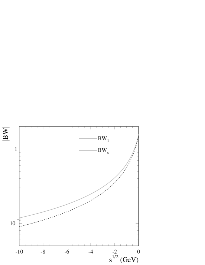
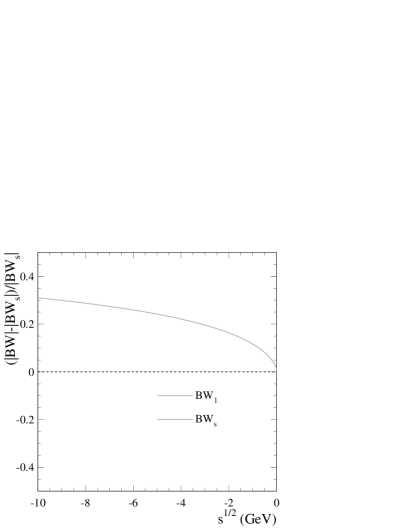
Figure 2: Left: comparison between the two descriptions of the $\rho$ peak in the space-like region. Right: relative differences w.r.t. $BW_{s}$.

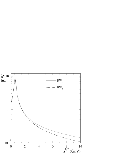
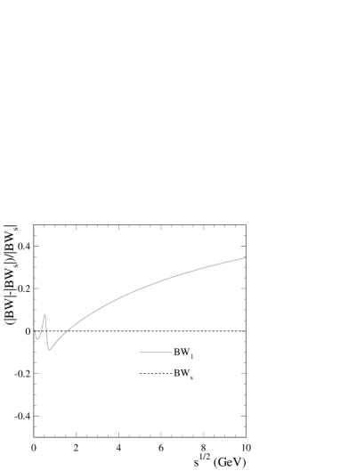
Figure 3: Left: comparison between the two descriptions of the $\rho$ peak in the time-like region. Right: relative differences w.r.t. $BW_{s}$.

Figures 2 and 3 show comparisons between the two descriptions in case of $\rho$ in the space-like and time-like regions respectively. On the left of each figure is the modulus of each, on the right the relative difference with respect to $BW_{s}$.

5 The analytic extension

The original model, described in Sec. 3 and constructed in the space-like region, can be analytically continued in the time-like region using the regularized BW formulae obtained in Sec. 4. We consider then a new set of expressions for $F^{\rm iv}_{1,2}(q^{2})$ and $F^{\rm is}_{1,2}(q^{2})$, homologous to those of eq. (LABEL:eq:gk-ff) where now we use regularized BW formulae instead of the MMD [8] $\rho$ width form or the zero-width approximation given in eq. (21), and also two additional vector meson contributions, $\rho(1450)$ and $\omega(1420)$ here simply $\rho^{\prime}$ and $\omega^{\prime}$, as in the last version of the Lomon model [5]. Such BW’s have the expected analytic structure and reproduce in both space-like and time-like regions the finite-width effect of broad resonances. The narrow widths of the $\omega$ and $\phi$ have negligible effects, so we use these modified propagators only for broader vector mesons, namely: the isovectors $\rho$ and $\rho^{\prime}$, and the isoscalar $\omega^{\prime}$. These are the new expressions for the isospin components of nucleon EMFF’s

$$\begin{array}[]{rcl}F^{\rm iv}_{1,\rm case}(q^{2})&=&\displaystyle\big{[}\widetilde{BW}_{\rm case}^{\rho}(q^{2})+\widetilde{BW}_{\rm case}^{\rho^{\prime}}(q^{2})\big{]}F_{1}^{\rho}(q^{2})\vspace{2mm}\\ &&\displaystyle+\big{[}1-\widetilde{BW}_{\rm case}^{\rho}(0)-\widetilde{BW}_{\rm case}^{\rho^{\prime}}(0)\big{]}F_{1}^{D}(q^{2})\\ &&\\ F^{\rm iv}_{2,\rm case}(q^{2})&=&\displaystyle\big{[}\kappa_{\rho}\,\widetilde{BW}_{\rm case}^{\rho}(q^{2})+\kappa_{\rho^{\prime}}\,\widetilde{BW}_{\rm case}^{\rho^{\prime}}(q^{2})\big{]}F_{2}^{\rho}(q^{2})\vspace{2mm}\\ &&\displaystyle+\big{[}\kappa_{\rm v}-\kappa_{\rho}\,\widetilde{BW}_{\rm case}^{\rho}(0)-\kappa_{\rho^{\prime}}\,\widetilde{BW}_{\rm case}^{\rho^{\prime}}(0)\big{]}F_{2}^{D}(q^{2})\\ &&\\ F^{\rm is}_{1,\rm case}(q^{2})&=&\displaystyle\big{[}BW_{0}^{\omega}(q^{2})+\widetilde{BW}_{\rm case}^{\omega^{\prime}}(q^{2})\big{]}F_{1}^{\omega}(q^{2})+BW_{0}^{\phi}(q^{2})\,F_{1}^{\phi}(q^{2})+\vspace{2mm}\\ &&\big{[}1-BW_{0}^{\omega}(0)-\widetilde{BW}_{\rm case}^{\omega^{\prime}}(0)\big{]}F_{1}^{D}(q^{2})\\ &&\\ F^{\rm is}_{2,\rm case}(q^{2})&=&\displaystyle\big{[}\kappa_{\omega}\,BW_{0}^{\omega}(q^{2})+\kappa_{\omega^{\prime}}\,\widetilde{BW}_{\rm case}^{\omega^{\prime}}(q^{2})\big{]}F_{2}^{\omega}(q^{2})+\kappa_{\phi}\,BW_{0}^{\phi}(q^{2})\,F_{2}^{\phi}(q^{2})+\vspace{2mm}\\ &&\big{[}\kappa_{\rm s}-\kappa_{\omega}\,BW_{0}^{\omega}(0)-\kappa_{\omega^{\prime}}\,\widetilde{BW}_{\rm case}^{\omega^{\prime}}(0)-\kappa_{\phi}\,BW_{0}^{\phi}(0)\big{]}F_{2}^{D}(q^{2})\,,\\ \end{array}$$

where case=$s$ and case=1 correspond to the parametrizations of the energy dependent width described in Sec. 4.2. Following eqs. (48)-(56) for the definition of $\widetilde{BW}(q^{2})$, and including the coupling constants, we have

$$\widetilde{BW}^{\beta}_{\rm case}(q^{2})=\left\{\begin{array}[]{lcl}\displaystyle\frac{g_{\beta}M^{2}_{\beta}}{f_{\beta}}\left[\frac{q^{2}}{q^{2}(M^{2}_{\beta}-q^{2})-i\gamma_{s}^{\beta}(q^{2}-\tilde{s}_{0}^{\beta})^{3/2}}-\frac{R_{s}^{\beta}}{q^{2}-s_{s}^{\beta}}\right]&&{\rm case}=s\\ &&\\ \displaystyle\frac{g_{\beta}M^{2}_{\beta}}{f_{\beta}}\left[\frac{1}{M^{2}_{\beta}-q^{2}-i\gamma_{1}^{\beta}(q^{2}-\tilde{s}_{0}^{\beta})^{3/2}}-\frac{R_{1}^{\beta}}{q^{2}-s_{1}^{\beta}}\right]&&{\rm case}=1\\ \end{array}\right.$$ (72)

with: $\beta=\rho$, $\rho^{\prime}$, $\omega^{\prime}$ (parameters in Table 1) and where: the $\gamma_{1,s}^{\beta}$ are given in eq. (40) and the residues $R_{1,s}^{\beta}$ in eq. (44). The introduction of the regularized BW’s does not spoil the high-energy behavior of the resulting nucleon EMFF’s. In fact, as $|q^{2}|\to\infty$, the function $\widetilde{BW}^{\beta}_{\rm case}(q^{2})$ vanishes like $1/q^{2}$, i.e. following the same power law as the previous $BW^{\beta}_{0}(q^{2})$, in the case=1 and case=$s$, see eq. (21), indeed we have

$$\widetilde{BW}^{\beta}_{\rm case}(q^{2})\mathop{\sim}_{|q^{2}|\to\infty}\left\{\begin{array}[]{lcl}\displaystyle\frac{g_{\beta}M^{2}_{\beta}}{f_{\beta}}\,\frac{1-R_{s}^{\beta}}{q^{2}}&&{\rm case}=s\\ &&\\ \displaystyle-\frac{g_{\beta}M^{2}_{\beta}}{f_{\beta}}\,\frac{R_{1}^{\beta}}{q^{2}}&&{\rm case}=1\\ \end{array}\right.\,.$$ (76)

It is interesting to notice that in both cases is just the subtracted pole which ensures the expected behavior and, in particular, the asymptotic limit of: $q^{2}\cdot\widetilde{BW}^{\beta}_{\rm case}(q^{2})$ is proportional to $R^{\beta}_{1}$ and $(1-R^{\beta}_{s})$ respectively. For the reason discussed at the end of Sec. 3, for the present model $q$ is replaced by $\tilde{q}$ in the hadronic FF’s $F_{i}^{\phi}$ of eq. (27).

6 Results

Nine sets of data have been considered, six of them lie in the space-like region [12] and three in the time-like region [13, 14, 15, 16, 17, 18, 19, 20, 21]. The data determine the Sachs EMFF’s and their ratios. The fit procedure consists in defining a global $\chi^{2}$ as a sum of nine contributions, one for each set. More in detail, we minimize the quantity

$$\chi^{2}=\sum_{i=1}^{9}\tau_{i}\cdot\chi^{2}_{i}\,,$$

where the coefficients $\tau_{i}$ weight the $i^{\rm th}$ contribution, we use $\tau_{i}=1$ or $\tau_{i}=0$ to include or exclude the $i^{\rm th}$ data set. The single contribution, $\chi^{2}_{i}$, is defined in the usual form as

$$\chi^{2}_{i}=\sum_{k=1}^{N_{i}}\left(\frac{Q_{i}(q^{2}_{k})-v^{i}_{k}}{\delta v^{i}_{k}}\right)^{2}\,,$$

where $Q_{i}(q^{2})$ indicates the physical observable, function of $q^{2}$, that has been measured and the set $\{q^{2}_{k},v^{i}_{k},\delta v^{i}_{k};N_{i}\}$ represents the corresponding data; $v^{i}_{k}$ is the $k^{\rm th}$ value ($k=1,\ldots,N_{i}$) of the quantity $Q_{i}$ ($i=1,\ldots,9$) measured at $q^{2}=q^{2}_{k}$, with error $\delta v^{i}_{k}$.

	$Q_{i}$	$N_{i}$	minimum $\chi^{2}_{i}$
			case = $s$ With BABAR	case = 1 With BABAR	case = $s$ No BABAR	case = 1 No BABAR
space-like	$G_{M}^{p}$	68	48.7	50.1	54.6	60.8
	$G_{E}^{p}$	36	30.4	27.6	26.2	35.0
	$G_{M}^{n}$	65	154.6	154.2	158.2	167.0
	$G_{E}^{n}$	14	22.7	23.2	24.1	26.0
	$\mu_{p}G_{E}^{p}/G_{M}^{p}$	25	13.9	12.9	10.6	14.4
	$\mu_{n}G_{E}^{n}/G_{M}^{n}$	13	11.3	10.7	8.2	8.9
​​time-like	$|G_{\rm eff}^{p}|$	81 (43)	162.5	166.7	62.2	35.0
	$|G_{\rm eff}^{n}|$	5	8.4	6.3	3.2	0.3
	Total	313(275)	452.5	451.7	347.3	347.4

Table 2: Measured quantities, numbers of data points and $\chi^{2}$ contributions. The values in parentheses indicate the number of data points in the case “No BABAR”.

Table 2 reports the complete list of observables, the number of data points and the corresponding minimum $\chi^{2}$’s, in the two considered cases as described in Sec. 5 for the sets of data with and without the BABAR data which have a final state photon. For case=$s$, with and without the BABAR data, the optimization over the full set of 13 free parameters (Table 3) determines $\Lambda_{1}$, $\Lambda_{2}$, $\Lambda_{D}$ and $\Lambda_{\rm QCD}$ such that the hadronic FF’s have no real poles. For the case=$1$ with BABAR data the full minimization implies a zero for $(\Lambda_{1}^{2}-\tilde{q}^{2})$ producing poles in the hadronic FF. Re-minimizing with the constraint $\Lambda_{1}=0.5\,{\rm GeV}$, just above the $0.4744\,{\rm GeV}$ obtained without the constraint, removes the poles. For case=$1$ without BABAR data it is required that the already fixed $\Lambda_{\rm QCD}=0.15\,{\rm GeV}$ be changed to $\Lambda_{\rm QCD}=0.10\,{\rm GeV}$ to avoid a zero of $(\Lambda_{1}^{2}-\tilde{q}^{2})$. In both cases the change in $\chi^{2}$ is negligible.
Data and fits, black and gray curves correspond to case=1 and case=$s$ respectively, are shown in Figs. 5-13. In the space-like region the electric Sachs EMFF’s are normalized to the dipole form

$$G_{D}(q^{2})=\left(1-\frac{q^{2}}{0.71\,{\rm GeV}^{2}}\right)^{-2}\,,$$

while magnetic EMFF’s are also normalized to the magnetic moment. This normalization decreases the range of variation, but the curves clearly demonstrate deviations from the dipole form. The observable $R_{N}$ is defined as the ratio $R_{N}=G_{E}^{N}/G_{M}^{N}$ for the nucleon $N$. As $N$ stands for both neutron and proton there are six space-like observables. A departure from scaling is shown in the deviation of $R_{p}$ and $R_{n}$ from unity.
The time-like effective FF, $|G_{\rm eff}^{N}|$, is defined as

$$|G_{\rm eff}^{N}(q^{2})|=\left[\frac{\sigma(e^{+}e^{-}\to N\overline{N})}{\frac{4\pi\alpha^{2}}{3q^{2}}\sqrt{1-\frac{4M_{N}^{2}}{q^{2}}}\left(1+\frac{2M_{N}^{2}}{q^{2}}\right)}\right]^{1/2}\,,$$ (77)

where $\sigma(e^{+}e^{-}\to N\overline{N})$ is the measured total cross section and the kinematic factor at denominator is the Born cross section for a pointlike nucleon. In terms of electric and magnetic EMFF’s, $G_{E}^{N}$ and $G_{M}^{N}$, i.e. considering the matrix element given in eq. (1) and the definitions of eq. (9), we have

$$|G_{\rm eff}^{N}(q^{2})|=\left(\big{|}G_{M}^{N}(q^{2})\big{|}^{2}+\frac{2M_{N}^{2}}{q^{2}}\big{|}G_{E}^{N}(q^{2})\big{|}^{2}\right)^{1/2}\left(1+\frac{2M_{N}^{2}}{q^{2}}\right)^{-1/2}\,,$$

and this is the relation that we use to fit the data on $|G_{\rm eff}^{N}|$ for both proton-antiproton and neutron-antineutron production.
The proton-antiproton production experiments were of two types, 1) the exclusive pair production [13, 14, 15, 16, 17, 18, 19, 20] and 2) production of the pair with a photon [21]. In the latter case the pair production energy is obtained by assuming that the photon was produced by the electron or positron and that no other photons were emitted but undetected. Fits of the model were made both with and without the latter data [21]. In Figs. 5-13 the fit curves corresponding to the two possibilities: with and without BABAR data, are shown as solid and dashed lines, respectively.
The free parameters of this model are:

• the three cut-offs: $\Lambda_{1}$, $\Lambda_{2}$ and $\Lambda_{D}$ which parameterize the effect of hadronic FF’s and control the transition from non-perturbative to perturbative QCD regime in the $\gamma NN$ vertex;

• five pairs of vector meson anomalous magnetic moments and photon couplings $(\kappa_{\alpha},g_{\alpha}/f_{\alpha})$, with $\alpha=\rho$, $\rho^{\prime}$, $\omega$, $\omega^{\prime}$, $\phi$.

The best values for these 13 free parameters together with the constants of this model are reported in Table 3.
The fixed parameters concern well known measurable features of the intermediate vector mesons and dynamical quantities. Particular attention has to be paid to $\Lambda_{\rm QCD}$. In fact we use the values $\Lambda_{\rm QCD}=0.15$ GeV in all cases but for the case=1 without BABAR data, where instead: $\Lambda_{\rm QCD}=0.10$ GeV. The use of such a reduced value is motivated by the requirement of having no real poles in meson-nucleon and quark-nucleon FF’s (Sec. 3). As $\Lambda_{\rm QCD}=0.15\,{\rm GeV}$ is closer to the values preferred by high energy experiments, it suggests that case=$s$ is the more physical model. Another reason to prefer it on physical grounds is that the width formula of the vector meson decay in case=s is determined by relativistic perturbation theory. Case=1 was chosen because it is a simpler relativistic modification of the non-relativistic Breit-Wigner form. This in our view is a less physical reason.

Parameter	case = $s$ With BABAR	case = 1 With BABAR	case = $s$ No BABAR	case = 1 No BABAR
$g_{\rho}/f_{\rho}$	2.766	2.410	0.9029	0.4181
$\kappa_{\rho}$	-1.194	-1.084	0.8267	0.6885
$M_{\rho}$ (GeV)	0.7755 (fixed)
$\Gamma_{\rho}$ (GeV)	0.1491 (fixed)
$g_{\omega}/f_{\omega}$	-1.057	-1.043	-0.2308	-0.4894
$\kappa_{\omega}$	-3.240	-3.317	-9.859	-1.398
$M_{\omega}$ (GeV)	0.78263 (fixed)
$g_{\phi}/f_{\phi}$	0.1871	0.1445	­0.0131	­0.1156
$\kappa_{\phi}$	-2.004	-­3.045	37.218	-0.2613
$M_{\phi}$ (GeV)	1.019 (fixed)
$\mu_{\phi}$ (GeV)	20.0 (fixed)
$g_{\omega^{\prime}}/f_{\omega^{\prime}}$	2.015	1.974	1.265	1.649
$\kappa_{\omega^{\prime}}$	­-2.053	­-2.010	­-2.044	­-0.6712
$M_{\omega^{\prime}}$ (GeV)	1.425 (fixed)
$\Gamma_{\omega^{\prime}}(GeV)$	0.215 (fixed)
$g_{\rho^{\prime}}/f_{\rho^{\prime}}$	­-3.475	­-3.274	­-0.8730	­-0.0369
$\kappa_{\rho^{\prime}}$	­-1.657	-­1.724	­-2.832	­-104.35
$M_{\rho^{\prime}}$ (GeV)	1.465 (fixed)
$\Gamma_{\rho^{\prime}}$ (GeV)	0.400 (fixed)
$\Lambda_{1}$ (GeV)	0.4801	0.5000	0.6474	0.6446
$\Lambda_{2}$ (GeV)	3.0536	3.0562	3.0872	3.6719
$\Lambda_{D}$ (GeV)	0.7263	0.7416	0.8573	0.8967
$\Lambda_{\rm QCD}$ (GeV)	0.150			0.100

Table 3: Best values of fit parameters and constants.

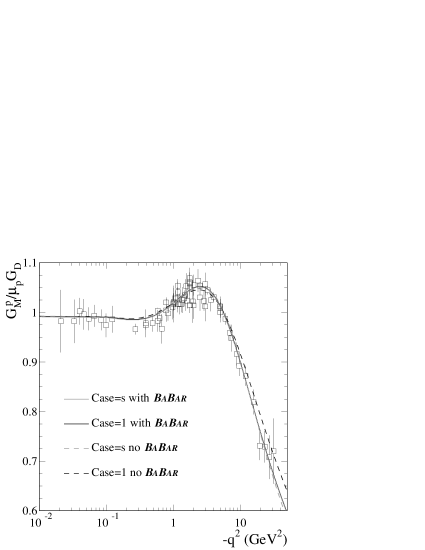
Figure 4: Space-like magnetic proton EMFF normalized to the dipole and $\mu_{p}$, in case=1 and case=$s$, including and not the BABAR data.

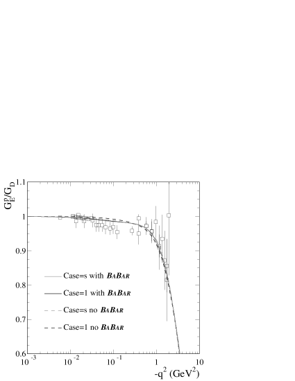
Figure 5: Space-like electric proton EMFF normalized to the dipole, in case=1 and case=$s$, including and not the BABAR data.

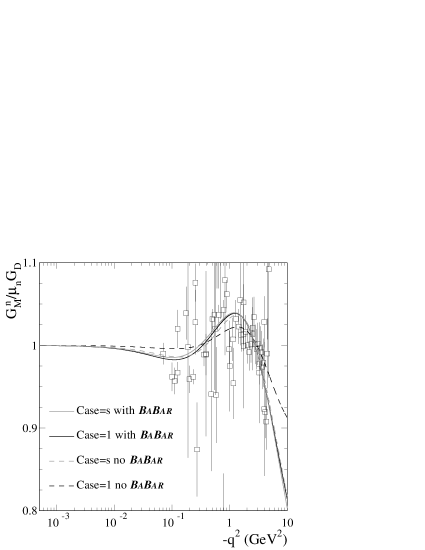
Figure 6: Space-like magnetic neutron EMFF normalized to the dipole and $\mu_{n}$, in case=1 and case=$s$, including and not the BABAR data.

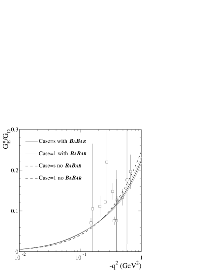
Figure 7: Space-like electric neutron EMFF normalized to the dipole, in case=1 and case=$s$, including and not the BABAR data.

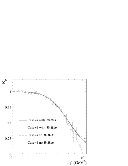
Figure 8: Space-like ratio $R_{p}=\mu_{p}\,G_{E}^{p}/G_{M}^{p}$ normalized to $\mu_{p}$, in case=1 and case=$s$, including and not the BABAR data.

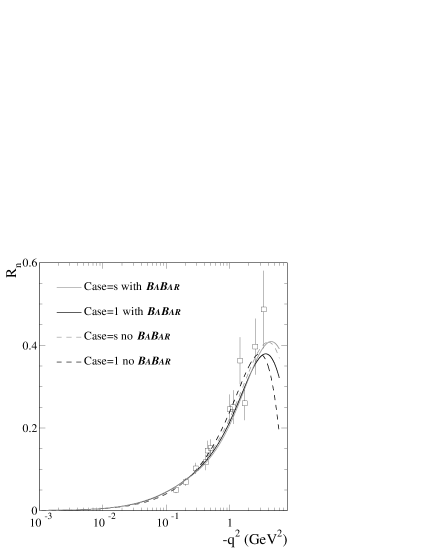
Figure 9: Space-like ratio $R_{n}=\mu_{n}\,G_{E}^{n}/G_{M}^{n}$ normalized to $\mu_{n}$, in case=1 and case=$s$, including and not the BABAR data.

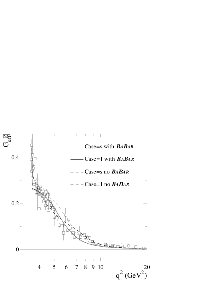
Figure 10: Time-like effective proton FF data (nine sets [13, 14, 15, 16, 17, 18, 19, 20, 21]) and fit, in case=1 and case=$s$, including and not the BABAR data.

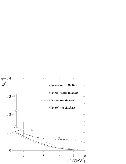
Figure 11: Time-like effective neutron FF data (only FENICE [13]) and fit, in case=1 and case=$s$, including and not the BABAR data.

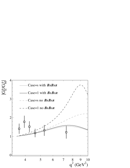
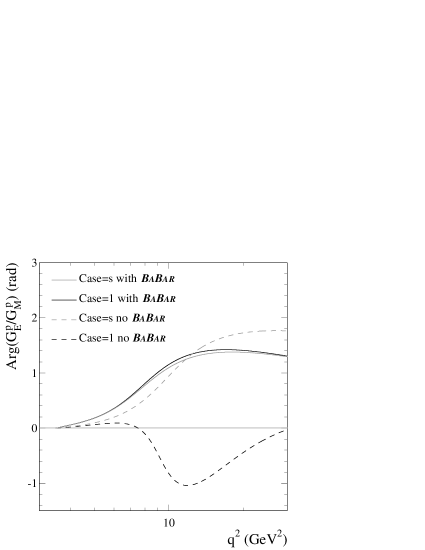
Figure 12: Modulus of the ratio $G_{E}^{p}/G_{M}^{p}$, data [21] and prediction, in the time-like region, in case=1 and case=$s$, including and not the BABAR data.

Figure 13: Prediction for the phase of the ratio $G_{E}^{p}/G_{M}^{p}$, in the time-like region, in case=1 and case=$s$, including and not the BABAR data.

7 Discussion

The Lomon-Gari-Krumpelman Model [5] was developed for and fitted to space-like EMFF data. To enable the model to include the time-like region only the vector meson (of non-negligible width) propagators needed revision to appropriately represent a relativistic BW form at their pole in the time-like region. Two such forms are discussed above, case=1, the minimal alteration from the non-relativistic BW form, and case=$s$ derived from relativistic perturbation theory. The resulting modification in the space-like region is minor and affected the fit there very little.
With the new form of the vector meson propagators the simultaneous fit to the space-like EMFF and the time-like nucleon-pair production data was satisfactory as seen in Figs. 5-11 and by the $\chi^{2}$ values of Table 3.
The $\chi^{2}$ contributions from each space-like EMFF differ little between case=1 and case=$s$ and are approximately the same as in the space-like only fit of Ref. [12].
However the fit in the time-like region, as measured by $\chi^{2}$, is qualitatively poorer when the BABAR data [21] are included ($\chi^{2}$/d.o.f.=2.5) than when that set of data is omitted ($\chi^{2}$/d.o.f.=0.5 for case=1, and is 1.0 for case=$s$). As the quality of the fit is poorer when the BABAR data are included it may indicate an inadequacy in the model. However the energy of the nucleon pairs produced in the BABAR experiment, unlike that of the exclusive pair production [13]-[20], depends on the assumption that the observed photon is from electron or positron emission and is not accompanied by a significant amount of other radiation. The resultant theoretical error is not fully known although relevant calculations have been made [22]. The angular distributions may be sensitive to these radiation effects affecting the values of the $|G_{E}^{p}/G_{M}^{p}|$ ratio whose data are displayed in Fig. 13 together with our prediction.
Figures 5-9 are extended to higher momentum-transfers than the present data to show how the four different fits may be discriminated by new data. Figure 9 for $R_{p}$ indicates that at the higher momentum-transfers extended data may discriminate the smaller case=$s$ no BABAR  prediction from the larger case=1 and case=$s$ with-BABAR predictions and from the still larger case=1 no-BABAR prediction. Figure 9 for $R_{n}$ shows that at high momentum-transfer the case=$s$ predictions are higher than those for case=1.
Figure 11 is extended in energy for the same reason. It clearly shows that at higher energy case=1 no-BABAR  may be discriminated from the other three fits by moderately precise data.
An extension of Fig. 11 would only show the production of proton pairs remaining very close to zero. However in the range of energy already covered it is evident that the case=$s$ no-BABAR result is difficult to reconcile with the BABAR data for $s=5-7$ GeV². However for $s=7.5-8.5$ GeV² the no-BABAR fits are closer to the BABAR data than are the with-BABAR fits.
Figures 13 and 13 show that experiments in the time-like region for the ratio $|G_{E}^{p}/G_{M}^{p}|$ and the phase difference of $G_{E}^{p}$ and $G_{M}^{p}$ would be effective in discriminating between the models presented here and other models as well.

Appendix A:
Dispersion Relations

Dispersion relations are based on the Cauchy theorem. Consider a function $F(z)$, analytic in the whole $z$ complex plane with the discontinuity cut $(s_{0},\infty)$. If that function vanishes faster than $1/\ln|z|$ as $|z|$ diverges we can write the spectral representation

$$F(z)=\frac{1}{\pi}\int_{s_{0}}^{\infty}\frac{\mbox{Im}[F(x)]dx}{x-z}\,.$$ (A.1)

This is the so-called DR for the imaginary part where it is understood that the imaginary part is taken over the upper edge of the cut.
The extension to the case where there is a finite number of additional isolated poles is quite natural. Indeed, considering a function with the set of $N$ poles $\{z_{j}\}$ ($j=1,\ldots,N$) of Sec. 4.1, under the same conditions we obtain the spectral representation

$$F(z)+2\pi i\sum_{j=1}^{N}{\rm Res}\left[\frac{F(z^{\prime})}{z^{\prime}-z},z_{j}\right]=\frac{1}{\pi}\int_{s_{0}}^{\infty}\frac{\mbox{Im}[F(x)]dx}{x-z}\,,$$ (A.2)

where Res$\big{[}g(z),z_{0}\big{]}$ stands for the residue of the function $g(z)$ at $z=z_{0}$. Furthermore, since we know the poles, we can use the more explicit form

$$F(z)=\frac{f(z)}{\prod_{j=1}^{N}(z-z_{j})}\,,$$

where $f(z)$ is the pole-free part of $F(z)$, but it has the same discontinuity cut. Using this form in the residue definition of eq. (A.2) and defining $\widetilde{F}(z)$ as the regularized version of $F(z)$, we have

$$\widetilde{F}(z)=F(z)+\sum_{k=1}^{N}\frac{f(z_{k})}{\prod_{k=1,k\not=j}^{N}(z_{k}-z_{j})}\frac{1}{z_{k}-z}=\frac{1}{\pi}\int_{s_{0}}^{\infty}\frac{\mbox{Im}[F(x)]dx}{x-z}\,$$

which is exactly the same expression as eq. (36). In other words, the DR procedure, using only the imaginary part of a generic function, which is suffering or not from the presence of unwanted poles, guaranties regularized analytic continuations, the poles, even if unknown, are automatically subtracted.

Appendix B:
A third case

We consider a regularized vector meson propagator [23]

$$D(s)=\frac{1}{M_{0}^{2}-s+\Pi(s)}\,,$$

where $M_{0}$ is the bare mass of the meson and $\Pi(s)$ is the scalar part of the tensor correlator. The imaginary part, due to the pion loop, can be obtained using the so-called Cutkosky rule [24] as

$$\mbox{Im}\,\Pi(s)=-\gamma_{0}\,\sqrt{\frac{(s-\tilde{s}_{0})^{3}}{s}}\,\theta(s-\tilde{s}_{0})\,,\hskip 28.45274pt\gamma_{0}=\frac{\Gamma_{0}M^{2}}{\sqrt{(M^{2}-\tilde{s}_{0})^{3}}}\,.$$ (B.1)

The real part of $\Pi(s)$ represents the correction to the bare mass $M_{0}$ in such a way that the dressed mass becomes

$$M^{2}=M_{0}^{2}+\mbox{Re}\,\Pi(s)\,.$$

It follows that the propagator can be written in terms of $M^{2}$ and the only imaginary part of $\Pi(s)$

$$D(s)=\frac{1}{M^{2}-s-i\,\mbox{Im}\,\Pi(s)}=\frac{1}{M^{2}-s-i\,\theta(s-\tilde{s}_{0})\,\gamma_{0}\,\sqrt{(s-\tilde{s}_{0})^{3}/s}}\,.$$ (B.2)

Actually, only the imaginary part of this expression makes sense because of the Heaviside step function in the definition of eq. (B.1), nevertheless, using DR, one can determine the complete propagator starting just from its imaginary part. The propagator is expected to be real below the threshold $\tilde{s}_{0}$. In particular, using eq. (A.1) for $t<\tilde{s}_{0}$, we have

$$D(t)=\frac{1}{\pi}\int_{\tilde{s}_{0}}^{\infty}\frac{\mbox{Im}\,D(s)ds}{s-t}=\frac{\gamma_{0}}{\pi}\int_{\tilde{s}_{0}}^{\infty}\frac{\sqrt{s(s-\tilde{s}_{0})^{3}}\,ds}{[s(M^{2}-s)^{2}+\gamma_{0}^{2}(s-\tilde{s}_{0})^{3}](s-t)}\,,$$ (B.3)

while the real part over the time-like cut $(\tilde{s}_{0},\infty)$, i.e. for $s>\tilde{s}_{0}$, is

$$\mbox{Re}\,D(s)=\frac{1}{\pi}\Pr\!\!\int_{\tilde{s}_{0}}^{\infty}\frac{\mbox{Im}\,D(s^{\prime})ds^{\prime}}{s^{\prime}\!-\!s}=\frac{\gamma_{0}}{\pi}\Pr\!\!\int_{\tilde{s}_{0}}^{\infty}\frac{\sqrt{s^{\prime}(s^{\prime}\!-\!\tilde{s}_{0})^{3}}\,ds^{\prime}}{[s^{\prime}(M^{2}\!-\!s^{\prime})^{2}\!+\!\gamma_{0}^{2}(s^{\prime}\!-\!\tilde{s}_{0})^{3}](s^{\prime}\!-\!s)}\,.$$ (B.4)

In this case the “natural” space-like extension of the original form given in eq. (B.2) is no more possible, in fact such a form, when we forget the Heaviside function in the denominator, develops a second cut which extends over the whole space-like region. It follows that we can not write an expression like

$$\mathbb{R}\ni\widetilde{D}(s<\tilde{s}_{0})\not=\frac{1}{M^{2}-s-i\,\sqrt{(s-\tilde{s}_{0})^{3}/s}}\,-\underbrace{\sum_{k}\frac{R_{k}}{s-s_{k}}}_{\mbox{Physical poles}}\,,$$

where we get, in the space-like region, a regular and real propagator simply by subtracting the physical poles.
The only possibility to go below threshold is to use the DR’s of eq. (B.3) and (B.4). We compute explicitly the DR integrals using the substitution

$$x=\sqrt{1-\frac{\tilde{s}_{0}}{s}}\hskip 14.22636pt\Longrightarrow\hskip 14.22636pt\left\{\begin{array}[]{l}\displaystyle s=\frac{\tilde{s}_{0}}{1-x^{2}}\\ \\ \displaystyle ds=2\tilde{s}_{0}\frac{x\,dx}{(1-x^{2})^{2}}\\ \\ \displaystyle s\in(\tilde{s}_{0},\infty)\to x\in(0,1)\\ \end{array}\right.\,.$$ (B.10)

The regularized form for $D(s)$ is

$$\widetilde{D}(s)=\!\left\{\!\!\begin{array}[]{ll}\displaystyle\frac{-1}{\pi\,s\,\gamma_{0}}\sum_{i=0}^{3}\frac{\xi_{i}^{3}\ln\left(\frac{\xi_{i}+1}{\xi_{i}-1}\right)}{\prod_{k\not=i}^{3}(x_{i}^{2}-x_{k}^{2})}&\hskip 11.38109pts\leq\tilde{s}_{0}\\ &\\ \displaystyle-\frac{{\displaystyle\sum_{i=1}^{3}}\frac{\xi_{i}^{3}\ln\left(\frac{\xi_{i}+1}{\xi_{i}-1}\right)}{\prod_{k\not=i}^{3}(x_{i}^{2}-x_{k}^{2})}+\frac{x_{0}^{3}\ln\left|\frac{\xi_{0}+1}{\xi_{0}-1}\right|}{\prod_{k\not=0}^{3}(x_{0}^{2}-x_{k}^{2})}}{\pi\,s\,\gamma_{0}}\!+\!\displaystyle\frac{i\,\gamma_{0}\sqrt{s(s\!-\!\tilde{s}_{0})^{3}}}{s(M^{2}\!-\!s)^{2}\!+\!\gamma_{0}^{2}(s\!-\!\tilde{s}_{0})^{3}}&\hskip 11.38109pts>s_{0}\\ \end{array}\right.\!\!\!\!.$$ (B.14)

The four values $x_{i}^{2}$ ($i=0,1,2,3$), with $\xi_{i}\equiv\sqrt{x_{i}^{2}}$, are the roots of the 4^th-degree polynomial in $x^{2}$, which represents the denominator of the integrands in both DR’s:

$$\left\{\left[\left(1-x^{2}\right)M^{2}/\tilde{s}_{0}-1\right]^{2}/\gamma_{0}^{2}+x^{6}\right\}\left(\tilde{s}_{0}/t-1+x^{2}\right)\,,$$ (B.15)

in particular: $x_{0}^{2}=1-\tilde{s}_{0}/s$, is the only root that depends on $s$, while the three $x_{i}$, with $i=1,2,3$, are the constant zeros of the first polynomial factor of two in eq. (B.15). The value at $s=0$ can be obtained as

$$\widetilde{D}(0) = -\frac{1}{\pi\,s_{0}\,\gamma_{0}}\sum_{i=1}^{3}\frac{x_{i}^{3}\ln\left(\frac{x_{i}+1}{x_{i}-1}\right)}{\mathop{\prod_{k\not=i}^{3}}_{k=1}(x_{i}^{2}-x_{k}^{2})}\,.$$

Concerning the asymptotic behavior, when $s\to\pm\infty$, i.e.: $x_{0}^{2}\to 1$, is

$$\widetilde{D}(s)\mathop{\sim}_{|s|\to\infty}\frac{1}{\pi\gamma_{0}\prod_{i=1}^{3}(1-x_{i}^{2})}\,\frac{\ln|s|}{s}=\frac{\gamma_{0}}{\pi(1+\gamma_{0}^{2})}\,\frac{\ln|s|}{s}\,,$$

where the last identity follows because the product at denominator is just the $3^{\rm th}$ degree $x^{2}$-polynomial of eq. (B.15) evaluated at $x^{2}=1$.
A data fit was not made for this case because the resonance shape it produces is intermediate between the fitted case=1 and case=$s$.

Appendix C:
The threshold behavior

The effective proton and neutron EMFF’s extracted from the cross section data through the formula of eq. (77) have a quite steep enhancement towards the threshold, i.e. when $q^{2}\to(2M_{N})^{2}$. This is a consequence of the almost flat cross section measured in the near-threshold region: $(2M_{N})^{2}\leq q^{2}\leq(2\,{\rm GeV})^{2}$. Such a flat behavior is in contrast with the expectation in case of a smooth effective FF, which gives, near threshold, a cross section proportional to the velocity of the outgoing nucleon $\sqrt{1-4M_{N}^{2}/q^{2}}$. Moreover, in the threshold region the formula of eq. (77) has to be corrected to account for $N\overline{N}$ finale state interaction. In particular, in the Born cross section formula, in case of proton-antiproton, we have to consider the correction due to their electromagnetic attractive interaction [25]. Such a correction, having a very weak dependence on the fermion pair total spin, factorizes and, in case of pointlike fermions, corresponds to the squared value of the Coulomb scattering wave function at the origin, it is also called Sommerfeld-Schwinger-Sakharov rescattering formula [26]. Besides the Coulomb force also strong interaction could be considered. Indeed, when final hadrons are produced almost at rest they interact strongly with each other before getting outside the range of their mutual forces [27]. Indeed there is evidence for near threshold quasi-bound $N\overline{N}$  states with widths in the tens of MeV [28]. It follows that EMFF values in this energy region are affected by different kinds of corrections whose form and interplay are not well known. Hence we decided to include in the present analysis only data above $q^{2}=4\,{\rm GeV}^{2}$, to avoid the threshold region.
Figures 15 and 15 show the residue data-over-fit for the proton and neutron effective FF’s, respectively. They have been obtained dividing the fit functions shown in Figs. 11 and 11 by the corresponding data on $|G_{\rm eff}^{p,n}|$. The threshold enhancement of the proton data exceeds the fit by a factor of more then two and, in the neutron case, even within large errors, the factor is about three.

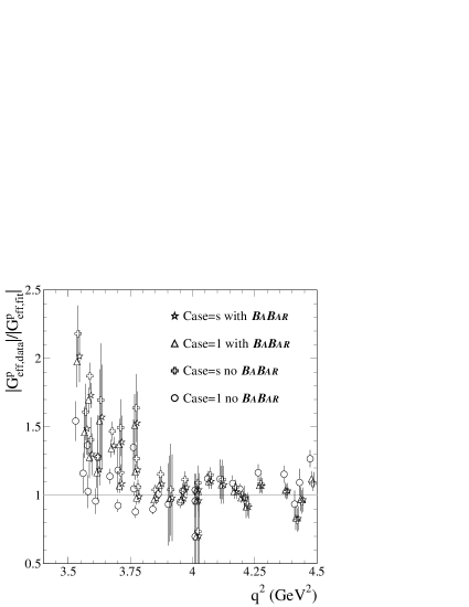
Figure 14: Residue for the proton effective FF: $|G_{\rm eff,\,data}^{p}|/|G_{\rm eff,\,fit}^{p}|$, where $|G_{\rm eff,\,fit}^{p}|$ has been obtained considering only data with $q^{2}\geq 4\,{\rm GeV}^{2}$.

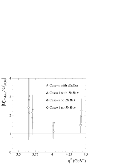
Figure 15: ​Residue for the neutron effective FF: $|G_{\rm eff,\,data}^{n}|/|G_{\rm eff,\,fit}^{n}|$, where $|G_{\rm eff,\,fit}^{n}|$ has been obtained considering only data with $q^{2}\geq 4\,{\rm GeV}^{2}$.

References

- [1] C. F. Perdrisat, V. Punjabi and M. Vanderhaeghen, Prog. Part. Nucl. Phys. 59, 694 (2007) [arXiv:hep-ph/0612014].
- [2] F. Iachello, A. D. Jackson and A. Lande, Phys. Lett. B 43, 191 (1973).
- [3] M. F. Gari and W. Krüempelmann, Phys. Lett. B 274, 159 (1992) [Erratum-ibid. B 282, 483 (1992)].
- [4] See e.g. E. Tomasi-Gustafsson, F. Lacroix, C. Duterte and G. I. Gakh, Eur. Phys. J. A 24, 419 (2005) [arXiv:nucl-th/0503001].
-
[5]
E. L. Lomon,
arXiv:nucl-th/0609020;
E. L. Lomon, Phys. Rev. C 66, 045501 (2002) [arXiv:nucl-th/0203081];
E. L. Lomon, Prepared for 9th International Conference on the Structure of Baryons (Baryons 2002), Newport News, Virginia, 3-8 March 2002;
E. L. Lomon, Phys. Rev. C 64, 035204 (2001) [arXiv:nucl-th/0104039]. - [6] L. L. Foldy, Phys. Rev. 87, 688 (1952).
- [7] L. N. Hand, D. G. Miller and R. Wilson, Rev. Mod. Phys. 35, 335 (1963).
- [8] P. Mergell, U. G. Meissner and D. Drechsel, Nucl. Phys. A 596, 367 (1996) [arXiv:hep-ph/9506375].
-
[9]
S. J. Brodsky and G. R. Farrar,
Phys. Rev. Lett. 31, 1153 (1973);
V. Matveev et al., Nuovo Cimento Lett. 7 (1973) 719;
G. P. Lepage and S. J. Brodsky, Phys. Rev. D 22, 2157 (1980). -
[10]
R. J. Eden, P. V. Landshoff, D. I. Olive, and J. C. Polkinghorne,
The Analytic S-matrix (Cambridge University Press, Cambridge, England, 1966);
G. F. Chew, The Analytic S-Matrix (Benjamin, New York, 1966). - [11] K. Nakamura et al. (Particle Data Group), J. Phys. G 37, 075021 (2010).
- [12] C. Crawford et al., Phys. Rev. C 82, 045211 (2010) [arXiv:1003.0903 [nucl-th]].
- [13] A. Antonelli et al. [FENICE Collaboration], Nucl. Phys. B 517, 3 (1998).
- [14] B. Delcourt et al. [DM1 Collaboration], Phys. Lett. B 86, 395 (1979).
- [15] D. Bisello et al. [DM2 Collaboration], Nucl. Phys. B 224, 379 (1983).
- [16] M. Ablikim et al. [BES Collaboration], Phys. Lett. B 630, 14 (2005) [arXiv:hep-ex/0506059].
- [17] T. K. Pedlar et al. [CLEO Collaboration], Phys. Rev. Lett. 95, 261803 (2005) [arXiv:hep-ex/0510005].
- [18] G. Bardin et al. [LEAR Collaboration], Nucl. Phys. B 411 (1994) 3.
- [19] T. A. Armstrong et al. [E760 Collaboration], Phys. Rev. Lett. 70, 1212 (1993).
- [20] M. Ambrogiani et al. [E835 Collaboration], Phys. Rev. D 60, 032002 (1999).
- [21] B. Aubert et al. [BABAR Collaboration], Phys. Rev. D 73, 012005 (2006) [arXiv:hep-ex/0512023].
- [22] V. V. Bytev, E. A. Kuraev, E. Tomasi-Gustafsson and S. Pacetti, Phys. Rev. D 84, 017301 (2011) [arXiv:1103.4470 [hep-ph]].
- [23] F. Klingl, N. Kaiser and W. Weise, Z. Phys. A 356, 193 (1996) [arXiv:hep-ph/9607431].
- [24] C. Itzykson and J.-B. Zuber, Quantum Field Theory, Mc Graw-Hill, New York (1980).
- [25] R. Baldini, S. Pacetti, A. Zallo and A. Zichichi, Eur. Phys. J. A 39, 315 (2009) [arXiv:0711.1725 [hep-ph]].
-
[26]
A. D Sakharov, Zh. Eksp. Teor. Fiz. 18, 631 (1948)
[Sov. Phys. Usp. 34, 375 (1991)];
A. Sommerfeld, Atombau und Spektralliniem (Vieweg, Braunschweig, 1944), Vol. 2, p.130;
J. Schwinger, Particles, Sources, and Fields, Vol. III, p. 80. - [27] J. Haidenbauer, H. W. Hammer, U. G. Meissner and A. Sibirtsev, Phys. Lett. B 643, 29 (2006) [arXiv:hep-ph/0606064].
- [28] S. Wycech and B. Loiseau, arXiv-hep-ph/0508064v1(2005).